A Novel Hybrid Model Combining the Support Vector Machine (SVM) and Boosted Regression Trees (BRT) Technique in Predicting PM₁₀ Concentration

Abstract

The PM₁₀ concentration is subject to significant changes brought on by both gaseous and meteorological variables. The aim of this research was to explore the performance of a hybrid model combining the support vector machine (SVM) and the boosted regression trees (BRT) technique in predicting the PM₁₀ concentration for 3 consecutive days. The BRT model was trained by utilizing maximum daily data in the cities of Alor Setar, Klang, and Kuching from the years 2002 to 2017. The SVM–BRT model can optimize the number of predictors and predict PM₁₀ concentration; it was shown to be capable of predicting air pollution based on the models’ performance with NAE (0.15–0.33), RMSE (10.46–32.60), R² (0.33–0.70), IA (0.59–0.91), and PA (0.50–0.84). This was accomplished while saving training time by reducing the feature size given in the data representation and preventing learning from noise (overfitting) to improve accuracy. This knowledge establishes the foundation for the development of efficient methods to prevent and/or minimize the health effects of PM₁₀ exposure on one’s health.

1. Introduction

The Malaysian Department of Environment (DoE) maintains a continuous monitoring system for the country’s ambient air quality, which is currently set at 68. The calculation of the Air Pollution Index (API) uses the concentration of six major pollutants: particulate matter 10 μm or less (PM₁₀), particulate matter 2.5 μm or less (PM_2.5), ground-level ozone (O₃), carbon monoxide (CO), nitrogen dioxide (NO₂), and sulfur dioxide (SO₂). Up until 2017, PM₁₀ was the primary contributor to Malaysia’s API; however, from the middle of 2017, PM_2.5 had a considerable influence on the API [1]. Furthermore, according to one study [2], particulate matter (PM₁₀ and PM_2.5) is one of the most significant pollutants with the potential to impact human health. Therefore, the primary emphasis of this study will be on predicting the PM₁₀ concentration, given that PM_2.5 was not completely tracked until 2018.

In recent years, there has been a growing interest in a variety of models to predict levels of air pollution. Artificial neural networks (ANNs) are the technique most frequently employed to generate forecasts of the PM₁₀ concentration [3,4,5]. However, according to one study [6], a validation of the ANN model’s predictive component deemed it insufficient to determine whether it is capable of accurately capturing the underlying dynamics between independent and dependent variables. Furthermore, the random forest (RF) method showed subpar model accuracy in machine learning decision trees during the Southern Italian summer [7].

The BRT was used to estimate NO_x concentrations at roadside locations and discover correlations between background levels, traffic density, and meteorological conditions [8]. On the other hand, BRT has also been employed to estimate particle number count concentrations (PNC) and coarse particles in a coastal region of Malaysia [9]. The results revealed that the BRT model provided the best fit for a diverse blend of data types. Furthermore, simulation data that was used in the development of the algorithm model for BRT [10] is the best guideline, particularly in the field of air pollution. A previous study developed a valid dataset to investigate the effects of air pollution on human health and demonstrated that the BRT technique can increase the accuracy of satellite PM_2.5 predictions [11]. These studies only used 5- and 10-fold cross validation (CV) to optimize the number of trees in the BRT, which is one of three strategies was used to optimize the number of trees in BRT, namely, an independent test set (TEST), out-of-bag estimation (OOB), and v-fold cross validation (CV). Therefore, to determine which of the three approaches (CV, OOB, and TEST) is better, this study will compare them and utilize the best approach for optimizing the number of trees in the BRT technique.

The BRT algorithms are sensitive to parameter settings, which means that adjusting the parameters takes a significant amount of time. The large number of additional predictors offered by the algorithms makes the models more complicated, hence they are challenging to interpret and construct [12]. As a result, the feature selection method, which is one of the most crucial components in machine learning [13], is employed to shorten training and usage times. Besides, it helps improve accuracy in a variety of machine learning problems [14]. As stated previously [15], feature selection not only saves training time by reducing the feature size specified in the data representation, it also prevents learning from noise (over fitting) to enhance accuracy. There are three feature selection methods: wrapper, filter, and embedding methods [16]. The filter methods are faster than the wrapper methods and provide higher generalization since they operate independently of the induction procedure [17]. In contrast, embedding methods have a smaller computational overhead than wrapper methods [18]. Hence, this study employed the Support Vector Machine (SVM) weight as a filter approach for feature selection.

Since single BRT models have limited performance, there is potential for hybrid models that integrate BRT with other methods to be more efficient in predicting air pollution. Hybrid prediction models are being created and used more frequently these days, especially for the purpose of forecasting air pollutants. For instance, it was discovered that combining principal components analysis (PCA) with multiple linear regression (MLR) along with feed forward back propagation (FFBP) improved MLR and FFBP models [19]. In another study [20], artificial neural networks (ANN) were combined with principal components analysis (PCA), ANN with Lasso regression, and ANN with elastic-net regression; the hybrid models improved the performance of the MLR and FFBP models. In addition, a novel hybrid model that combines BRT with regularized regression (RR) has also been developed [12]; the findings show that hybrid models perform better than BRT models alone. In conclusion, previous research has shown that hybrid models perform better than single models, demonstrating that hybrid models are able to make better predictions than single models.

The aim of this study was to develop an air pollution model using SVM weight as a feature selection combined with the BRT technique. According to the available research, a study that makes use of such a strategy to forecast the PM₁₀ concentration has never been carried out. The results of the suggested methodology are compared to the predictions made by previous studies.

2. Materials and Methods

2.1. Data Acquisition

Within the scope of this research, secondary monitoring data was analyzed to ascertain and validate the predictive ability for the PM₁₀ concentration. The data were recorded hourly, and their dependability was ensured by the DoE Malaysia’s quality assurance and quality control processes.

Table 1. Selected air monitoring stations.

Location	Latitude	Longitude	Station ID
Islamic Religious Secondary School, Mergong, Alor Setar, Kedah	06°08.218′ N	100°20.880′ E	CA0040
Raja Zarina Secondary School, Klang, Selangor	03°00.620′ N	101°24.484′ E	CA0011
Medical Store, Kuching, Sarawak	01°33.734′ N	110°23.329′ E	CA0004

show the map where the three monitoring stations are located. These stations can be classified as either urban (such as Klang and Alor Setar) or industrial (Kuching). While Klang is located in the west coast region of Peninsular Malaysia, Alor Setar is located in the northern region of Peninsular Malaysia, and Kuching is located in Sarawak, which is in the northwest corner of Borneo Island. The period covered by the data for the three monitoring sites was from 2002 to 2017, and the monitoring records were also converted into maximum daily data.

2.2. Feature Description

Gases such as nitrogen dioxide (NO₂), carbon monoxide (CO), sulfur dioxide (SO₂), particulate matter with an aerodynamic diameter of less than or equal to 10 µm (PM₁₀), and ground-level ozone (O₃); and meteorological parameters such as ambient temperature (T), relative humidity (RH), and wind speed (WS) were the features used in this study. These features were the independent variables (IV) used to predict the PM₁₀ concentration for the next day (D+1), next 2 days (D+2), and the next 3 days (D+3).

Table 2. The selected features for predicting PM₁₀ concentration.

Feature	Role	Unit	Measurements Level
NO2,D	independent variable	ppb	Continuous
COD	independent variable	ppb	Continuous
SO2,D	independent variable	ppb	Continuous
PM10,D	independent variable	µg/m3	Continuous
O3,D	independent variable	ppb	Continuous
TD	independent variable	°C	Continuous
RHD	independent variable	%	Continuous
WSD	independent variable	km/hour	Continuous
PM10,D+1	dependent variable	µg/m3	Continuous
PM10,D+2	dependent variable	µg/m3	Continuous
PM10,D+3	dependent variable	µg/m3	Continuous

describes the features’ role, unit, and their associated measurement level.

2.3. Data Pre-Processing

The maximum daily data were converted from hourly data obtained from Malaysia’s Department of Environment (DoE), Ministry of Environment and Water, between 1 January 2002 and 28 December 2017. The datasets used in this study are protected by confidentiality, but they are accessible to researchers who have signed Data Use Agreements with the Department of Environment (DoE) and Ministry of Environment and Water. A random selection of 80% of the data was used to develop the model, and the remaining 20% was used to validate the model. The analysis was carried out based on the availability of RH monitoring data, as shown in

Table 3. The selected features for predicting PM₁₀ concentration.

Stations	RH Available Date	Total Data Sets	Stations
Alor Setar	22 October 2002–28 December 2017	5548	Alor Setar
Klang	1 October 2002–28 December 2017	5569	Klang
Kuching	3 December 2002–28 December 2017	5505	Kuching

.

The aim of this study was to predict the PM₁₀ concentration 3 days ahead. Under the National Haze Action Plan, in any area with continuous APIs of over 101 for more than 3 days, the government has the authority to issue a warning status [21]. Hence, it is important to be able to have an early warning for any hazardous environmental status.

Prediction systems that rely on continuous data for most of their components face a significant challenge when there are discontinuities in the data. Insufficient information leads to an incorrect appraisal or interpretation of the observation [22]. Researchers in the field of environmental studies frequently run into the issue of missing data because of unpredictable events such as the malfunctioning of instruments, the need for instrument maintenance or repairs, and calibration [23]. Since statistical analyses rely on complete datasets, missing data needs to be dealt with. In this study, the messy data were cleaned up using a technique called linear interpolation. According to previous studies [24,25], this linear interpolation method estimates the missing data better for the air pollution data. The percentage of missing data was added: missing data in Alor Setar was 5.10%, missing data in Klang was 4.74%, and in Kuching it was 5.83%.

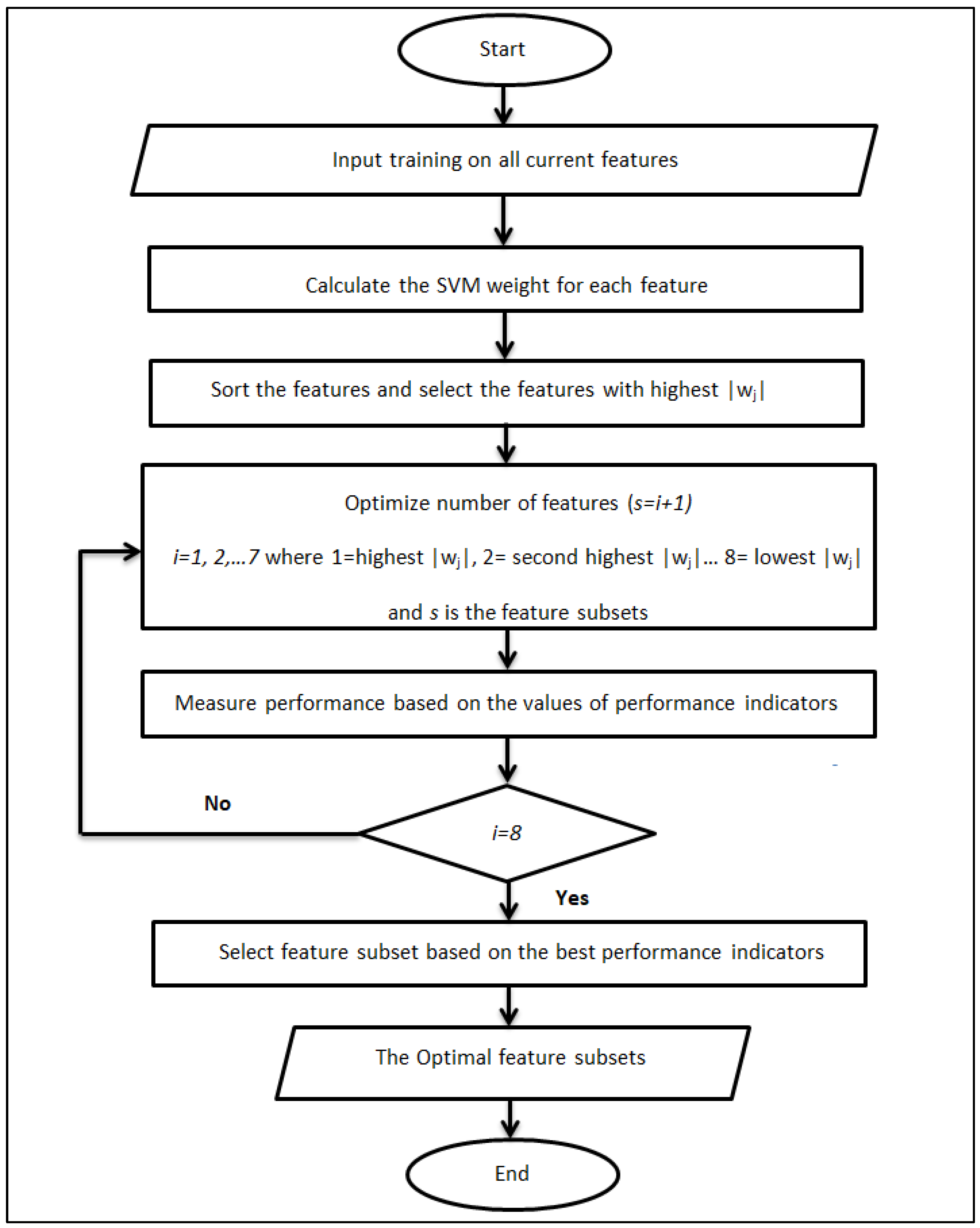
2.4. Feature Selection Using SVM Weight

Classification refers to the development of predictive models for the response variable based on a set of other variables. Feature selection, which utilizes a filter method strategy, is necessary as a pre-processing step before classification. They produce a relevance measure on the training set to exclude the features from the data set that are deemed to be of the least significance. To train a support vector machine (SVM), a weight vector must first be constructed using the training data. Using the weight vector as an indicator, the classifier can decide which features to select.

The SVM classifier works by maximizing the margin to separate the hyperplane (w^Tx + b) between two different groups of data. The threshold that gives the largest margin for making classifications is called the maximal margin classifier. The sample is given by x_i = (x_i1,...,x_md) where m is the number of samples and d is the dimensional feature vector of x_i, which represents the number of distinct features in the model. A class label is given by y_i ∈ {+1, −1} where y_i = 1 for the positive class and y_i = −1 for the negative class. The maximization of the margin corresponds to the following unconstrained optimization problem [16]:

$${\mathbf{w}}^{*}{,\mathrm{b}}^{*},{\xi }^{*}=\arg \underset{\mathbf{w},\mathrm{b},\xi }{\min }\frac{1}{2}{\Vert \mathbf{w}\Vert }^2+\mathrm{C}{\displaystyle \sum _{\mathrm{i}=1}^{\mathrm{m}}{\xi }_{\mathrm{i}}}$$

(1)

$${\mathrm{subject}\mathrm{to}\mathrm{y}}_{\mathrm{i}}({\mathbf{w}}^{\mathrm{T}}{\mathbf{x}}_{\mathrm{i}}+\mathrm{b})\ge {1-\mathsf{\xi }}_{\mathrm{i}}{;\mathsf{\xi }}_{\mathrm{i}}\ge 0;\mathrm{i}=1,\dots ,\mathrm{m}$$

(2)

$\mathbf{w}=\mathrm{m}-\mathrm{dimensional}\mathrm{vector}$

$\mathrm{b}=\mathrm{Scalar}$

${\xi }_{\mathrm{i}}=\mathrm{Penalty}\mathrm{for}$ misclassification or classification with the margin (loss function)

$\mathrm{C}=\mathrm{Penalty}\mathrm{parameter}$ on the training error

In general, the class predictor trained by SVM has the form:

$$\mathrm{prediction}\left(\mathbf{x}\right)=\mathrm{sgn}\left({\mathbf{w}}^{\mathrm{T}}\mathbf{x}+\mathrm{b}\right)=\mathrm{sgn}\left({\displaystyle {\sum }_{\mathrm{j}}{\mathrm{w}}_{\mathrm{j}}{\mathrm{x}}_{\mathrm{j}}+\mathrm{b}}\right)\mathrm{for}\mathbf{w}={\displaystyle {\sum }_{\mathrm{i}}{\mathsf{\alpha }}_{\mathrm{i}}{\mathbf{x}}_{\mathrm{i}}}$$

(3)

where |w_j| is used as the weight of a feature j; features with large |w_j| values have a large influence on the predictions than features with small |w_j| values. Since $\mathbf{w}={\displaystyle {\sum }_{\mathrm{i}}{\mathsf{\alpha }}_{\mathrm{i}}{\mathbf{x}}_{\mathrm{i}}}$ for the linear SVM model, one can regard ||w||² as a function of the training vector x_i, and thus evaluate the influence of feature j on ||w||² by looking at absolute values of partial derivatives of ||w||² with respect to x_ij. For the linear kernel:

$${\displaystyle {\sum }_{\mathrm{i}}\left|\frac{\partial {\Vert \mathbf{w}\Vert }^2}{\partial {\mathrm{x}}_{\mathrm{ij}}}\right|}=\mathrm{k}\left|{\mathrm{w}}_{\mathrm{j}}\right|$$

(4)

where the sum includes the support vectors and k is a constant independent of j. Thus, the features with higher |w_j| values are more influential in determining the width of the margin. Figure 1 shows an illustration of the procedure to obtain the optimum feature subsets.

One predictor was added at a time into the BRT model, starting with the predictor with the highest SVM absolute weight and ending with the predictor with the lowest SVM absolute weight. The process repeats until there are no more predictors to choose from. The overall goal, as proposed previously [26], was to maximize the accuracy of predictions while minimizing the number of predictors.

2.5. BRT Model

Previous studies [27,28,29] provide a comprehensive description of the theoretical foundations of the BRT technique. The BRT tuning parameters include the number of trees (nt) required for optimal prediction; the learning rate (lr), which is the shrinkage parameter used in each iteration to reduce the tree’s contribution; tree complexity (tc), also known as the interaction depth, which is the maximum tree depth of variable interactions; and bag-fraction (bf), which specifies the proportion of data randomly selected to fit each consequent tree.

Therefore, in this study, BRT models with the following parameters were fitted: nt (10,000), lr (0.01), tc (5), and bf (5). These values were suggested in previous studies [9,30] for the purpose of conducting an analysis of the air pollution dataset. Using GBM (version 1.6–3.1) of R programming software (version 3.4.2), the BRT model was fitted from 80% of the data collected to predict the maximum daily PM₁₀ concentration. The general models for this study are listed in Equations (5)–(7). The algorithm used to model BRT is called gradient boosting (GBM) [27].

PM_10,D+1 ~ gbm(PM_10,D,CO_D,NO_2,D,SO_2,D,RH_D,T_D,WS_D,O_3,D

(5)

PM_10,D+2 ~ gbm(P_10,D,CO_D,NO_2,D,SO_2,D,RH_D,T_D,WS_D,O_3,D)

(6)

PM_10,D+3 ~ gbm(PM_10,D,CO_D,NO_2,D,SO_2,D,RH_D,T_D,WS_D,O_3,D)

(7)

PM_10,D+1 = Next day prediction of PM₁₀ concentration

PM_10,D+2 = Next 2 days prediction of PM₁₀ concentration

PM_10,D+3 = Next 3 days prediction of PM₁₀ concentration

PM_10,D = Particulate matter (µg/m³)

CO_D = Carbon monoxides (ppb)

NO_2,D = Nitrogen dioxide (ppb)

SO_2,D = Sulfur dioxide (ppb)

O_3,D = Ozone (ppb)

RH_D = Relative humidity (%)

T_D = Temperature (°C)

WS_D = Wind speed (km/h).

2.6. Hybrid Model

The use of different modelling techniques to improve overall accuracy is referred to as a hybrid model. There are three different types of hybrid models: (a) using one model to generate new variables and then using these new variables in another model; (b) residual fitting, which is a final model that is built repeatedly by transferring results from one methodology to another; and (c) model averaging, which averages two or more predictions [31]. In other words, a hybrid model is a combination of two or more models.

SVM–BRT is a type (a) hybrid model that reduces feature size in the data representation and prevents learning from noise (over-fitting), thereby improving accuracy while cutting down on the amount of time needed for training. A hybrid model that integrates BRT and linear SVM was used to solve the major problem of the BRT technique, namely, the lengthy time taken to adjust the parameters. Figure 2 depicts the procedures involved in obtaining the best predicted model. A novel aspect of this study is the application of hybrid models as a means of enhancing the methodologies that are currently in use.

2.7. Performance Indictor

The models were evaluated based on the model’s error and accuracy using several performance indicators, namely the root mean square error (RMSE), normalized absolute error (NAE), predictive accuracy (PA), agreement index (IA), and coefficient of determination (R²). The model with the best fit is chosen when it has high accuracy (i.e., PA, IA, and R²), which is closer to 1, while the minimal error (i.e., RMSE and NAE) is closer to 0. Equations (8)–(12) show the formulae for the performance indicators used in this study.

$$RMSE=\frac{1}{n-1}{\displaystyle \sum _{i=1}^n{\left(P_i-O_i\right)}^2}$$

(8)

$$NAE=\frac{{\displaystyle \sum _{i=1}^{n}Abs(P_i-O_i)}}{{\displaystyle \sum _{i=1}^n{O}_i}}$$

(9)

$$IA=1-\left[\frac{{\displaystyle \sum _{i=1}^n{\left(P-O_i\right)}^2}}{{\displaystyle \sum _{i=1}^n{\left(\left|P_i-\overline{O}\right|+\left|O_i-\overline{O}\right|\right)}^2}}\right]$$

(10)

$$PA=\frac{{\displaystyle \sum _{i=1}^n{\left(P_i-\overline{O}\right)}^2}}{{\displaystyle \sum _{i=1}^n{\left(O_i-\overline{O}\right)}^2}}$$

(11)

$$R^2={\left(\frac{{\displaystyle \sum _{i=1}^n\left(P_i-\overline{P}\right)\left(O_i-\overline{O}\right)}}{n.S_{pred}.S_{obs}}\right)}^2$$

(12)

where, n = total number of data; P_i = predicted values; $O_i=$ observed values; $\overline{P}=$ mean of predicted values; $\overline{O}=$ mean of observed values.

3. Results and Discussion

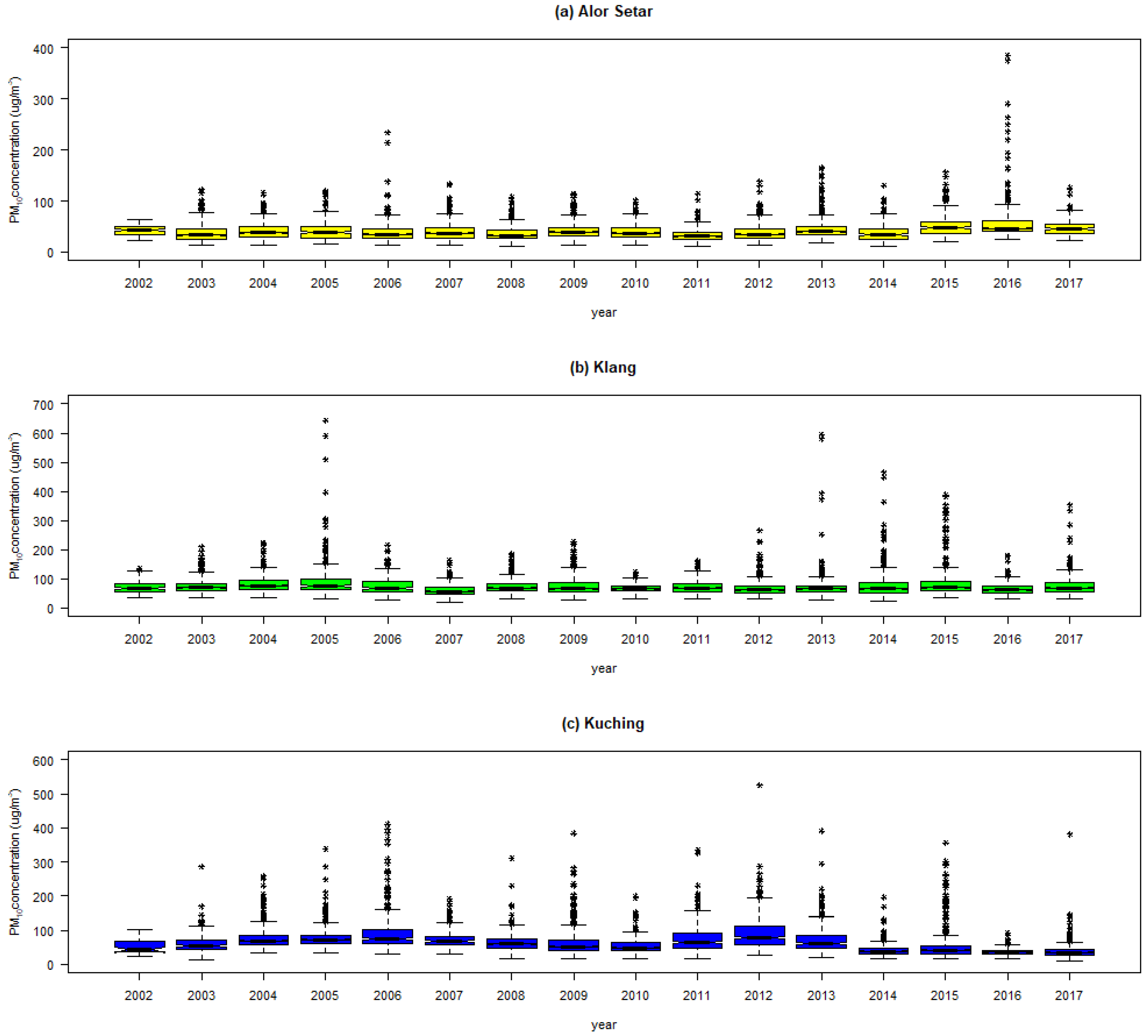
3.1. Descriptive Statistics

Descriptive statistics for the maximum daily data (2002–2017) for Alor Setar, Klang, and Kuching are presented in

Table 4. Summary of the descriptive statistics.

Stations	Parameters (Unit)	Statistical Parameter
		Mean	Median	Standard Deviation	Skewness	Kurtosis	Maximum
Alor Setar	PM10 (μg/m3)	41.99	38	20.84	4.03	40.05	385
	O3 (ppb)	34.27	32	14.86	0.82	1.05	118
	CO (ppb)	560.3	540	246.71	1.71	7.36	3060
	NO2 (ppb)	15.2	14	5.85	1.1	2.97	58
	SO2 (ppb)	1.05	1	0.93	0.99	2.32	8
	RH (%)	89.35	91	8.07	−1.77	3.81	100
	T (°C)	32.42	32.7	2.77	−1.23	3.21	39.5
	WS (Km/h)	10.53	10.7	3.74	0.3	1.78	33.5
Klang	PM10 (μg/m3)	75.05	68	37.78	4.89	44.82	643
	O3 (ppb)	44.74	42	19.33	0.66	0.48	127
	CO (ppb)	1611.43	1440	774.87	2.65	16.04	10500
	NO2 (ppb)	38.34	37	12.67	0.36	0.89	128
	SO2 (ppb)	6.6	5	6.52	8.67	119.11	150
	RH (%)	83.71	84	6.93	−0.71	1.37	100
	T (°C)	33.34	33.6	2.22	−0.74	0.74	38.5
	WS (Km/h)	9.15	9.6	5.02	25.33	1326.95	271
Kuching	PM10 (μg/m3)	65.38	57	39.51	2.99	15.72	526
	O3 (ppb)	23.66	22	9.74	0.78	1.54	82
	CO (ppb)	892.21	780	486.34	1.66	5.28	5080
	NO2 (ppb)	12.64	12	5.85	2.94	40.09	123
	SO2 (ppb)	3.66	3	4.13	7.42	121.54	100
	RH (%)	94.6	95	3.29	−1.03	6.37	100
	T (°C)	33.24	33.21	2.47	−0.38	2.83	53
	WS (Km/h)	11.29	11.3	3.56	5	110.71	99

. The highest mean concentration of PM₁₀ was recorded as 41.99 µg/m³ (Alor Setar), 75.05 µg/m³ (Klang), and 65.38 µg/m³ (Kuching). The established 24-h mean reading for national ambient air quality standards for PM₁₀ concentration was 50 µg/m³ [31,32,33]. Hence, based on the result, Klang and Kuching stations have a high concentration, which is consistent with the findings of previous studies [28,29,30] that indicate a similar pattern of PM₁₀. The reason was because Malaysia experienced a slight haze episode associated with local and transboundary haze from neighboring countries [1].

Additionally, compared to O₃, SO₂, and NO₂, the mean concentration of CO was found to be the highest in all selected locations. According to previous studies [33,34,35], this is due to their location as they are surrounded by numerous industrial, residential, and commercial areas, in addition to the emissions from motor vehicles. High skewness values in Alor Setar (4.03), Klang (4.89), and Kuching (2.99) showed that there were both high particulate events and extreme events that caused PM₁₀ concentrations to rise in all three places.

The box plot in Figure 3 illustrates the PM₁₀ concentrations for the maximum daily readings over the last 16 years at Alor Setar, Klang, and Kuching. Alor Setar had the highest PM₁₀ concentration in 2016, as shown in Figure 3a. The land and forest fires in Central Sumatra, Indonesia, which were brought about by the Southwest Monsoon winds, are said to have had a negative impact on this situation [1]. On 11 August 2005, the air quality in Klang reached an all-time high with a PM₁₀ reading of 643 g/m³. According to a previous study [36], the air quality during that time was hazardous/dangerous due to a dense haze period. This dense haze period was deemed to be the primary factor for the next 10 years of high PM₁₀ values recorded. Lastly, from 2002 to 2017, the highest PM₁₀ concentration in Kuching was reported in October 2012, which was due to emissions from vehicles as well as forest fires that were started for agricultural purposes in Central and Northern Sumatra, Indonesia [35].

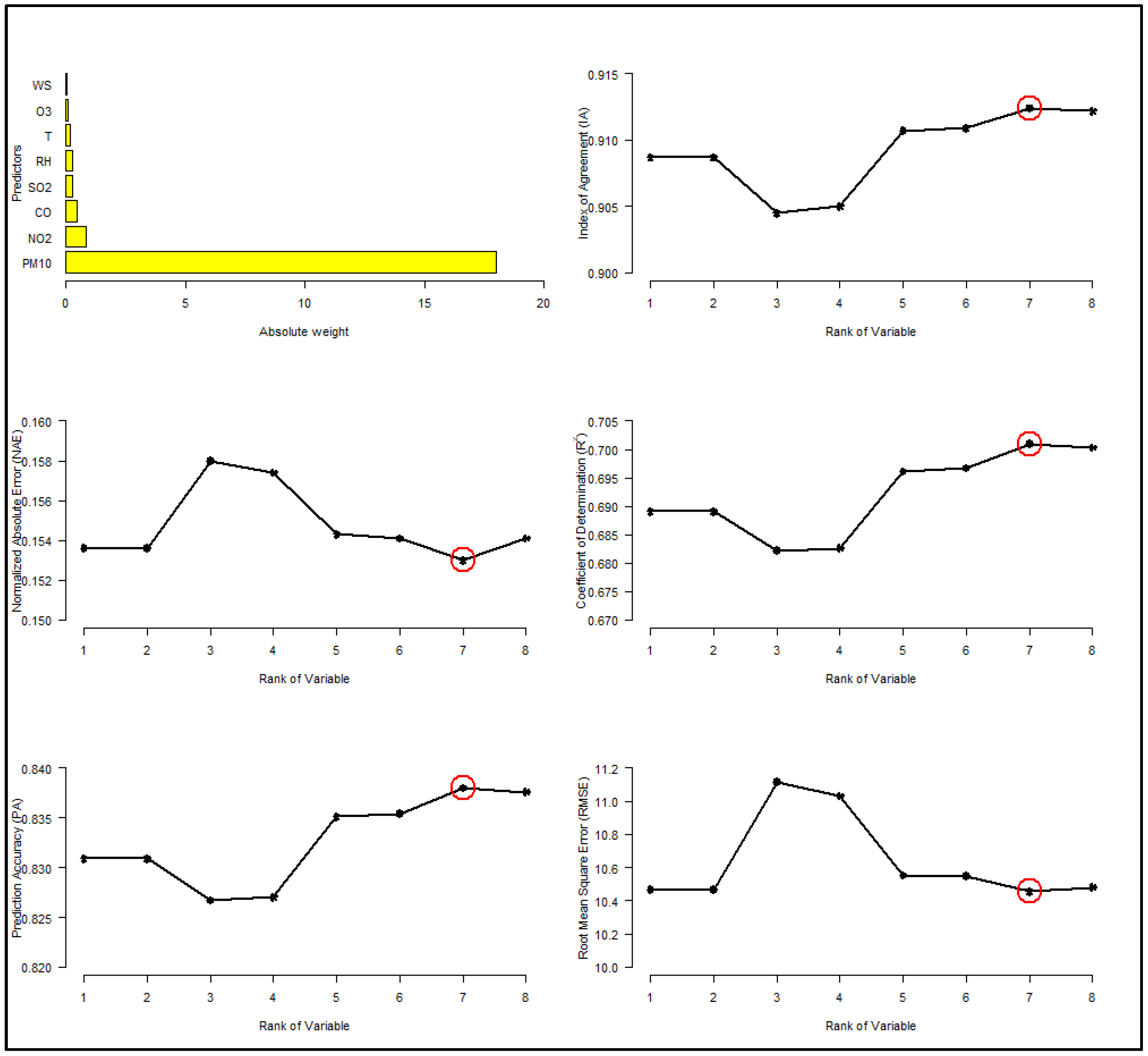
3.2. Optimizing the Number of Predictors (SVM Weight)

The SVM weights were ranked according to their absolute weights; the higher the absolute weight, the more significant the variable was for the purpose of developing a new set of training models. Figure 4, Figure 5 and Figure 6 illustrate the results that occurred when the SVM weight was used as the ranking model, and the red circle showed the best number of variables were selected based on the best performance. Because of the transboundary haze pollution from Sumatra and Kalimantan, Indonesia, the data shows that the PM₁₀ concentration is at the top of the list for all three regions [1].

The BRT model for Alor Setar had the best performance with seven variables were selected and WS was omitted as a predictor: 0.1530 (NAE), 10.4559 (RMSE), 0.9124 (IA), 0.8380 (PA), and 0.7010 (R²) (Figure 4). The results also showed that the Klang station had the best overall performance when six variables were included in the model: 0.1717 (NAE), 21.8568 (RMSE), 0.7829 (IA), 0.8567 (PA), and 0.6118 (R²). However, this performance then rapidly declined (Figure 5); therefore, WS and SO₂ were omitted. The greatest performance (Figure 6) dropped after five variables are chosen for the Kuching station, thus, WS, T, and SO₂ were removed as predictors. Although the highest values of PA and R² indicate that eight variables should be selected, the difference in values (PA and R²) with five variables was too close to be considered significant. As a result, only five variables were determined to be the most accurate predictors of future PM₁₀ concentrations on the following day, the following 2 days, and the following 3 days.

The findings demonstrated that both the type of predictor and the total number of predictors vary depending on location.

Table 5. The selected features for predicting PM₁₀ concentration.

Stations	Selected Predictors
Alor Setar	PM10,D+1 ~ gbm(PM10, NO2, CO, SO2, RH, T, O3) PM10,D+2 ~ gbm(PM10, NO2, CO, SO2, RH, T, O3) PM10,D+3 ~ gbm(PM10, NO2, CO, SO2, RH, T, O3)
Klang	PM10,D+1 ~ gbm(PM10, CO, RH, O3, NO2, T) PM10,D+2 ~ gbm(PM10, CO, RH, O3, NO2, T) PM10,D+3 ~ gbm(PM10, CO, RH, O3, NO2, T)
Kuching	PM10,D+1 ~ gbm(PM10, CO, RH, O3, NO2) PM10,D+2 ~ gbm(PM10, CO, RH, O3, NO2) PM10,D+3 ~ gbm(PM10, CO, RH, O3, NO2)

displays the results that were obtained from the BRT algorithm after using the SVM weight as a feature selection. These results were used to predict the PM₁₀ concentration in Alor Setar, Klang, and Kuching.

3.3. Hybrid Model

In this section, SVM and BRT were combined and the performance level of this hybrid model was investigated.

Table 6. The performance indicators for the SVM–BRT model.

Days	Station	Method	Best Iteration	RMSE	NAE	PA	R2	IA
	Alor Setar	CV	663	10.4559	0.1539	0.8380	0.701	0.9124
		OOB	256	10.0815	0.1527	0.8366	0.6986	0.9113
		TEST	243	10.0011	0.1528	0.8371	0.6994	0.9111
D	Klang	CV	1049	21.9435	0.1725	0.7809	0.6088	0.8644
+		OOB	252	22.3999	0.1754	0.8450	0.5979	0.8450
1		TEST	1094	21.9316	0.1725	0.7812	0.6092	0.8642
	Kuching	CV	931	29.3651	0.2719	0.7032	0.4936	0.8061
		OOB	251	29.8344	0.2800	0.6973	0.4854	0.7725
		TEST	335	29.5637	0.2757	0.7004	0.4897	0.7866
	Alor Setar	CV	347	13.2992	0.222	0.6521	0.4245	0.7909
		OOB	236	13.17	0.2228	0.6491	0.4206	0.7813
		TEST	238	13.169	0.2228	0.6494	0.421	0.7817
D	Klang	CV	245	27.2112	0.2318	0.6176	0.3807	0.7062
+		OOB	227	27.246	0.2321	0.6176	0.3808	0.7
2		TEST	478	27.2512	0.2313	0.6144	0.3768	0.7244
	Kuching	CV	357	34.5616	0.3199	0.6083	0.3694	0.6903
		OOB	244	34.6437	0.3219	0.6111	0.3728	0.675
		TEST	307	34.5745	0.3203	0.6094	0.3706	0.6858
	Alor Setar	CV	475	14.7962	0.2554	0.5357	0.2864	0.6837
		OOB	228	14.76	0.2563	0.5293	0.2796	0.6583
		TEST	345	14.83	0.2562	0.53	0.2805	0.6743
D	Klang	CV	245	31.0173	0.2555	0.5018	0.2514	0.5918
+		OOB	222	31.033	0.2555	0.5017	0.2513	0.5824
3		TEST	859	31.2269	0.2567	0.4967	0.2463	0.619
	Kuching	CV	429	32.6196	0.3259	0.5742	0.3291	0.6844
		OOB	238	32.6295	0.3281	0.5764	0.3316	0.6633
		TEST	250	32.6036	0.3276	0.5768	0.3321	0.6664

displays the results of using the CV, OOB, and TEST methods in the hybrid model to make predictions for the following day (D+1), the following 2 days (D+2), and the following 3 days (D+3). The performance of the BRT model was measured using performance indicators to determine which of the three methods (CV, OOB, and TEST) was the most accurate at predicting the maximum daily concentration of PM₁₀ in Alor Setar, Klang, and Kuching.

According to the findings, CV was the most accurate method for predicting the PM₁₀ concentration for the following day, the following 2 days, and the following 3 days in Alor Setar, Kedah. The PA values ranged from 0.53 to 0.83, the R² values ranged from 0.29 to 0.70, the IA values ranged from 0.68 to 0.91, the NAE values ranged from 0.15 to 0.25, and the RMSE values ranged from 10.46 to 14.79.

Furthermore, the TEST method fits the data better than CV or OOB in predicting the maximum daily PM₁₀ concentration in Klang, Selangor for D+1, whereas CV was the best method for D+2 and D+3. PA values varied between 0.50 and 0.78, R² values between 0.25 and 0.61, IA values between 0.59 and 0.86, NAE values between 0.17 and 0.25, and RMSE values between 21.93 and 31.01.

In the city of Kuching, Sarawak, performance indicators demonstrated that CV was the most effective method for predicting D+1 (RMSE = 29.37, NAE = 0.27, PA = 0.70, R² = 0.49, IA = 0.81) and D+2 (RMSE = 34.56, NAE = 0.32, PA = 0.61, R² = 0.37, IA = 0.71), whereas TEST was the most effective method for predicting D+3 (RMSE = 32.60, NAE = 0.33, PA = 0.58, R² = 0.33, IA = 0.67).

In comparison to the PM_10,D+2 and PM_10,D+3 models, the PM_10,D+1 model had the maximum accuracy of 91% (Alor Setar), 86% (Klang), and 8% (Kuching), with the lowest values of error of 0.15 (Aor Setar), 0.17 (Klang), and 0.27 (Kuching), respectively. In the SVM–BRT model, it was decided that the most effective technique was a combination of the CV and TEST approaches.

In previous studies, several authors have used the BRT technique to predict PM₁₀ concentration. For instance, BRT was used to predict hourly PM₁₀ concentration levels in the City of Makkah [37], with an IA value of 0.66 reported. In addition, a BRT model was used to estimate the PM₁₀ concentration for four different stations [32]; the reported R² varied between 0.61 and 0.72. A hybrid model was developed combining BRT and RR, which was compared with a pure BRT model in predicting the PM₁₀ concentration [12]; for the performance of the pure BRT model, R² = 0.57 RMSE = 14.10, while R² = 0.80 and RMSE = 8.82 for the hybrid model.

Although the previous authors attempted to predict the PM₁₀ concentration, their predicted targets were different from this study. As a result, it is nearly impossible to make direct comparisons with this study. On the other hand, this study’s findings, which were based on performance errors and accuracy, fall within the range that other studies have found.

4. Conclusions

Overall, these results imply that the SVM–BRT model can predict the maximum PM₁₀ concentration that can take place during a given day. The results of the study show that the NAE (0.15–0.33), RMSE (10.46–32.60), R² (0.33–0.70), IA (0.59–0.91), and PA (0.50–0.84) values were good for predicting the next day PM₁₀ concentration. The CV approach was selected as the best method to optimize the number of trees in most of the results, and TEST was also selected as the best method. The results also indicated that the type and number of predictors are different for each location. Seven variables were selected and WS was excluded as a predictor in Alor Setar; six specified variables for the Klang station were used as predicters, with WS and SO₂ excluded; and five variables were chosen for the Kuching station with WS, T, and SO₂ removed as predictors. In conclusion, SVM–BRT is an alternative method for predicting PM₁₀ concentration for the next 3 days at all sites. This model saves training time by reducing the feature size given in the data representation, and prevents learning from noise, also known as overfitting, to improve accuracy. The proposed model can accurately predict maximum daily air pollution episodes within three consecutive days; it can be used as an early warning tool in giving air quality information to local authorities to formulate air quality improvement strategies. However, the proposed model can only be used when the sources and characteristics of PM₁₀ remain the same and can be used in this selected location only.

Here are some propositions for further research concerning the application of BRT models to forecast levels of air pollution. It was found that the CV method in BRT provided the best fit for the data, but it was also discovered that TEST and OOB could be utilized to optimize the number of trees in BRT. In addition to the number of trees, other BRT parameters, such as learning rate and tree complexity, should be investigated to find parameter settings that lead to an alternative solution.

References

1. Department of Environment, Malaysia. Malaysia Environmental Quality Report 2018. Available online: https://enviro2.doe.gov.my/ekmc/wp-content/uploads/2019/09/FULL-FINAL-EQR-30092019.pdf.pdf (accessed on 5 June 2022).
2. Elbayoumi, M.; Ramli, N.A.; Md Yusof, N.F.F.; Yahaya, A.S.; Al Madhoun, W.; Ul-Saufie, A.Z. Multivariate methods for indoor PM10 and PM2.5 modelling in naturally ventilated schools buildings. Atmos. Environ. 2014, 94, 11–21. [Google Scholar] [CrossRef]
3. Perez, P.; Reyes, J. An integrated neural network model for PM10 forecasting. Atmos. Environ. 2006, 40, 2845–2851. [Google Scholar] [CrossRef]
4. Kukkonen, J.; Partanen, L.; Karppinen, A.; Ruuskanen, J.; Junninen, H.; Kolehmainen, M.; Niska, H.; Dorling, S.; Chatterton, T.; Foxall, R.; et al. Extensive Evaluation of Neural Network Models for The Prediction of NO2 and PM10 Concentrations, Compared with a Deterministic Modeling System and Measurements in Central Helsinski. Atmos. Environ. 2003, 37, 4539–4550. [Google Scholar] [CrossRef]
5. Biancofiore, F.; Busilacchio, M.; Verdecchia, M.; Tomassetti, B.; Aruffo, E.; Bianco, S.; Tomasso, S.D.; Colangeli, C.; Rosatelli, G.; Carlo, P.D. Recursive Neural Network Model for Analysis and Forecast of PM10 and PM2.5. Atmos. Pollut. Res. 2017, 8, 652–659. [Google Scholar] [CrossRef]
6. Cabaneros, S.M.; Calautit, J.K.; Hughes, B.R. A review of artificial neural network models for ambient air pollution prediction. Environ. Model. Softw. 2019, 119, 285–304. [Google Scholar] [CrossRef]
7. Stafoggia, M.; Bellander, T.; Bucci, S.; Davoli, M.; de Hoogh, K.; de’ Donato, F.; Gariazzo, C.; Lyapustin, A.; Michelozzi, P.; Renzi, M.; et al. Estimation of daily PM10 and PM2.5 concentrations in Italy, 2013–2015, using a spatiotemporal land-use random-forest model. Environ. Int. 2019, 124, 170–179. [Google Scholar] [CrossRef] [PubMed]
8. Sayegh, A.; Tate, J.E.; Ropkins, K. Understanding how roadside concentrations of NOx are influenced by the background levels, traffic density, and meteorological conditions using Boosted Regression Trees. Atmos. Environ. 2016, 127, 163–175. [Google Scholar] [CrossRef]
9. Yahaya, Z.; Phang, S.M.; Samah, A.A.; Azman, I.N.; Ibrahim, Z.F. The international journal by the Thai Society of Higher Education Institutes on Environment Analysis of Fine and Coarse Particle Number Count Concentrations Using Boosted Regression Tree Technique in Coastal Environment. EnvironmentAsia 2018, 11, 221–234. [Google Scholar]
10. Asri, M.A.M.; Ahmad, S.; Afthanorhan, A. Algorithmic Modelling of Boosted Regression Trees’ on Environment’s Big Data Algorithmic Modelling of Boosted Regression Trees’ on Environment’s Big Data. Elixir Stat. Int. J. 2015, 82, 32419–32424. [Google Scholar]
11. Zhang, T.; He, W.; Zheng, H.; Cui, Y.; Song, H.; Fu, S. Satellite-based ground PM2.5 estimation using a gradient boosting decision tree. Chemosphere 2021, 26, 128801. [Google Scholar] [CrossRef]
12. Ivanov, A.; Gocheva-Ilieva, S.; Stoimenova, M. Hybrid boosted trees and regularized regression for studying ground ozone and PM10 concentrations. AIP Conf. Proc. 2020, 2302, 060005. [Google Scholar]
13. Guyon, I.; Elisseeff, A. An Introduction to Variable and Feature Selection. J. Mach. Learn. Res. 2003, 3, 1157–1182. [Google Scholar]
14. Geng, X.; Liu, T.; Qin, T.; Li, H. Feature Selection for Ranking. In Proceedings of the 30th Annual International ACM SIGIR Conference on Research and Development in Information Retrieval (SIGIR’07), Amsterdam, The Netherlands, 23–27 July 2007; pp. 407–414. [Google Scholar]
15. Mladenic, D.; Brank, J.; Grobelnik, M.; Milic-Frayling, N. Feature selection using linear classifier weights. In Proceedings of the 27th Annual International ACM SIGIR Conference on Research and Development in Information Retrieval, Sheffield, UK, 25–29 July 2004; pp. 234–241. [Google Scholar]
16. Bron, E.E.; Smits, M.; Niessen, W.J.; Klein, S. Feature Selection Based on the SVM Weight Vector for Classification of Dementia. IEEE J. Biomed. Health Inform. 2015, 19, 1617–1626. [Google Scholar] [CrossRef]
17. Sanchez-Marono, N.; Alonso-Betanzos, A.; Tombilla-Sanromán, M. Filter Methods for Feature Selection—A Comparative Study. Intell. Data Eng. Autom. Learn. IDEAL 2007, 4881, 178–187. [Google Scholar]
18. Maldonado, S.; Flores, A.; Verbraken, T.; Baesens, B.; Weber, R. Profit-based feature selection using support vector machines—General framework and an application for customer retention. Appl. Soft Comput. J. 2015, 35, 740–748. [Google Scholar] [CrossRef]
19. Ul-Saufie, A.Z.; Yahaya, A.S.; Ramli, N.A.; Rosaida, N.; Hamid, H.A. Future daily PM10 concentrations prediction by combining regression models and feedforward backpropagation models with principle component analysis (PCA). Atmos. Environ. 2013, 77, 621–630. [Google Scholar] [CrossRef]
20. Suleiman, A.; Tight, M.R.; Quinn, A.D. Hybrid Neural Networks and Boosted Regression Tree Models for Predicting Roadside Particulate Matter. Environ. Model. Assess. 2016, 21, 731–750. [Google Scholar] [CrossRef] [Green Version]
21. Perimula, Y. HAZE: Steps taken to reduce hot spots. New Strait Times 2012. Available online: http://www.nst.com.my/opinion/letters-to-the-editor/haze-steps-taken-to-reduce-hot-spots-1.98115 (accessed on 8 May 2022).
22. Sukatis, F.F.; Mohamed, N.; Zakaria, N.F.; Ul-Saufie, A.Z. Estimation of Missing Values in Air Pollution Dataset by Using Various Imputation Methods. Int. J. Conserv. Sci. 2019, 10, 791–804. [Google Scholar]
23. Noor, N.M.; Yahaya, A.S.; Ramli, N.A.; Abdullah, M.M.A.B. Mean imputation techniques for filling the missing observations in air pollution dataset. Key Eng. Mater. 2014, 594–595, 902–908. [Google Scholar] [CrossRef]
24. Noor, N.M.; Yahaya, A.S.; Ramli, N.A.; Abdullah, M.M.A.B. Filling the Missing Data of Air Pollutant Concentration Using Single Imputation Methods. Appl. Mech. Mater. 2015, 754–755, 923–932. [Google Scholar] [CrossRef]
25. Libasin, Z.; Suhailah, W.; Fauzi, W.M.; ul-Saufie, A.Z.; Idris, N.A.; Mazeni, N.A. Evaluation of Single Missing Value Imputation Techniques for Incomplete Air Particulates Matter (PM10) Data in Malaysia. Pertanika J. Sci. Technol. 2021, 29, 3099–3112. [Google Scholar] [CrossRef]
26. Huang, M.; Hung, Y.; Lee, W.M.; Li, R.K.; Jiang, B. SVM-RFE Based Feature Selection and Taguchi Parameters Optimization for Multiclass SVM Classifier. Sci. World J. 2014, 2014, 795624. [Google Scholar] [CrossRef] [PubMed] [Green Version]
27. Friedman, J.H. Stochastic gradient boosting. Comput. Stat. Data Anal. 2002, 38, 367–378. [Google Scholar] [CrossRef]
28. Elith, J.; Leathwick, J.R.; Hastie, T. A working guide to boosted regression trees. J. Anim. Ecol. 2008, 77, 802–813. [Google Scholar] [CrossRef] [PubMed]
29. Shaziayani, W.N.; Ul-Saufie, A.Z.; Ahmat, H.; Al-Jumeily, D. Coupling of Quantile Regression into Boosted Regression Trees (BRT) Technique in Forecasting Emission Model of PM10 Concentration. Air Qual. Atmos. Health 2021, 14, 1647–1663. [Google Scholar] [CrossRef]
30. Ridgeway, G. Generalized Boosted Models: A guide to the gbm package. Compute 2020, 1, 1–12. [Google Scholar]
31. Yahaya, N.Z.; Ibrahim, Z.F.; Yahaya, J. The used of the Boosted Regression Tree Optimization Technique to Analyse an Air Pollution data. Int. J. Recent Technol. Eng. 2019, 8, 1565–1575. [Google Scholar] [CrossRef]
32. Shaziayani, W.N.; Ul-Saufie, A.Z.; Yusoff, S.A.M.; Ahmat, H.; Libasin, Z. Evaluation of boosted regression tree for the prediction of the maximum 24-h concentration of particulate matter. Int. J. Environ. Sci. Dev. 2021, 12, 126–130. [Google Scholar] [CrossRef]
33. Abdullah, S.; Napi, N.N.L.M.; Ahmed, A.N.; Mansor, W.N.W.; Mansor, A.B.; Ismail, M.; Abdullah, A.M.; Ramly, Z.T.A. Development of multiple linear regression for particulate matter (PM10) forecasting during episodic transboundary haze event in Malaysia. Atmosphere 2020, 11, 289. [Google Scholar] [CrossRef] [Green Version]
34. Rahman, S.R.A.; Ismail, S.N.S.; Ramli, M.F.; Latif, M.T.; Abidin, E.Z.; Praveena, S.M. The Assessment of Ambient Air Pollution Trend in Klang Valley. World Environ. 2015, 5, 1–11. [Google Scholar]
35. Zakri, N.L.; Saudi, A.S.M.; Juahir, H.; Toriman, M.E.; Abu, I.F.; Mahmud, M.M.; Khan, M.F. Identification Source of Variation on Regional Impact of Air Quality Pattern using Chemometric Techniques in Kuching, Sarawak. Int. J. Eng. Technol. 2018, 7, 49. [Google Scholar] [CrossRef]
36. Jamil, M.S.; Ul-Saufie, A.Z.; Abu Bakar, A.A.; Ali, K.A.M.; Ahmat, H. Identification of source contributions to air pollution in Penang using factor analysis. Int. J. Integr. Eng. 2019, 11, 221–228. [Google Scholar]
37. Sayegh, A.; Munir, S.; Habeebullah, T. Comparing the performance of statistical models for predicting PM10 concentrations. Aerosol Air Qual. Res. 2014, 14, 653–665. [Google Scholar] [CrossRef]
Figure 1. Steps to optimal feature subsets.
Atmosphere 13 02046 g001
Figure 2. Flowchart of the SVM–BRT model.
Atmosphere 13 02046 g002
Figure 3. Box–and–whisker plots of the maximum daily PM10 concentration for Alor Setar, Klang, and Kuching.
Atmosphere 13 02046 g003
Figure 4. Ranking predictors by SVM weight for Alor Setar, Kedah.
Atmosphere 13 02046 g004
Figure 5. Ranking predictors by SVM weight for Klang, Selangor.
Atmosphere 13 02046 g005
Figure 6. Ranking predictors by SVM weight for Kuching, Sarawak.
Atmosphere 13 02046 g006