

Sea Port SO2 Atmospheric Emissions Influence on Air Quality and Exposure at Veracruz, Mexico

 ,
,  , , ,
, , , 
Abstract
:1. Introduction
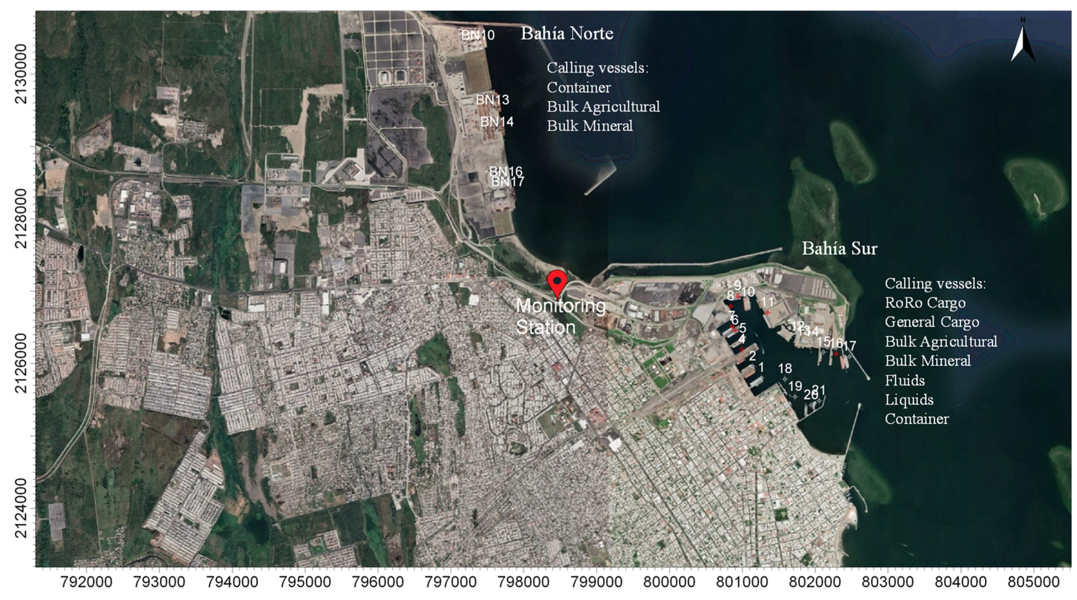
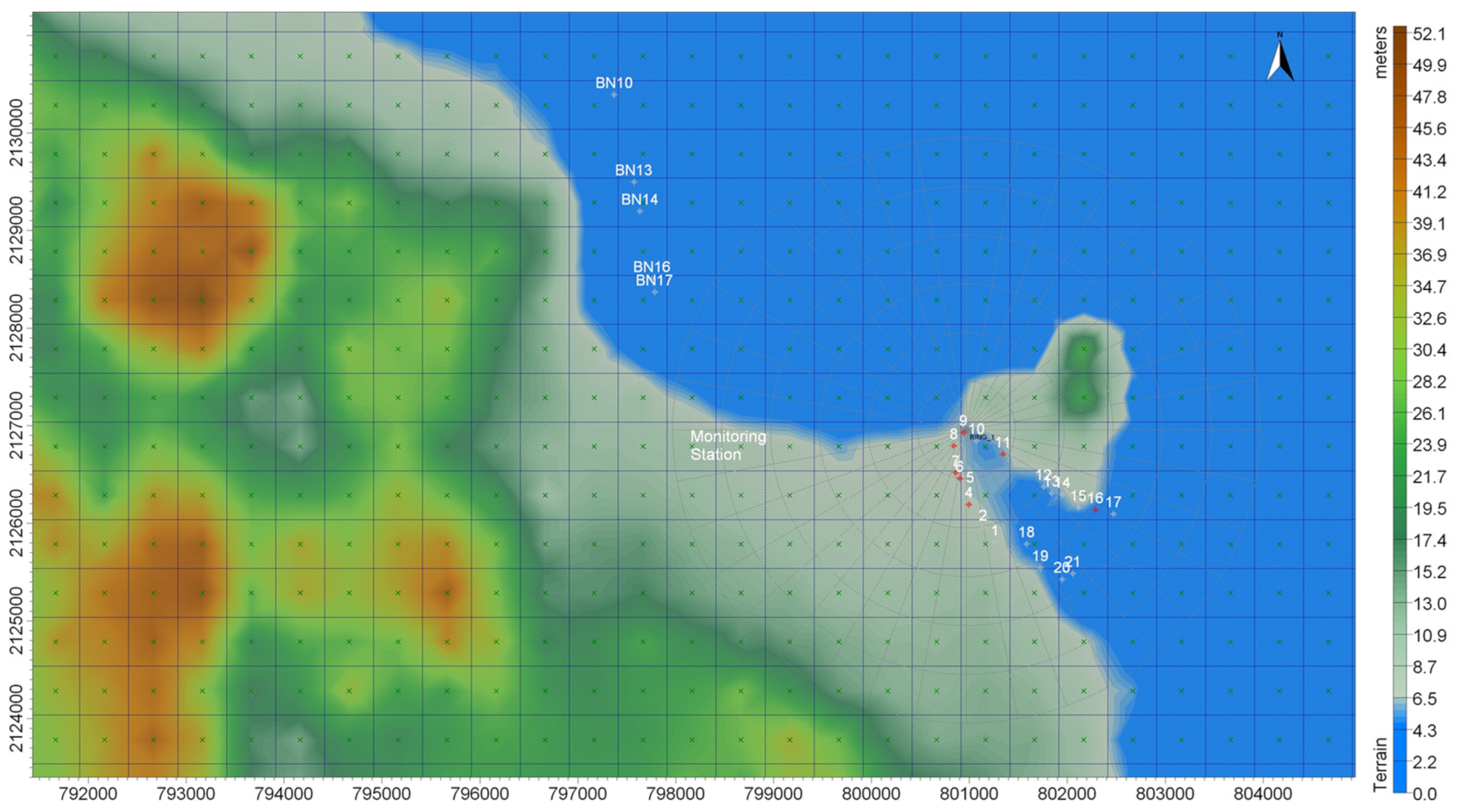
2. Port of Veracruz
3. Methodology
3.1. Atmospheric Emission
3.2. Air Quality Modeling and Meteorology
4. Results and Discussion
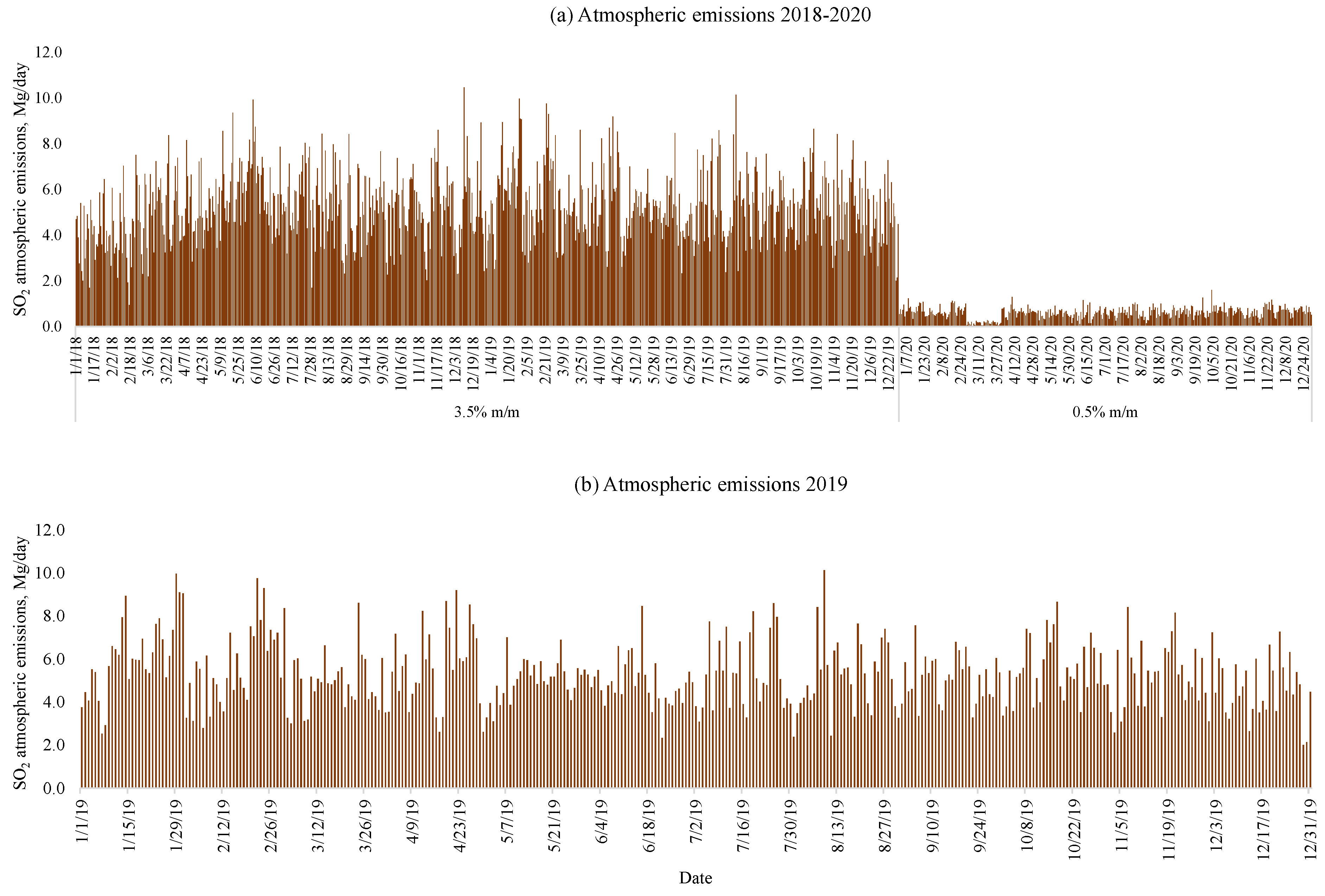
4.1. Atmospheric Emissions
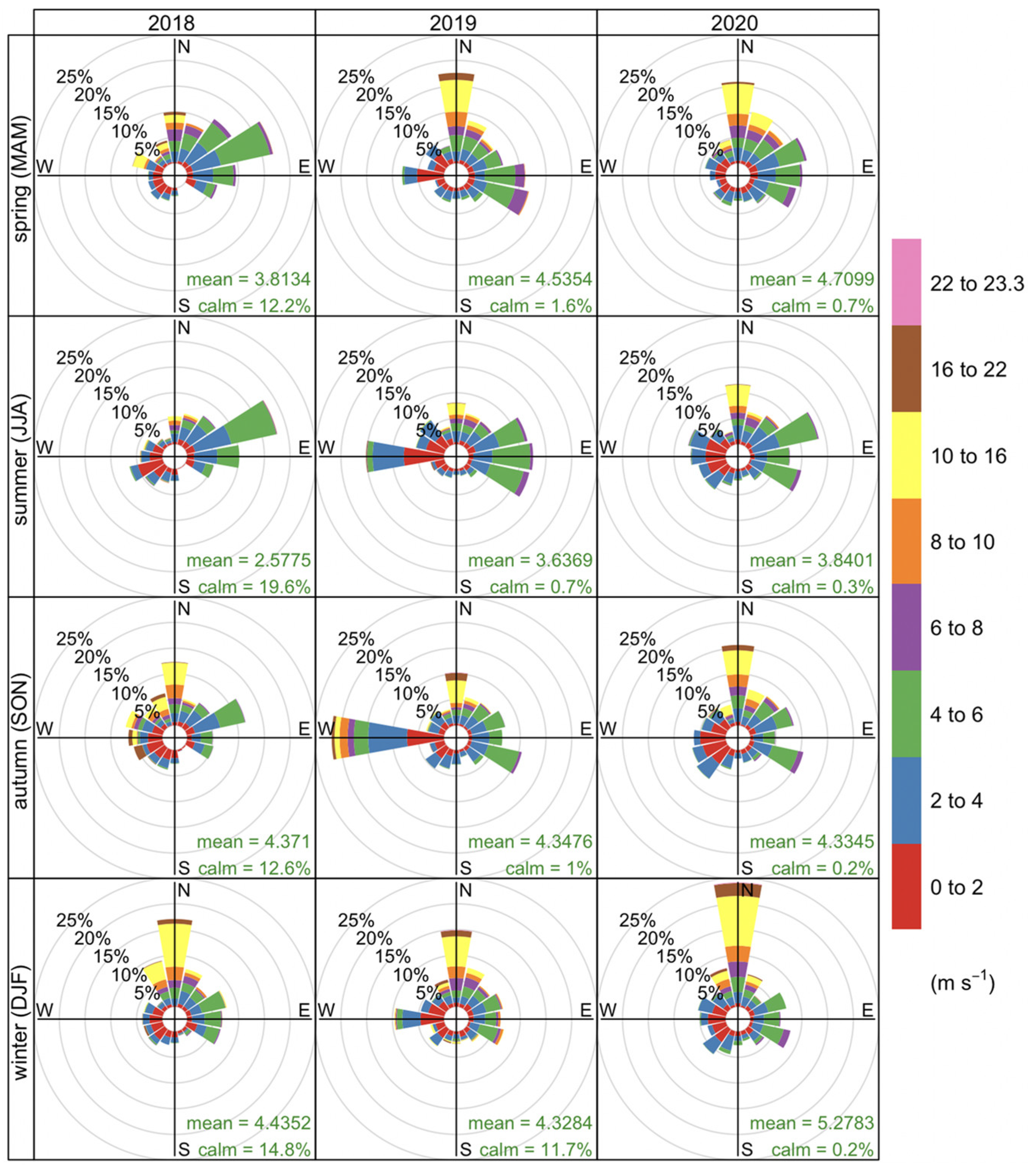
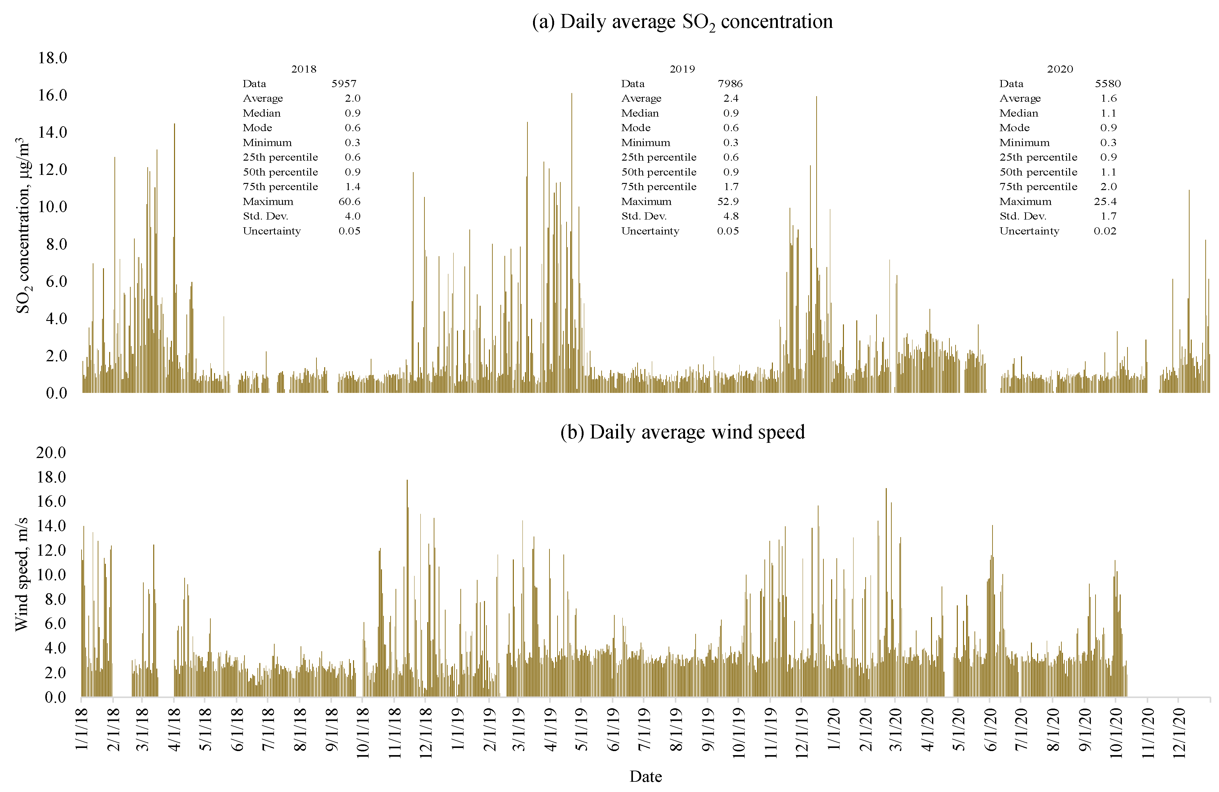
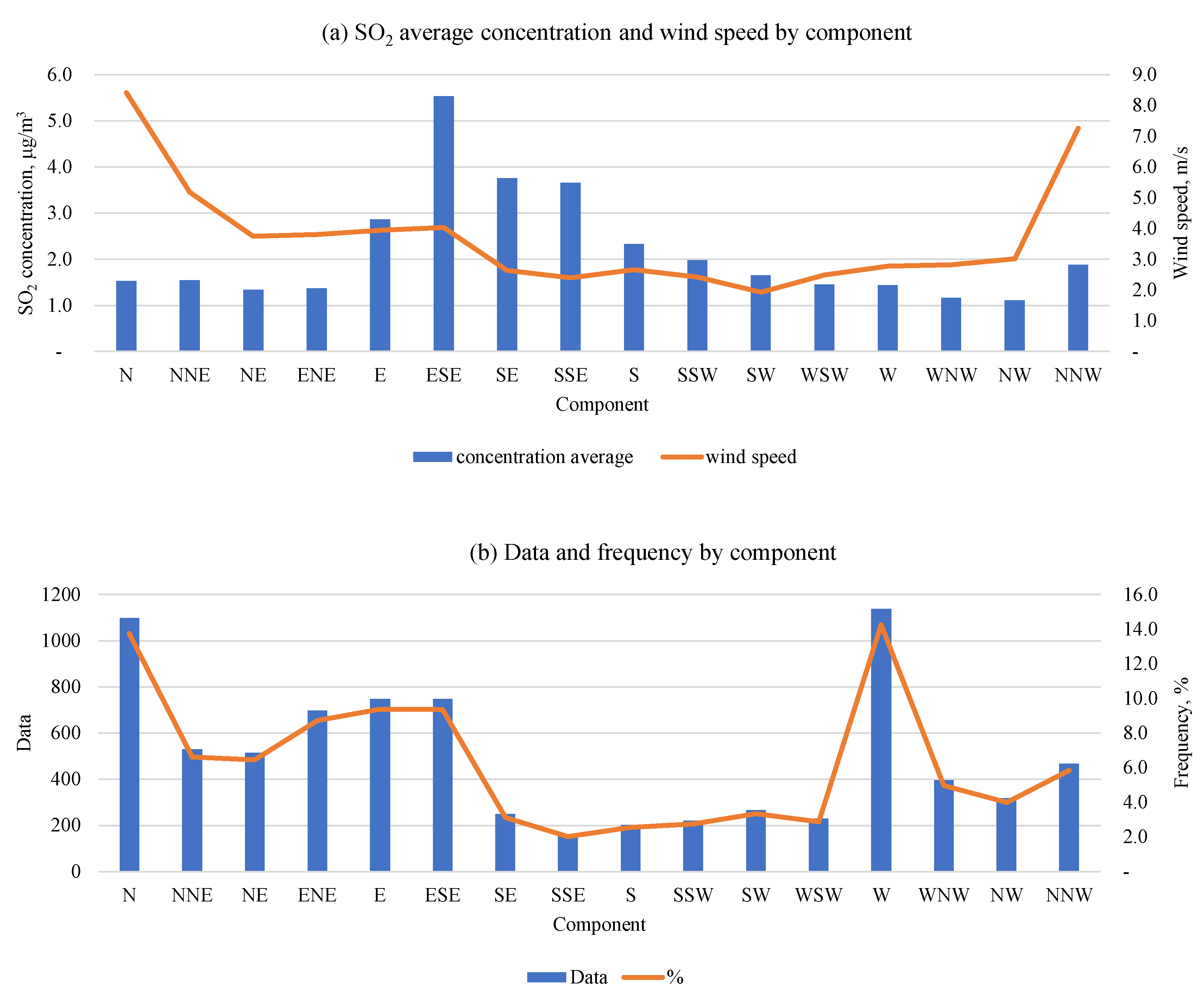
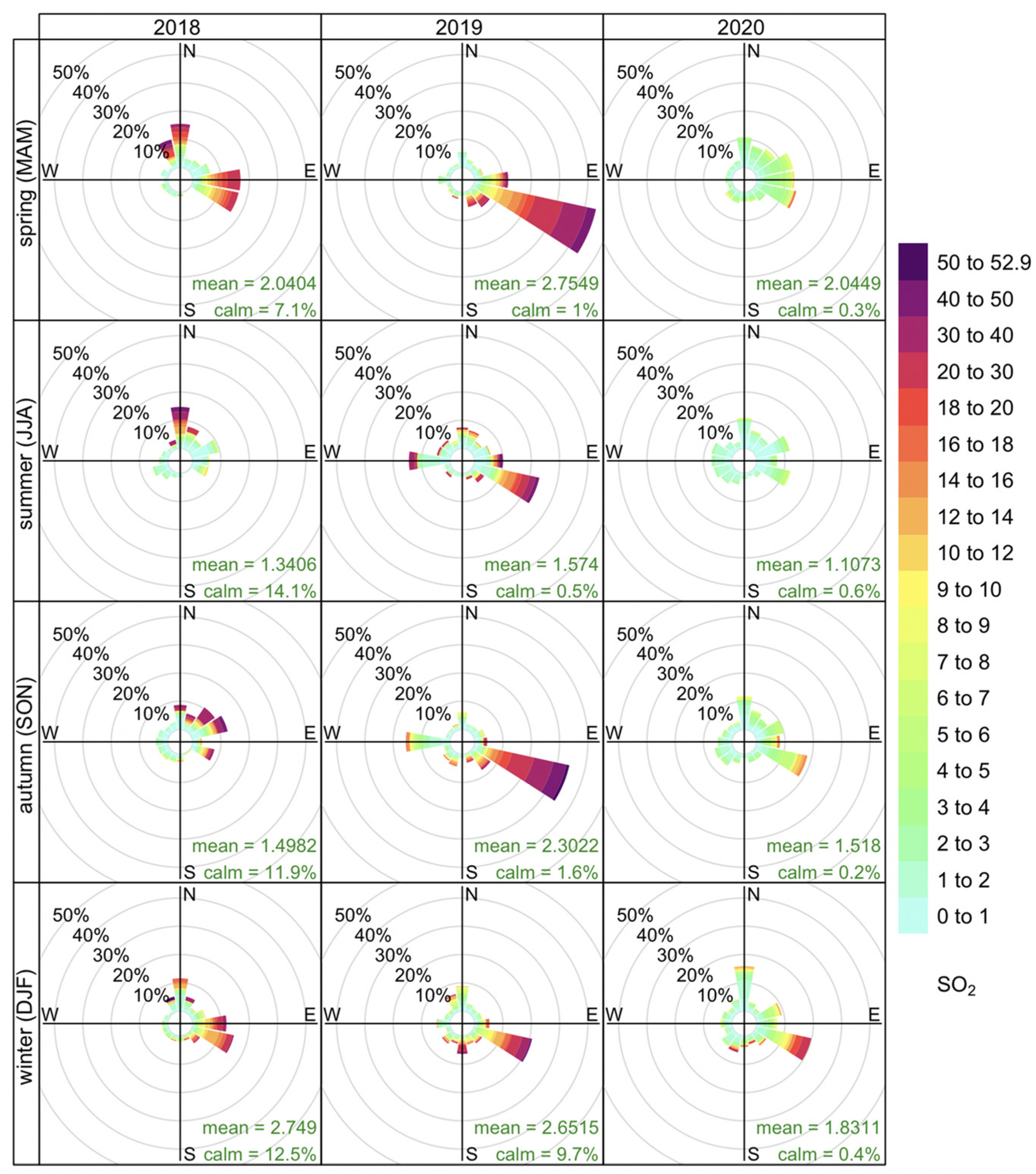
4.2. Air Quality and Meteorology
4.3. Modeling of Air Quality and Meteorology
5. Conclusions
6. Recommendations
7. Future Work
Author Contributions
Funding
Institutional Review Board Statement
Informed Consent Statement
Data Availability Statement
Acknowledgments
Conflicts of Interest
References
- Miola, A.; Ciuffo, B.; Giovine, E.; Marra, M. Regulating air emissions from ships: The state of the art on methodologies, technologies and policy options. In JRC Reference Report; Institute for Environment and Sustainability; European Commission: Ispra, Italy, 2010; Available online: https://publications.jrc.ec.europa.eu/repository/handle/JRC60732 (accessed on 7 March 2022).
- Davis, D.D.; Grodzinsky, G.; Kasibhatla, P.; Crawford, J.; Chen, G.; Liu, S.; Bandy, A.; Thornton, D.; Guan, H.; Sandholm, S. Impact of Ship Emissions on Marine Boundary Layer NOx and SO2 Distributions over the Pacific Basin. Geophys. Res. Lett. 2001, 28, 235–238. [Google Scholar] [CrossRef]
- Isaksson, J.; Persson, T.A.; Lindgren, E.S. Identification and assessment of ship emissions and their effects in the harbour of Goteborg, Sweden. Atmos. Environ. 2001, 35, 3659–3666. [Google Scholar] [CrossRef]
- Kesgin, U.; Vardar, N. A study on exhaust gas emissions from ships in Turkish Straits. Atmos. Environ. 2001, 35, 1863–1870. [Google Scholar] [CrossRef]
- Dong, C.; Huan, K.-L.; Chen, C.-W.; Lee, C.-W.; Lin, H.-Y.; Chen, C.-F. Estimation of Air Pollutants Emission from Shipping in the Kaohsiung Harbor Area. Aerosol Air Qual. Res. 2002, 2, 31–40. [Google Scholar] [CrossRef] [Green Version]
- Entec UK Limited; European Commission Directorate General Environment. Quantification of Emissions from Ships Associated with Ship Movements between Ports in the European Community; European Commission Directorate General Environment: Cheshire, UK, 2002. [Google Scholar]
- Georgakaki, A.; Coffey, R.A.; Lock, G.; Sorenson, S.C. Transport and Environment Database System (TRENDS): Maritime air pollutant emission modelling. Atmos. Environ. 2005, 38, 2357. [Google Scholar] [CrossRef] [Green Version]
- Delft. Greenhouse Gas Emissions for Shipping and Implementation Guidance for the Marine Fuel Sulphur Directive; Delft CE; Germanischer Lloyd, MARINTEK, Det Norske Veritas: Delft, The Netherlands, 2006; Available online: https://www.verifavia.com/bases/ressource_pdf/198/118098.pdf (accessed on 7 August 2022).
- Wang, C.; Corbett, J.J.; Firestone, J. Modeling Energy Use and Emissions from North American Shipping: Application of the Ship Traffic, Energy, and Environment Model. Environ. Sci. Technol. 2007, 41, 3226. [Google Scholar] [CrossRef]
- Yang, D.-Q.; Kwan, S.H.; Lu, T.; Fu, Q.-Y.; Cheng, J.-M.; Streets, D.G.; Wu, Y.-M.; Li, J.-J. An Emission Inventory of Marine Vessels in Shanghai in 2003. Environ. Sci. Technol. 2007, 41, 5183. [Google Scholar] [CrossRef]
- Starcrest. The Port of Los Angeles: Inventory of Air Emissions for Calendar Year 2020; APP#201113-540A; Starcrest Consulting Group: Poulsbo, WA, USA, 2021; Available online: https://www.portoflosangeles.org/environment/air-quality/air-emissions-inventory (accessed on 7 August 2022).
- Capaldo, K.; Corbett, J.J.; Kasibhatla, P.; Fischbeck, P.; Pandis, S.N. Effects of ship emissions on Sulphur cycling and radiative climate forcing over the ocean. Nature 1999, 400, 743–746. [Google Scholar] [CrossRef]
- Corbett, J.J.; Fishbeck, P.S.; Pandis, S.N. Global nitrogen and Sulphur inventories for oceangoing ships. J. Geophys. Res. 1999, 104, 3457–3470. [Google Scholar] [CrossRef]
- Corbett, J.; Winebrake, J.; Green, E.; Kasibhatla, P.; Eyring, V.; Lauer, A. Mortality from Ship Emissions: A Global Assessment. Environ. Sci. Technol. 2007, 41, 8512–8518. [Google Scholar] [CrossRef]
- Endresen, Ø.; Sørgard, E.; Sundet, J.K.; Dalsøren, S.B.; Isaksen, I.S.A.; Berglen, T.F.; Gravir, G. Emission from international sea transportation and environmental impact. J. Geophys. Res. 2003, 108, 4560. [Google Scholar] [CrossRef]
- Dalsøren, S.B.; Endresen, Ø.; Isaksen, I.S.A.; Gravir, G.; Sørgard, E. Environmental impacts of the expected increase in sea transportation, with a particular focus on oil and gas scenarios for Norway and northwest Russia. J. Geophys. Res. 2007, 112, D02310. [Google Scholar] [CrossRef]
- Tichavska, M.; Tova, B. Port-city exhaust emission model: An application to cruise and ferry operations in Las Palmas port. Transp. Res. A Policy Pract. 2015, 78, 347–360. [Google Scholar] [CrossRef]
- Mwase, N.S.; Ekstrom, A.; Jonson, J.E.; Svensson, E.; Jalkanen, J.-P.; Wichmann, J.; Molnár, P.; Stockfelt, L. Health Impact of Air Pollution from Shipping in the Baltic Sea: Effects of Different Spatial Resolutions in Sweden. Int. J. Environ. Res. Public Health 2020, 17, 7963. [Google Scholar] [CrossRef]
- Deniz, C.; Durmusoglu, Y. Estimating shipping emissions in the region of the Sea of Marmara, Turkey. Sci. Total Environ. 2008, 390, 255–261. [Google Scholar] [CrossRef]
- Carletti, S.; Latini, G.; Passerini, G. Air pollution and port operations: A case study and strategies to clean up. In Sustainable City VII (2 Volume Set); Transactions on Ecology and the Environment: Rome, Italy, 2012. [Google Scholar] [CrossRef]
- Castells, S.M.; Usabiaga, S.J.J.; Martínez, D.O.F.X. Manoeuvring and hotelling external costs: Enough for alternative energy sources? Marit. Policy Manag. 2014, 41, 42–60. [Google Scholar] [CrossRef] [Green Version]
- Chang, Y.-T.; Roh, Y.; Park, H. Assessing noxious gases of vessel operations in a potential Emission Control Area. Transp. Res. Part D 2014, 28, 91–97. [Google Scholar] [CrossRef]
- Dockery, D.W.; Pope, C.A.; Xu, X.; Spengler, J.D.; Ware, J.H.; Fay, M.E.; Ferris, B.G.; Speizer, F.E. An association between air pollution and mortality in six U.S. cities. N. Engl. J. Med. 1993, 329, 1753–1759. [Google Scholar] [CrossRef] [Green Version]
- Pope, C.A.; Burnett, R.T.; Thun, M.J.; Calle, E.E.; Krewski, D.; Ito, K.; Thurston, G.D. Lung cancer, cardiopulmonary mortality, and long-term exposure to fine particulate air pollution. JAMA 2002, 287, 1132–1141. [Google Scholar] [CrossRef]
- Pope, C.A., III; Ezzati, M.; Dockery, D.W. Fine-particulate air pollution and life expectancy in the United States. N. Engl. J. Med. 2009, 360, 376–386. [Google Scholar] [CrossRef] [Green Version]
- Bell, M.L.; Ebisu, K.; Peng, R.D.; Walker, J.; Samet, J.M.; Zeger, S.L.; Dominici, F. Seasonal and regional short-term effects of fine particles on hospital admissions in 202 US counties, 1999–2005. Am. J. Epidemiol. 2008, 168, 1301–1310. [Google Scholar] [CrossRef] [Green Version]
- Zanobetti, A.; Schwartz, J. The effect of fine and coarse particulate air pollution on mortality: A national analysis. Environ. Health Perspect. 2009, 117, 898–903. [Google Scholar] [CrossRef] [PubMed] [Green Version]
- UNCTAD. United Nations Conference on Trade and Development. In Proceedings of the Multi-Year Expert Meeting on Transport and Trade Facilitation: Maritime Transport and Climate Change Challenge, Geneva, Switzerland, 16–18 February 2009. Available online: https://unctad.org/meeting/multi-year-expert-meeting-transport-and-trade-facilitation (accessed on 7 March 2022).
- International Maritime Organization (IMO). 2019 Guidelines for Consistent Implementation of the 0.50% Sulphur Limit under MARPOL ANEX VI; Resolution MEPC.320(74); The Marine Environment Protection Committee: London, UK, 2019; Available online: https://wwwcdn.imo.org/localresources/en/KnowledgeCentre/IndexofIMOResolutions/MEPCDocuments/MEPC.320%2874%29.pdf (accessed on 7 August 2022).
- International Maritime Organization (IMO). 2020–Cutting Sulphur Oxide Emissions. Available online: https://www.imo.org/en/MediaCentre/HotTopics/Pages/Sulphur-2020.aspx (accessed on 9 August 2022).
- Vedachalam, S.; Baquerizo, N.; Dalai, A.K. Review on impacts of low sulfur regulations on marine fuels and compliance options. Fuel 2022, 310, 122243. [Google Scholar] [CrossRef]
- Cooper, D.A. Exhaust emissions from high-speed passenger ferries. Atmos. Environ. 2001, 35, 4189–4200. [Google Scholar] [CrossRef]
- Cooper, D.A. Exhaust emissions from ships at berth. Atmos. Environ. 2003, 37, 3817–3830. [Google Scholar] [CrossRef]
- Kasper, A.; Aufdenblatten, S.; Forss, A.; Burtscher, H. Particulate emissions from a low-speed marine diesel engine. Aerosol Sci. Techol. 2007, 41, 24–32. [Google Scholar] [CrossRef] [Green Version]
- Fridell, E.; Steen, E.; Peterson, K. Primary particles in ship emissions. Atmos. Environ. 2008, 42, 1160–1168. [Google Scholar] [CrossRef]
- Buhaug, Ø.; Corbett, J.J.; Endresen, Ø.; Eyring, V.; Faber, J.; Hanayama, S.; Lee, D.S.; Lee, D.; Lindstad, H.; Markowska, A.Z.; et al. Second IMO GHG Study 2009; International Maritime Organization (IMO): London, UK, 2009; Available online: https://wwwcdn.imo.org/localresources/en/OurWork/Environment/Documents/SecondIMOGHGStudy2009.pdf (accessed on 7 March 2022).
- Winnes, H.; Fridell, E. Particle emissions from ships: Dependence on fuel type. J. Air Waste Manag. 2012, 59, 1391–1398. [Google Scholar] [CrossRef] [PubMed]
- Chen, C.; Saikawa, E.; Comer, B.; Mao, X.; Ruthenford, D. Ship emission impacts on air quality and human health in the Pearl River Delta (PRD) region, China, in 2015, with projections to 2030. GeoHealth 2019, 3, 284–306. [Google Scholar] [CrossRef]
- Winebrake, J.J.; Corbett, J.J.; Green, E.H.; Lauer, A.; Eyring, V. Mitigating the health impacts of pollution from oceangoing shipping: An assessment of low-sulfur fuel mandates. Environ. Sci. Technol. 2009, 43, 4776–4782. [Google Scholar] [CrossRef] [Green Version]
- Viana, M.; Fann, N.; Tobías, A.; Querol, X.; Rojas-Rueda, D.; Plaza, A.; Aynos, G.; Conde, J.A.; Fernández, L.; Fernández, C. Environmental and health benefits from designating the marmara sea and the Turkish straits as an emission control area (ECA). Environ. Sci. Technol. 2015, 49, 3304–3313. [Google Scholar] [CrossRef]
- Corbett, J.J.; Winebrake, J.J.; Carr, E.W.; Jalkanen, J.-P.; Johansson, L.; Prank, M.; Sofiev, M. Health Impacts Associated with Delay of MARPOL Global Sulphur Standards. International Maritime Organization. Air Pollution and Energy Efficiency, 2016. Available online: https://wwwcdn.imo.org/localresources/en/MediaCentre/HotTopics/Documents/Finland%20study%20on%20health%20benefits.pdf (accessed on 7 March 2022).
- Sofiev, M.; Winebrake, J.J.; Johansson, L.; Carr, E.W.; Prank, M.; Soares, J.; Vira, J.; Kouznetsov, R.; Jalkanen, J.-P.; Corbett, J.J. Cleaner fuels for ships provide public health benefits with climate tradeoffs. Nat. Commun. 2018, 9, 406. [Google Scholar] [CrossRef] [PubMed] [Green Version]
- De Meyer, P.; Maes, F.; Volckaert, A. Emissions from international shipping in the Belgian Part of the North Sea and the Belgian Seaports. Atmos. Environ. 2008, 42, 196–206. [Google Scholar] [CrossRef]
- Matthias, V.; Aulinger, A.; Backes, A.; Bieser, J.; Geyer, B.; Quante, M.; Zeretzke, M. The impact of shipping emissions on air pollution in the greater North Sea region-Part 2: Scenarios for 2030. Atmos. Chem. Phys. 2016, 16, 759–776. [Google Scholar] [CrossRef] [Green Version]
- Lack, D.A.; Corbett, J.J.; Onasch, T.; Lerner, B.; Massoli, P.; Quinn, P.K.; Bates, T.S.; Covert, D.S.; Coffman, D.; Sierau, B.; et al. Particulate emissions from commercial shipping: Chemical, physical, and optical properties. J. Geophys. Res. 2009, 114, D00F04. [Google Scholar] [CrossRef] [Green Version]
- Paxian, A.; Eyring, V.; Beer, W.; Sausen, R.; Wright, C. Present-day and future global bottom-up ship emission inventories including polar routes. Environ. Sci. Technol. 2010, 44, 1333–1339. [Google Scholar] [CrossRef]
- Peng, X.; Wen, Y.; Wu, L.; Xiao, C.; Zhou, C.; Han, D. A sampling method for calculating regional ship emissions inventories. Transp. Res. D 2020, 89, 102617. [Google Scholar] [CrossRef]
- Fuentes, G.G.; Baldasano, R.J.M.; Sosa, E.R.; Granados, H.E.; Zamora, V.E.; Antonio, D.R.; Kahl, W.J. Estimation of atmospheric emissions from maritime activity in the Veracruz port, Mexico. J. Air Waste Manag. Assoc. 2021, 71, 934–948. [Google Scholar] [CrossRef]
- Fuentes, G.G.; Sosa, E.R.; Baldasano, R.J.M.; WKahl, J.D.; Granados, H.E.; Alarcón, J.A.L.; Antonio, D.R.E. Atmospheric Emissions in Ports Due to Maritime Traffic in Mexico. J. Mar. Sci. Eng. 2021, 9, 1186. [Google Scholar] [CrossRef]
- Fuentes, G.G.; Sosa, E.R.; Baldasano, R.J.M.; WKahl, J.D.; Antonio, D.R. Review of Top-Down Method to Determine Atmospheric Emissions in Port. Case of Study: Port of Veracruz, Mexico. J. Mar. Sci. Eng. 2022, 10, 96. [Google Scholar] [CrossRef]
- Granados, H.E.; López, A.X.; Vega, R.E.; Sosa, E.R.; Alarcón, J.A.L.; Fuentes, G.G.; Sámchez, A.P. Energy consumption and atmospheric emissions from refines petroleum in Mexico by 2030. Ing. Investig. Tecnol. 2020, XXII, 1–13. [Google Scholar] [CrossRef]
- Browning, L.; Hartley, S.; Bandemehr, A.; Gathright, K.; Miller, W. Demonstration of fuel switching on oceangoing vessels in the Gulf of Mexico. J. Air Waste Manag. Assoc. 2012, 62, 1093–1101. [Google Scholar] [CrossRef] [Green Version]
- Marmer, E.; Langmann, B. Impact of ship emissions on the Mediterranean summertime pollution and climate: A regional model study. Atmos. Environ. 2005, 39, 4659–4669. [Google Scholar] [CrossRef]
- Eyring, V.; Stevenson, D.S.; Lauer, A.; Dentener, F.J.; Butler, T.; Collins, W.J.; Ellingsen, K.; Gauss, M. Multi-model simulations of the impact of international shipping on Atmospheric Chemistry and Climate in 2000 and 2030. Atmos. Chem. Phys. 2007, 7, 757–780. [Google Scholar] [CrossRef] [Green Version]
- Lauer, A.; Eyring, V.; Hendricks, J.; Jöckel, P.; Lohmann, U. Global model simulations of the impact of ocean-going ships on aerosols, clouds, and the radiation budget. Atmos. Chem. Phys. 2007, 7, 5061–5079. [Google Scholar] [CrossRef] [Green Version]
- Abrutytė, E.; Zŭkauskaitė, A.; Mickevičienė, R.; Zabukas, V.; Paulauskienė, T. Evaluation of NOx emission and dispersion from marine ships in Klaipeda Sea port. J. Environ. Eng. Landsc. Manag. 2014, 22, 264–273. [Google Scholar] [CrossRef]
- Aksoyoglu, S.; Baltensperger, U.; Prévôt, A.S.H. Contribution of ship emissions to the concentration and deposition of air pollutants in Europe. Atmos. Chem. Phys. 2016, 16, 1895–1906. [Google Scholar] [CrossRef] [Green Version]
- Aulinger, A.; Matthias, V.; Zeretzke, M.; Bieser, J.; Quante, M.; Backes, A. The impact of shipping emissions on air pollution in the greater North Sea region–Part 1: Current emissions and concentrations. Atmos. Chem. Phys. 2016, 16, 739–758. [Google Scholar] [CrossRef] [Green Version]
- Broome, R.; Cope, M.; Goldsworthy, B.; Goldsworthy, L.; Emmerson, K.; Jegasothy, E.; Morgan, G. The mortality effect of ship-related fine particulate matter in the Sidney greater metropolitan region of NSW, Australia. Environ. Int. 2016, 87, 85–93. [Google Scholar] [CrossRef]
- Marelle, L.; Thomas, J.L.; Raut, J.; Law, K.S.; Jalkanen, J.; Johansson, L.; Roiger, A.; Schlager, H.; Kim, J.; Reiter, A.; et al. Air quality and radiative impacts of Arctic shipping emissions in the summertime in northern Norway: From the local to the regional scale. Atmos. Chem. Phys. 2016, 16, 2359–2379. [Google Scholar] [CrossRef] [Green Version]
- Chen, D.; Wang, X.; Nelson, P.; Li, Y.; Zhao, N.; Zhao, Y.; Lang, J.; Zhou, Y.; Guo, X. Ship emission inventory and its impact on the PM2.5 air pollution in Qingdao Port, North China. Atmos. Environ. 2017, 166, 351–361. [Google Scholar] [CrossRef]
- Chen, D.; Zhao, N.; Lang, J.; Zhou, Y.; Wang, X.; Li, Y.; Zhao, Y.; Guo, X. Contribution of ship emissions to the concentration of PM2.5: A comprehensive study using AIS data and WRF/Chem model in Bohai Rim Region, China. Sci. Total Environ. 2018, 610–611, 1476–1486. [Google Scholar] [CrossRef] [PubMed]
- Liu, Z.; Lu, X.; Feng, J.; Fan, Q.; Zhang, Y.; Yang, X. Influence of Ship Emissions on Urban Air Quality: A Comprehensive Study Using Highly Time-Resolved Online Measurements and Numerical Simulation in Shanghai. Environ. Sci. Technol. 2017, 51, 202–211. [Google Scholar] [CrossRef] [PubMed]
- Monteiro, A.; Russo, M.; Gama, C.; Borrego, C. How important are maritime emissions for the air quality: At European and national scale. Environ. Pollut. 2018, 242, 565–575. [Google Scholar] [CrossRef] [PubMed]
- Barregard, L.; Molnàr, P.; Jonson, E.J.; Stockfelt, L. Impact on Population Health of Baltic Shipping Emissions. Int. J. Environ. Res. Public Health 2019, 16, 1954. [Google Scholar] [CrossRef] [Green Version]
- Karl, M.; Jonson, J.E.; Uppstu, A.; Aulinger, A.; Prank, M.; Sofiev, M.; Jalkanen, J.-P.; Johansson, L.; Quante, M.; Matthias, V. Effects of ship emissions on air quality in the Baltic Sea region simulated with three different chemistry transport models. Atmos. Chem. Phys. 2019, 19, 7019–7053. [Google Scholar] [CrossRef] [Green Version]
- Tang, L.; Ramacher, M.; Moldanová, J.; Matthias, V.; Karl, M.; Johansson, L.; Jalkanen, J.P.; Yaramenka, K.; Aulinger, A.; Gustafsson, M. The impact of ship emissions on air quality and human health in the Gothenburg area-Part I: 2012 emissions. Atmos. Chem. Phys. 2020, 20, 7509–7530. [Google Scholar] [CrossRef]
- Schinas, O. The Issue of Air Emissions: Policy and Operational Considerations; Hamburg School of Busines Administration: 2013. Available online: https://www.researchgate.net/profile/Orestis-Schinas/publication/261833464_The_Issue_of_Air_Emissions_Policy_and_Operational_Considerations/links/621dd4f06051a1658201d9b6/The-Issue-of-Air-Emissions-Policy-and-Operational-Considerations.pdf (accessed on 7 March 2022).
- Fan, Y.V.; Perry, S.; Klemes, J.J.; Lee, C.T. A review on air emissions assessment: Transportation. J. Clean. Prod. 2018, 194, 673–684. [Google Scholar] [CrossRef]
- AirClim. Air Pollution from Ships. Sweden, 2011. Available online: https://www.cleanshipping.org/download/111128_Air%20pollution%20from%20ships_New_Nov-11(3).pdf (accessed on 7 August 2022).
- Smith, T.W.P.; Jalkanen, J.-P.; Anderson, B.A.; Corbett, J.J.; Faber, J.; Hanayama, S.; O’Keeffe, E.; Parker, S.; Johansson, L.; Aldous, L.; et al. Third IMO GHG Study 2014; International Maritime Organization (IMO): London, UK, 2015; Available online: https://wwwcdn.imo.org/localresources/en/OurWork/Environment/Documents/Third%20Greenhouse%20Gas%20Study/GHG3%20Executive%20Summary%20and%20Report.pdf (accessed on 7 August 2022).
- Intergovernmental Panel on Climate Change (IPCC). Impacts, Adaptation and Vulnerability. Cambridge, UK, and New York, USA. 2022. Available online: https://www.ipcc.ch/report/ar6/wg2/ (accessed on 5 August 2022).
- Olmer, N.; Comer, B.; Roy, B.; Mao, X.; Rutherford, D. Greenhouse Gas Emissions from Global Shipping, 2013–2015; The International Council on Clean Transportation: Washington, DC, USA, 2017; Available online: https://theicct.org/wp-content/uploads/2022/01/Global-shipping-GHG-emissions-2013-2015_Methodology_17102017_vF.pdf (accessed on 5 August 2022).
- Bailey, D.; Solomon, G. Pollution prevention at ports: Clearing the air. Environ. Impact Assess. Rev. 2004, 24, 749–774. [Google Scholar] [CrossRef]
- European Commission Directorate General Environment. Task 2a–Shore-Side Electricity; Final Report; Entec UK Limited: Cheshire, UK, 2005. [Google Scholar]
- European Commission Directorate General Environment. Task 2c–SO2 Abatement; Final Report; Entec UK Limited: Cheshire, UK, 2005. [Google Scholar]
- Sofia, D.; Gioiella, F.; Lotrecchiano, N.; Giuliano, A. Mitigation strategies for reducing air pollution. Environ. Sci. Pollut. Res. 2020, 27, 19226–19235. [Google Scholar] [CrossRef]
- Zhang, Y.; Yang, X.; Brown, R.; Yang, L.; Morawska, L.; Ristovski, Z.; Fu, Q.; Huang, C. Shipping emissions and their impacts on air quality in China. Sci. Total Environ. 2017, 581–582, 186–198. [Google Scholar] [CrossRef]
- Nunes, R.A.O.; Alvim-Ferraz, M.C.M.; Martis, F.G.; Calderay-Cayetano, F.; Durán-Granados, V.; Moreno-Gutiérrez, J.; Jalkanen, J.P.; Hannuniemi, H.; Sousa, S.I.V. Shipping emissions in the Iberian Peninsula and the impacts on air quality. Atmos. Chem. Phys. 2020, 20, 9473–9489. [Google Scholar] [CrossRef]
- Bucak, U.; Arslan, T.; Demirel, H.; Balin, A. Analysis of Strategies to Reduce Air Pollution from Vessels: A Case for Strait of Istanbul. JEMS 2021, 9, 22–30. [Google Scholar] [CrossRef]
- Andersson, K.; Brynolf, S.; Hansson, J.; Grahn, M. Criteria and Decision Support for A Sustainable Choice of Alternative Marine Fuels. Sustainability 2020, 12, 3623. [Google Scholar] [CrossRef]
- Khoder, M.I. Atmospheric conversion of sulfur dioxide to particulate sulfate and nitrogen oxide to particulate nitrate and gaseous nitric acid in an urban area. Chemosphere 2002, 49, 675–684. [Google Scholar] [CrossRef]
- Hassellöv, I.-M.; Turner, D.R.; Lauer, A.; Corbett, J.J. Shipping contributes to ocean acidification. Geophys. Res. Lett. 2013, 40, 2731–2736. [Google Scholar] [CrossRef] [Green Version]
- Wu, H.; Hong, S.; Hu, M.; Li, Y.; Yun, W. Assessment of the Factors Influencing Sulfur Dioxide Emissions in Shandong, China. Atmosphere 2022, 13, 142. [Google Scholar] [CrossRef]
- Beirle, S.; Hormann, C.; Penning de Vries, M.; Dorner, S.; Kern, C.; Wagner, T. Estimating the volcanic emission rate and atmospheric lifetime of SO2 from space: A case study for Kilauea volcano, Hawaii. Atmos. Chem. Phys. 2014, 14, 8309–8322. [Google Scholar] [CrossRef] [Green Version]
- Calkins, C.; Ge, C.; Wang, J.; Anderson, M.; Yang, K. Effects of meteorological conditions on sulfur dioxide air pollution in the North China plain during winters of 2006–2015. Atmos. Environ. 2016, 147, 296–309. [Google Scholar] [CrossRef]
- Sabatier, P.A. Top-down and bottom-up approaches to implementation research: A critical analysis and suggested synthesis. J. Publc Policy. 1986, 6, 21–48. [Google Scholar] [CrossRef]
- Endresen, Ø.; Bakke, J.; Sørgard, E.; Berglen, T.F.; Holmvang, P. Improved modelling of ship SO2 emissions–A fuel-based approach. Atmos. Environ. 2005, 39, 3621. [Google Scholar] [CrossRef]
- Endresen, Ø.; Sørgard, E.; Lee Behrens, H.; Brett, P.O.; Isaksen, I.S.A. A historical reconstruction of ships’ fuel consumption and emissions. J. Geophys. Res. 2007, 112, D12301. [Google Scholar] [CrossRef] [Green Version]
- Browning, L.; Bailey, K. Current Methodologies and Best Practices for Preparing Port Emission Inventories; ICF Consulting: Fairfax, VA, USA; Environmental Protection Agency; Office of Policy: Washington, DC, USA, 2006. Available online: https://www3.epa.gov/ttnchie1/conference/ei15/session1/browning.pdf (accessed on 9 August 2022).
- Dentener, F.; Kinne, S.; Bond, T.; Boucher, O.; Cofala, J.; Generoso, S.; Ginoux, P.; Gong, S.; Hoelzemann, J.J.; Ito, A.; et al. Emissions of primary aerosol and precursor gases in the years 2000 and 1750 prescribed data-sets for AeroCom. Atmos. Chem. Phys. 2006, 6, 4321. [Google Scholar] [CrossRef] [Green Version]
- Miola, A.; Paccagnan, V.; Mannino, I.; Massarutto, A.; Perujo, A.; Turvani, M. External Costs of Transportation. Case Study: Maritime Transport; Institute for Environment and Sustainability; JRC European Commission: Ispra, Italy, 2009. [Google Scholar] [CrossRef]
- Jalkanen, J.-P.; Brink, A.; Kalli, J.; Pettersson, H.; Kukkoken, J.; Stipa, T. A modelling system for the exhaust emissions of marine traffic and its application in the Baltic Sea area. Atmos. Chem. Phys. 2009, 9, 9209–9223. [Google Scholar] [CrossRef] [Green Version]
- Yau, P.S.; Lee, S.C.; Corbett, J.J.; Wang, C.; Chen, Y.; Ho, F.K. Estimation of exhaust emissions from ocean-going vessels in Hong Kong. Sci. Total. Environ. 2012, 431, 299–306. [Google Scholar] [CrossRef] [PubMed]
- Huang, L.; Wen, Y.; Geng, X.; Zhou, C.; Xiao, C. Estimation and spatio-temporal analysis of ship exhaust in a port area. Ocean Eng. 2017, 140, 401–411. [Google Scholar] [CrossRef]
- Zhang, Y.; Gu, J.; Wang, W.; Peng, Y.; Wu, X.; Feng, X. Inland port vessel emissions inventory based on Ship Traffic Emission Assessment Model–Automatic Identification System. Adv. Mech. Eng. 2017, 9, 1687814017712878. [Google Scholar] [CrossRef]
- Jalkanen, J.-P.; Johansson, L.; Kukkoken, H.; Brink, A.; Kalli, J.; Stipa, A. Extension of an assessment model of ship traffic exhaust emissions for particulate matter and carbon dioxide. Atmos. Chem. Phys. 2012, 12, 2641–2659. [Google Scholar] [CrossRef]
- Johansson, L.; Jalkanen, J.-P.; Kukkoken, J. Global assessment of shipping emissions in 2015 on a high spatial and temporal resolution. Atmos. Environ. 2017, 167, 403–415. [Google Scholar] [CrossRef]
- Moreno, G.J.; Calderay, F.; Saborido, N.; Boile, M.; Rodríguez, V.R.; Durán, G.V. Methodologies for estimating shipping emissions and energy consumption: A comparative analysis of current methods. Energy 2015, 86, 603–616. [Google Scholar] [CrossRef]
- Lonati, G.; Cernuschi, S.; Sidi, S. Air quality impact assessment of at-berth ship emissions: Case-study for the project of a new freight port. Sci. Total Environ. 2010, 409, 192–200. [Google Scholar] [CrossRef]
- Kuzu, S.L.; Bilgili, L.; Kilic, A. Estimation and Dispersion analysis of shipping emissions in Bandirma Port, Turkey. Environ. Dev. Sustain. 2020, 23, 10288–10308. [Google Scholar] [CrossRef]
- Mocerino, L.; Murena, F.; Quaranta, F.; Toscano, D. A methodology for the design of an effective air quality monitoring network in port areas. Sci. Rep. 2020, 10, 300. [Google Scholar] [CrossRef] [Green Version]
- Roberts Bank Container Expansion Project. RWDI DeltaPort Third Berth. In CALPUFF Dispersion Model—Appendix D; Port of Vancouver: Vancouver, WA, USA, 2005; Available online: https://www.portvancouver.com/wp-content/uploads/2015/03/techvols_tv8_appendix_d_calpuff_jan05.pdf (accessed on 7 March 2022).
- Jahangiri, S.; Nikolova, N.; Tenekedjiev, K. Application of a Developed Dispersion Model to Port of Brisbane. Am. J. Environ. Sci. 2018, 14, 156–169. [Google Scholar] [CrossRef]
- Murena, F.; Mocerino, L.; Quaranta, F.; Toscano, D. Impact on air quality of cruise ship emissions in Naples, Italy. Atmos. Environ. 2018, 187, 70–83. [Google Scholar] [CrossRef]
- Berths 97-109. China ShippingContainer Terminal Project. Port Los Angeles, USA. 2019. Available online: https://kentico.portoflosangeles.org/getmedia/477b7424-414b-4a7b-b796-ed8f91decab5/CS_Appendix_B2_Air_Dispersion_Modeling_FSEIR (accessed on 7 March 2022).
- Pan, K.; Lim, M.Q.; Kraft, M.; Mastorakos, E. Development of a moving point source model for shipping emission dispersion modeling in EPISODE -City Chem v.1.3. Geosci. Model. Dev. 2021, 14, 4509–4534. [Google Scholar] [CrossRef]
- Bai, S.; Wen, Y.; He, L.; Liu, Y.; Zhang, Y.; Yu, Q.; Ma, W. Single-Vessel Plume Dispersion Simulation: Method and a Case Study Using CALPUFF in the Yantian Port Area, Shenzhen (China). Int. J. Environ. Res. Public Health 2020, 17, 7831. [Google Scholar] [CrossRef]
- Scire, J.S.; Strimaitis, D.G.; Yamartino, R.J. A User’s Guide for the CALPUFF Dispersion Model; Version 5; Earth Tech, Inc.: Concord, MA, USA, 2000; Available online: http://www.src.com/calpuff/download/CALPUFF_UsersGuide.pdf (accessed on 27 July 2022).
- Entec UK Limited. Defra, UK Ship Emissions Inventory. Final Report, England; 2010. Available online: https://uk-air.defra.gov.uk/assets/documents/reports/cat15/1012131459_21897_Final_Report_291110.pdf (accessed on 7 August 2022).
- Skamarock, W.C.; Klemp, J.B.; Dudhia, J.; Gill, D.O.; Liu, Z.; Berner, J.; Wang, W.; Powers, J.G.; Duda, M.G.; Barker, D.M.; et al. A Description of the Advanced Research WRF Version 4. NCAR Tech. Notes 2021, NCAR/TN-556+STR. [Google Scholar] [CrossRef]
- World Health Organization (WHO). Global Air Quality Guidelines: Particulate Matter (PM2.5 and PM10), Ozone, Nitrogen Dioxide, Sulfur Dioxide and Carbon Monoxide. License CC BY-NC-SA 3.0IGO. 2021. Available online: https://apps.who.int/iris/handle/10665/345329 (accessed on 29 July 2022).
- Norma Oficial Mexicana (NOM). NOM-020-SSA1-2019. Salud Ambiental. Criterio Para Evaluar la Calidad del Aire con Res-pecto a Dióxido de Azufre (SO2). Diario Oficial de la Federación, México. 2019. Available online: https://www.dof.gob.mx/nota_detalle.php?codigo=5568395&fecha=20/08/2019#gsc.tab=0 (accessed on 29 July 2022).
- Stein, A.F.; Draxler, R.R.; Rolph, G.D.; Stunder, B.J.B.; Cohen, M.D.; Ngan, F. NOAA’s HYSPLIT atmospheric transport and dispersion modeling system. Bull. Am. Meteorol. Soc. 2015, 96, 2059–2077. [Google Scholar] [CrossRef]
- Rolph, G.; Stein, A.; Stunder, B. Real-time Environmental Applications and Display System: READY. Environ. Model. Softw. 2017, 95, 210–228. [Google Scholar] [CrossRef]
- United States Environmental Protection Agency (USEPA). Air Monitoring Methods–Criteria Pollutants, and Quality Assurance, USA. 2022. Available online: https://www.epa.gov/amtic/air-monitoring-methods-criteria-pollutants (accessed on 7 August 2022).
- Norma Oficial Mexicanay (NOM). NOM-156-SEMARNAT-2012. Establecimiento y Operación de Sistemas de Monitoreo de Calidad del Aire. Ciudad de México, México; 2012. Available online: https://www.dof.gob.mx/nota_detalle.php?codigo=5259464&fecha=16/07/2012#gsc.tab=0 (accessed on 25 July 2022).
- VER. Puerto de Veracruz, México. 2022. Available online: https://www.puertodeveracruz.com.mx/wordpress/estadisticas-2/resumen-historico/ (accessed on 7 March 2022).
- Trozzi, C. Emission Estimate Methodology for Maritime Navigation; Techne Consulting srl: Rome, Italy, 2010. Available online: https://www3.epa.gov/ttnchie1/conference/ei19/session10/trozzi.pdf (accessed on 25 February 2022).
- Cooper, D.; Gustafsson, T. Methodology for Calculating Emissions from Ships: 2. Emission Factors for 2004 Reporting. Sweden. 2004. Available online: https://www.diva-portal.org/smash/get/diva2:1117169/FULLTEXT01.pdf (accessed on 25 February 2022).
- NCEP. National Centers for Environmental Prediction/National Weather Service/NOAA/U.S. Department of Commerce. 2015, update daily. In NCEP GDAS/FNL 0.25 Degree Global Tropospheric Analyses and Forecast Grids; Research Data Archive at National Center for Atmospheric Research, Computational and Information Systems Laboratory: Boulder, CO, USA, 2015. [Google Scholar] [CrossRef]
- Baldasano, J.M.; Soret, A.; Guevara, M.; Martínez, F.; Gassó, S. Integrated assessment of air pollution using observations and modeling in Santa Cruz de Tenerife (Canary Islands). Sci. Total. Environ. 2014, 473–474, 576–588. [Google Scholar] [CrossRef] [PubMed]
- Kahl, J.; Bravo-Álvarez, H.; Sosa-Echeverría, R.; Sánchez-Álvarez, P.; Alarcón-Jiménez, A.L.; Soto-Ayala, R. Characterization of atmospheric transport to the El Tajín Archaeological Zone in Veracruz, Mexico. Atmosfera 2007, 20, 359–371. Available online: https://www.scielo.org.mx/scielo.php?script=sci_arttext&pid=S0187-62362007000400004 (accessed on 3 October 2022).


| Type of Ship | Type of Cargo | Ships Calling | GT Average | Hoteling, Time (h) | Frequency | ||||||||
|---|---|---|---|---|---|---|---|---|---|---|---|---|---|
| 2018 | 2019 | 2020 | 2018 | 2019 | 2020 | 2018 | 2019 | 2020 | 2018 | 2019 | 2020 | ||
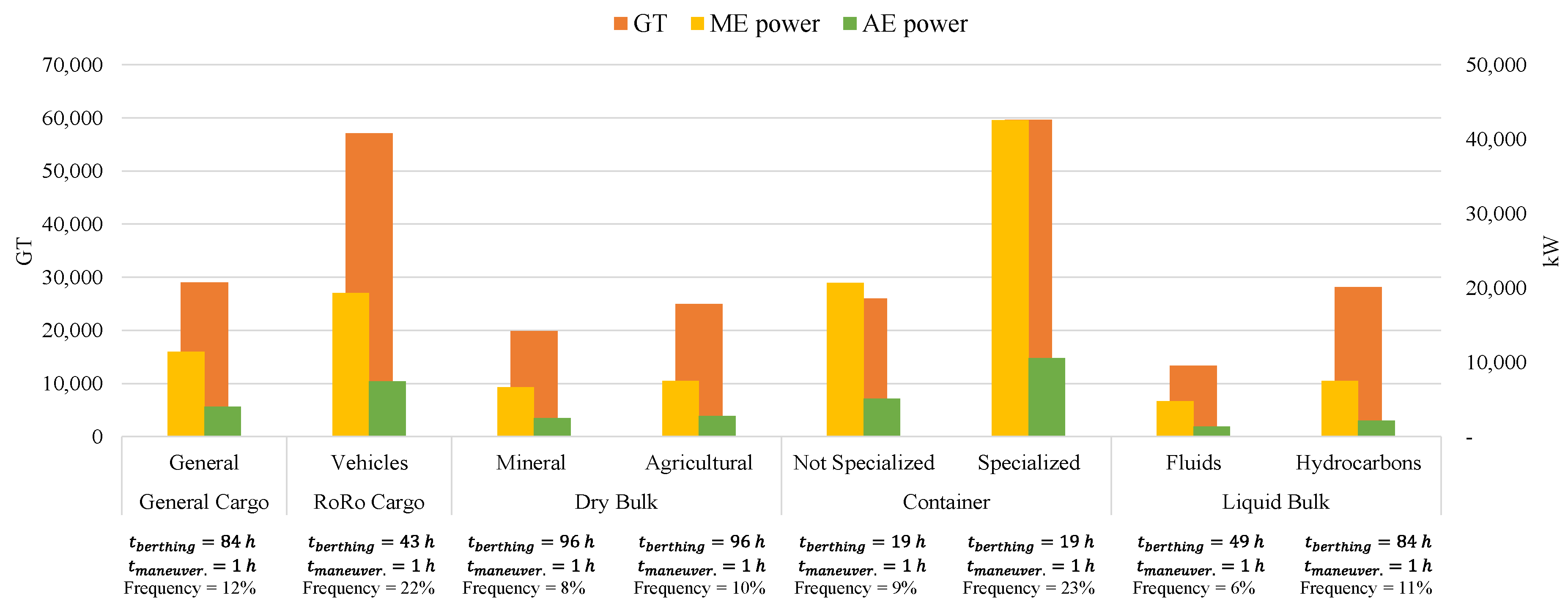
| General Cargo | General | 340 | 358 | 296 | 27,298 | 28,979 | 30,672 | 85 | 88 | 75 | 11% | 11% | 12% |
| RoRo Cargo | Vehicles | 267 | 230 | 178 | 56,373 | 57,407 | 57,329 | 42 | 45 | 42 | 22% | 22% | 22% |
| Dry Bulk | Mineral | 172 | 125 | 148 | 20,343 | 20,314 | 19,182 | 102 | 92 | 94 | 8% | 8% | 8% |
| Agricultural | 228 | 236 | 223 | 24,999 | 24,589 | 25,284 | 170 | 155 | 158 | 10% | 9% | 10% | |
| Container | Non-Specialized | 171 | 168 | 110 | 28,441 | 27,031 | 22,486 | 21 | 21 | 16 | 11% | 10% | 9% |
| Specialized | 456 | 494 | 532 | 59,293 | 60,435 | 59,153 | 19 | 21 | 17 | 23% | 23% | 23% | |
| Liquid Bulk | Fluids | 172 | 177 | 186 | 11,757 | 13,807 | 14,479 | 32 | 54 | 61 | 5% | 5% | 6% |
| Hydrocarbons | 174 | 208 | 188 | 29,093 | 28,367 | 26,839 | 70 | 88 | 94 | 11% | 11% | 11% | |
| Total | 1980 | 1996 | 1861 | 257,597 | 260,929 | 255,424 | 541 | 564 | 557 | 100% | 100% | 100% | |
| Reference | Height, m | Diameter, m | Exhaust Gas Velocity, m/s | Exhaust Gas Temperature, K |
|---|---|---|---|---|
| [103] | 36.5 | 1.5 | 5.0 | 373.0 |
| [104] | 20.0 | 0.8 | 25.0 | 540.0 |
| [105] | 40.0 | 1.0 | 10.0 | 573.0 |
| [106] | 44.0 | 0.5 | 7.5 | 583.0 |
| [107] | 30.0 | 0.5 | 20.0 | 573.0 |
| Event | Day | Air Quality Monitoring Station | Component | Bahía Sur Emissions, kg/day | ||
|---|---|---|---|---|---|---|
| SO2 Concentration, μg/m3 | Wind Speed, m/s | Wind Direction, Degrees | ||||
| 1 | 8/3/19 | 11.6 | 3.3 | 90.0 | East | 3111 |
| 2 | 9/3/19 | 14.5 | 2.6 | 90.0 | East | 3186 |
| 3 | 25/9/19 | 12.4 | 2.7 | 112.5 | East-southeast | 6187 |
| 4 | 30/3/19 | 12.0 | 2.8 | 112.5 | East-southeast | 3618 |
| 5 | 4/4/19 | 10.7 | 1.9 | 112.5 | East-southeast | 7184 |
| 6 | 6/4/19 | 11.3 | 2.5 | 112.5 | East-southeast | 5670 |
| 7 | 7/4/19 | 10.1 | 2.8 | 112.5 | East-southeast | 6212 |
| 8 | 10/4/19 | 11.3 | 3.0 | 112.5 | East-southeast | 4889 |
| 9 | 11/4/19 | 9.0 | 2.0 | 112.5 | East-southeast | 4875 |
| 10 | 16/4/19 | 9.2 | 2.2 | 112.5 | East-southeast | 3275 |
| 11 | 21/4/19 | 16.1 | 1.9 | 112.5 | East-southeast | 5488 |
| 12 | 28/4/19 | 10.0 | 2.2 | 112.5 | East-southeast | 6967 |
| Dock | Type | Days | |||||||||||
|---|---|---|---|---|---|---|---|---|---|---|---|---|---|
| 8/3/19 | 9/3/19 | 25/3/19 | 30/3/19 | 4/4/19 | 6/4/19 | 7/4/19 | 10/4/19 | 11/4/19 | 16/4/19 | 21/4/19 | 28/4/19 | ||
| 1 | General, RoRo Cargo | - | 287 | 870 | 45 | 45 | 45 | - | 90 | 742 | 147 | 1186 | - |
| 2 | General | 57 | 57 | 114 | 61 | 92 | 98 | 355 | 256 | - | 125 | 229 | - |
| 4 | General, Dry Bulk | 281 | 281 | 301 | 49 | 516 | 934 | 934 | 387 | 431 | 44 | 498 | 451 |
| 5 | General, Dry Bulk | 92 | - | - | 301 | - | - | - | 562 | 562 | 289 | 1240 | - |
| 6 | Dry Bulk | - | - | 553 | 320 | 1246 | 89 | 89 | 89 | 241 | 758 | 617 | 771 |
| 7 | Container, RoRo Cargo | - | 276 | 1361 | 361 | - | 2231 | 1240 | 48 | 611 | 235 | 684 | 1659 |
| 8 | Dry Bulk | 569 | 569 | 206 | 682 | 469 | 469 | 681 | 469 | 218 | - | 393 | 545 |
| 9 | Cement | 354 | 354 | - | - | 271 | 538 | 703 | 142 | 745 | - | 343 | 569 |
| 11 | Container | 1346 | 338 | 1090 | 972 | 2922 | 338 | 972 | 2124 | 916 | 1078 | - | 1907 |
| 16 | Liquid Bulk | 412 | 1025 | 1692 | 827 | 1624 | 927 | 1238 | 721 | 410 | 600 | 299 | 1064 |
| Total | 3111 | 3186 | 6187 | 3618 | 7184 | 5670 | 6212 | 4889 | 4875 | 3275 | 5488 | 6967 | |
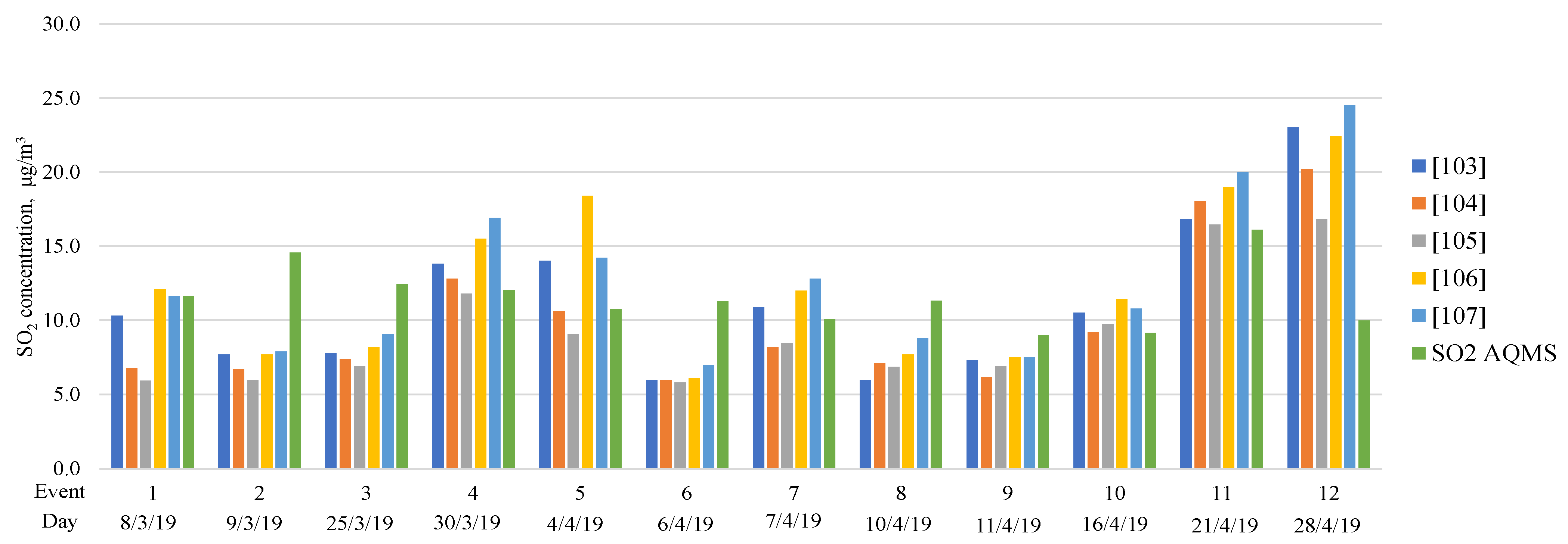
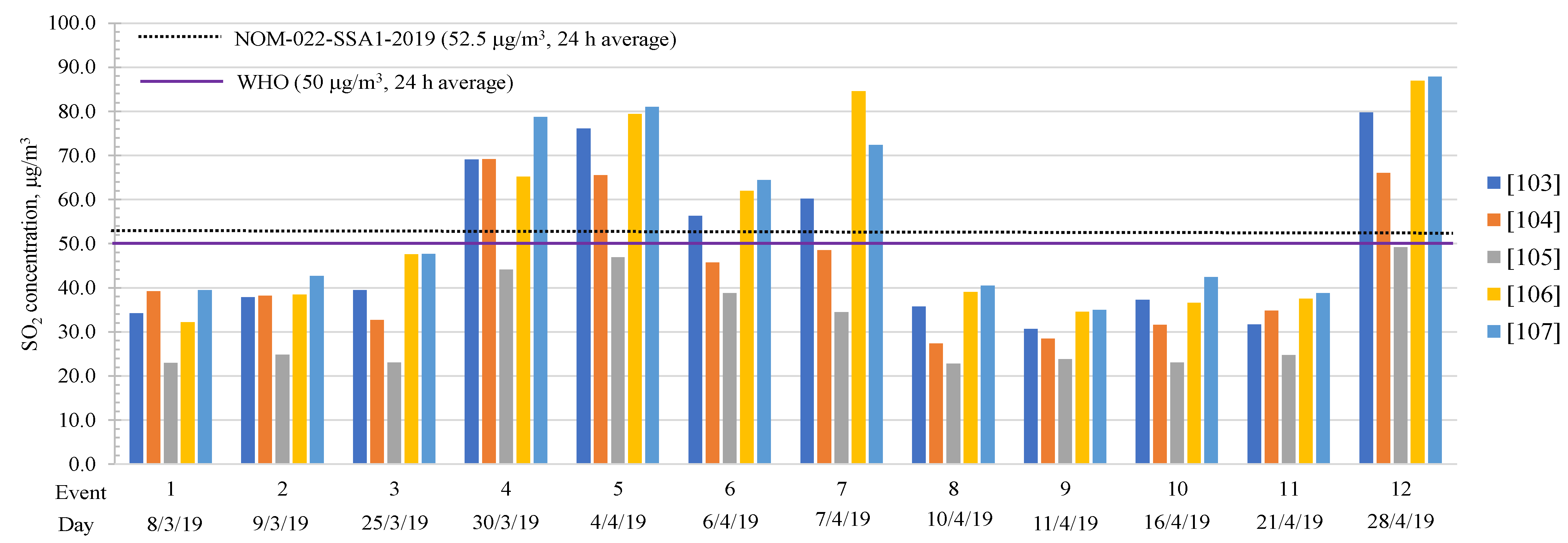
| Event | Day | Wind Speed, m/s | Wind Direction, Degrees | Wind Component | Bahía Sur Emissions, kg/day | AQMS μg/m3 | Modeling SO2 Concentration at 24 h Average, μg/m3 | ||||
|---|---|---|---|---|---|---|---|---|---|---|---|
| [103] | [104] | [105] | [106] | [107] | |||||||
| 1 | 8/3/19 | 3.3 | 90.0 | East | 3111 | 11.61 | 10.30 | 6.80 | 5.94 | 12.10 | 11.60 |
| 2 | 9/3/19 | 2.6 | 90.0 | East | 3186 | 14.55 | 7.70 | 6.70 | 6.00 | 7.70 | 7.90 |
| 3 | 25/3/19 | 2.7 | 112.5 | East-southeast | 6187 | 12.42 | 7.80 | 7.40 | 6.90 | 8.20 | 9.10 |
| 4 | 30/3/19 | 2.8 | 112.5 | East-southeast | 3618 | 12.04 | 13.80 | 12.80 | 11.79 | 15.50 | 16.90 |
| 5 | 4/4/19 | 1.9 | 112.5 | East-southeast | 7184 | 10.74 | 14.00 | 10.60 | 9.10 | 18.40 | 14.20 |
| 6 | 6/4/19 | 2.5 | 112.5 | East-southeast | 5670 | 11.27 | 6.00 | 6.00 | 5.83 | 6.10 | 7.00 |
| 7 | 7/4/19 | 2.8 | 112.5 | East-southeast | 6212 | 10.08 | 10.90 | 8.20 | 8.45 | 12.00 | 12.80 |
| 8 | 10/4/19 | 3.0 | 112.5 | East-southeast | 4889 | 11.32 | 6.00 | 7.10 | 6.88 | 7.70 | 8.80 |
| 9 | 11/4/19 | 2.0 | 112.5 | East-southeast | 4875 | 9.02 | 7.30 | 6.20 | 6.94 | 7.50 | 7.50 |
| 10 | 16/4/19 | 2.2 | 112.5 | East-southeast | 3275 | 9.18 | 10.50 | 9.20 | 9.74 | 11.40 | 10.80 |
| 11 | 21/4/19 | 1.9 | 112.5 | East-southeast | 5488 | 16.10 | 16.80 | 18.00 | 16.46 | 19.00 | 20.00 |
| 12 | 28/4/19 | 2.2 | 112.5 | East-southeast | 6967 | 9.99 | 23.00 | 20.20 | 16.80 | 22.40 | 24.50 |
Publisher’s Note: MDPI stays neutral with regard to jurisdictional claims in published maps and institutional affiliations. |
© 2022 by the authors. Licensee MDPI, Basel, Switzerland. This article is an open access article distributed under the terms and conditions of the Creative Commons Attribution (CC BY) license (https://creativecommons.org/licenses/by/4.0/).
Share and Cite
Fuentes García, G.; Echeverría, R.S.; Reynoso, A.G.; Baldasano Recio, J.M.; Rueda, V.M.; Retama Hernández, A.; Kahl, J.D.W. Sea Port SO2 Atmospheric Emissions Influence on Air Quality and Exposure at Veracruz, Mexico. Atmosphere 2022, 13, 1950. https://doi.org/10.3390/atmos13121950
Fuentes García G, Echeverría RS, Reynoso AG, Baldasano Recio JM, Rueda VM, Retama Hernández A, Kahl JDW. Sea Port SO2 Atmospheric Emissions Influence on Air Quality and Exposure at Veracruz, Mexico. Atmosphere. 2022; 13(12):1950. https://doi.org/10.3390/atmos13121950
Chicago/Turabian StyleFuentes García, Gilberto, Rodolfo Sosa Echeverría, Agustín García Reynoso, José María Baldasano Recio, Víctor Magaña Rueda, Armando Retama Hernández, and Jonathan D. W. Kahl. 2022. "Sea Port SO2 Atmospheric Emissions Influence on Air Quality and Exposure at Veracruz, Mexico" Atmosphere 13, no. 12: 1950. https://doi.org/10.3390/atmos13121950