Quantifying a Reliable Framework to Estimate Hydro-Climatic Conditions via a Three-Way Interaction between Land Surface Temperature, Evapotranspiration, Soil Moisture

Abstract

Distributed hydrological models can be suitable choices for predicting the spatial distribution of water and energy fluxes if the conceptual relationships between the components are defined appropriately. Therefore, an innovative approach has been developed using a simultaneous formulation of bulk heat transfer theory, energy budgeting, and water balance as an integrated hydrological model, i.e., the Monthly Continuous Semi-Distributed Energy Water Balance (MCSD-EWB) model, to estimate land surface hydrological components. The connection between water and energy balances is established by evapotranspiration (ET), which is a function of soil moisture and land surface temperature (LST). Thus, the developed structure is based on a three-way coupling between ET, soil moisture, and LST. The LST is obtained via the direct solution of the energy balance equation, and the spatiotemporal distribution of ET is presented using the computed LST and soil moisture through the bulk transfer method and water balance. In addition to the LST computed using the MCSD-EWB model, the LST products of ERA5-Land and MODIS are also utilized as inputs. The results indicate the adequate performance of the model in simulating LST, ET, streamflow, and groundwater level. Furthermore, the developed model performs better by employing the ERA5-Land LST than by using the MODIS LST in estimating the components.

1. Introduction

Distributed hydrological models provide a suitable approach for understanding the spatiotemporal patterns of water and energy fluxes with the aim of managing water resources and consumption [1]. Nevertheless, it is possible to project the physical concept or systematic structure into a complex regression model if the conceptual relationship between the model’s components, such as soil moisture and evapotranspiration (ET), is not defined correctly [2]. Therefore, the simultaneous evaluation of water and surface energy balances as an integrated system is recommended in order to correctly define conceptual relationships between hydrological components and to investigate the watershed hydro-climatic conditions at the same time.

The main core of the relationship between water and surface energy balances is the ET mechanism [2,3]. This component includes evaporation from water bodies and land surfaces, canopy interception, the sublimation of snow and ice, plant transpiration, and any moist ground and vegetation surfaces [4]. One of the most important factors controlling the ET process is the land surface temperature (LST). In addition, LST affects the determination of soil moisture indirectly through ET. Therefore, LST is a key factor in modeling water and energy balances.

LST is mainly obtained from thermal infrared radiation (TIR) datasets and radiative temperature equations [5,6]. Since TIR is limited by atmospheric factors, such as water vapor and cloud cover [7,8], the estimated LST and thereby ET values may be discontinuous in watershed-scale and long-term hydrological modeling [9]. In addition, ignoring soil moisture as an available water resource in the ET computing process is another limitation of this approach [10]. On the other hand, in situ measurements of LST across large areas, except for a few points, are not practical because of the heterogeneity in surface characteristics [6]. To address the limitations of LST estimation, the energy-based approach is recommended by directly solving the energy balance equation implemented by remote sensing data [11]. In this regard, different energy-based land surface models (LSMs) have been developed to solve the energy and mass balances using sophisticated equations [12]. For example, some of the land surface models based on the direct solution of the surface energy balance are the Biosphere–Atmosphere Transfer Scheme (BATS) [13], simple biosphere model (SiB) [14], Mosaic land surface model [15], Noah land surface model [16], and Variable Infiltration Capacity (VIC) model. In these models, the LST is directly achieved from the closure of the energy balance equation using a numerical method. The mass transfer equation and computed LST are subsequently used to estimate ET by using the mean values of the surface layer variables and turbulent transfer principles. Although LSMs employ the energy–water equations system to estimate the surface hydrological components, the one-way solution of the system restricts their application due to misestimations under extremely dry and wet conditions. Therefore, an integrated framework is needed to simultaneously estimate the LST, soil moisture, and ET based on a mutual evaluation of water and surface energy balances. In this regard, the distributed hydrological models can parameterize the mechanism for dynamic spatiotemporal feedbacks between the ET (atmospheric demand), LST (available energy), and moisture content of surface soil layers (water availability) by simultaneously solving the water and energy balances. In the current research, a novel framework has been developed based on the interactive combination of water and energy balances via a distributed hydrological model called the Monthly Continuous Semi-Distributed Energy Water Balance (MCSD-EWB) model to correctly implement the conceptual relationships between hydrological components and physically estimate the spatiotemporal distributions of components. In the proposed method, energy balance modeling with a forward derivation has been used to obtain the LST, which led to the removal of the limits of the TIR datasets regarding the inconsistency of LST and ET calculations. As well, a mutual relationship has been established between the ET and soil moisture by coupling the water and energy balances. In other words, the MCSD-EWB algorithm has solved the coupled equations system of energy and water balances as a function of LST, ET, and soil moisture components. The algorithm continued until it covered the entire study period, and the MCSD-EWB model was calibrated against integrated streamflow and groundwater level data. In the proposed model, concepts from the models by [17,18] and the bulk transfer theory (BT) [19] have been employed to model the distributed surface water balance, lumped groundwater balance, and spatiotemporal ET, respectively. It is worth noting that the MCSD-EWB model has been assessed by using global gridded LST data (i.e., ERA5-Land and MODIS) in addition to the LST calculated by the model. At a glance, the purposes of the research include:

• Providing a physically based estimation of LST, ET, and soil moisture;
• Implementing the conceptual relationships between land surface hydrological components;
• Developing a more sophisticated, realistic hydrological model to improve the long-term simulation of streamflow and groundwater level;
• Providing a possible framework to evaluate the efficiency of global gridded data of LST in simulating the streamflow and groundwater levels in areas without high-tech instruments, such as eddy towers.

2. Study Domain and Data Sources

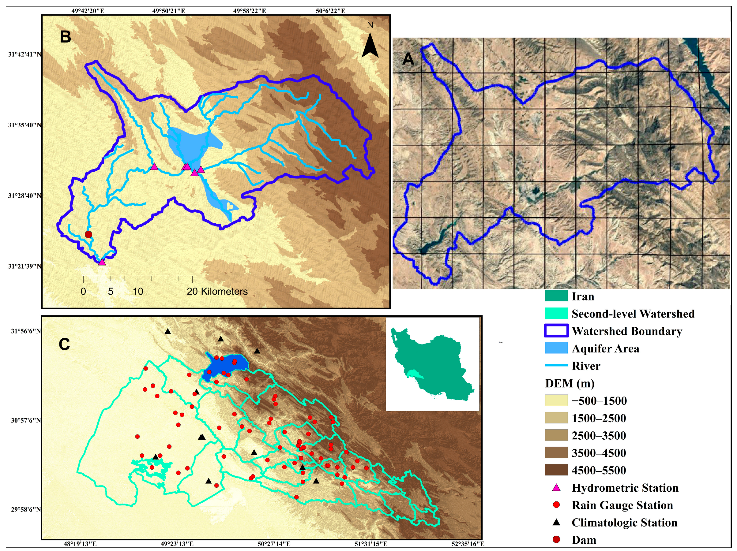
2.1. Study Domain

The Roodzard watershed, with a drainage area of about 900 km² and an altitude ranging between 391.7 m and 3303.3 m, is located in the eastern part of Khuzestan province with the following geographical coordinates: longitude 49°39′ to 50°11′ E and latitude 31°22′ to 31°42′ N (Figure 1). The watershed has different climatic conditions, including a mountainous climate in the highlands (i.e., the eastern parts of the watershed) and a warm climate in the plains areas (i.e., the central parts of the watershed). Based on the Köppen–Geiger climatic index [20], the watershed is classified as BSk (arid, steppe, cold arid) and Cfb (warm temperate, fully humid, warm summer), which describe its arid and semi-arid climate.

The watershed has a high level of vegetational diversity and different land coverage, such as pastures and forests, barren lands, agricultural fields, water bodies, and urban areas. The highland areas of the watershed located on the eastern side are covered by forest (especially oak). Good pasturelands are also located in the upper parts of the watershed and are considered to be nomadic areas. Meanwhile in the lower parts of the watershed, the vegetation density decreases due to geological formations, such as Aghajari and Gachsaran, urbanization, and low precipitation.

From a hydrological point of view, more than 70% of the annual streamflow in the watershed is generated during the winter and spring seasons. The Mashin hydrometric station, where the outgoing streamflow of the watershed is recorded, is located in the southwestern part of the watershed. It should be noted that an embankment storage dam with a reservoir capacity of 260 MCM (million cubic meters) was built upstream of the Mashin station in 2010.

The watershed’s groundwater resources include an alluvial aquifer in the center with an approximate area of 50.88 km², along with karst water resources (in the Asmari formation) in the highlands. Karst resources overlook the aquifer and feed it continuously.

2.2. Data Sources

The datasets utilized in the current research include ground and global gridded information (reanalyses and remotely sensed products). According to the findings acquired by [21], the data preprocessing was performed on a 5 × 5 km² computational domain covering the entire watershed during 2001–2015 with a monthly time step due to the temporal overlap between ground and large-scale information.

2.2.1. Ground-Based Data

The meteorological data recorded by Iran’s Meteorological Organization and Ministry of Energy include relative humidity, sunshine hours, wind speed, and air temperature with a monthly temporal resolution. The ground-based LST has also been used in order to evaluate the LST outcomes. The precipitation data recorded by the Ministry of Energy’s rain gauge stations and their geographical characteristics have been used to generate the spatial distribution of the precipitation.

The hydrological data applied in the calibration of climatological and groundwater balance models include the monthly observed streamflow at the watershed’s outlet (the Mashin station) between 2001 and 2015, along with the piezometric-level data for 2006–2015 based on daily information. The lumped piezometric-level values for the aquifer area have been calculated using the Thiessen polygon method. It should be noted that the dam effect has been removed from the dataset using the historical information of upstream and downstream hydrometric stations.

2.2.2. Gridded Data

The IGBP-DIS (International Geosphere–Biosphere Programme Data and Information System) product, which encompasses global information of soil distribution and features with a spatial resolution of 8 km [22], has been used to derive the soil field capacity and wilting point. The TRMM 3B43 (V7) product has been employed along with monthly in situ precipitation values in order to generate monthly distributions of precipitation over the computational domain. The optimized moving least square (MLS) [23,24] method has been selected due to its acceptable performance in areas with missing data to combine the ground and satellite precipitation data. The method uses weighting functions and moving calculation ranges to weight local values based on their behavior and importance. Estimations are based on weighted least squares. In this method, a weight value is assigned to each point proportionate to its distance; the smaller this distance, the greater its impact on the estimation value. The points that are inside the calculation range participate in the estimation, and the other points have no effect. The MLS method uses DEM properties (latitude, longitude, and elevation) to calculate the distance. In this study, as mentioned before, in order to increase the accuracy of spatial estimation, TRMM 3B43 precipitation has been used as supplementary information alongside the DEM properties to calculate the distance value [25]. Similar to the precipitation, the extraction of the wind speed values over the watershed has been implemented by combining the global gridded and station data. For this purpose, monthly ERA5-Land wind speed data with a spatial resolution of 10 km have been used. The other remotely sensed information required for the modeling is NDVI (MODI13A1), LAI (MODI15A2H), ALBEDO (MCD43A3), and LULC map (MCD12Q1) from the MODIS sensor.

To evaluate the performance of the proposed model, the LST retrievals of MODIS (MOD11C3) and ERA5-Land have been used. MOD11C3 was developed based on seven MODIS TIR bands (bands 20, 22, 23, 29, and 31 to 33) with a spatial resolution of 5 km and a monthly temporal resolution. Likewise, the monthly ERA5-Land surface temperature data were provided through the results of the H-TESSEL (Tiled ECMWF Scheme for Surface Exchanges over Land incorporating Land Surface Hydrology) land surface model and data assimilation techniques with a spatial resolution of 10 km [26]. The properties of the utilized large-scale datasets are listed in

Table 1. The utilized gridded products, along with their temporal and spatial resolutions.

Data	Temporal Resolution	Spatial Resolution	Variable	Web Address
IGBP-DIS	Annual	8 km	Wilting point	https://daac.ornl.gov (accessed on 11 November 2000)
			Field capacity
TRMM	Monthly	25 km	Precipitation (3B43 V7)	https://disc.gsfc.nasa.gov (accessed on 1 January 1999)
ERA5-Land	Monthly	10 km	Wind speed	https://cds.climate.copernicus.eu (accessed on 1 January 1950)
ERA5-Land	Monthly	10 km	LST	https://cds.climate.copernicus.eu (accessed on 1 January 1950)
MODIS	Monthly	1 km	NDVI (MOD13A1)	https://lpdaac.usgs.gov (accessed on 18 February 2000)
MODIS	8-Day	0.5 km	LAI (MOD15A2H)	https://lpdaac.usgs.gov (accessed on 18 February 2000)
MODIS	Monthly	5 km	LST (MOD11C3)	https://lpdaac.usgs.gov (accessed on 1 February 2000)
MODIS	Daily	1 km	ALBEDO (MCD43A3)	https://lpdaac.usgs.gov (accessed on 24 February 2000)
MODIS	Annual	0.5 km	LULC (MCD12Q1)	https://lpdaac.usgs.gov (accessed on 1 January 2001)

.

3. Modeling Procedure

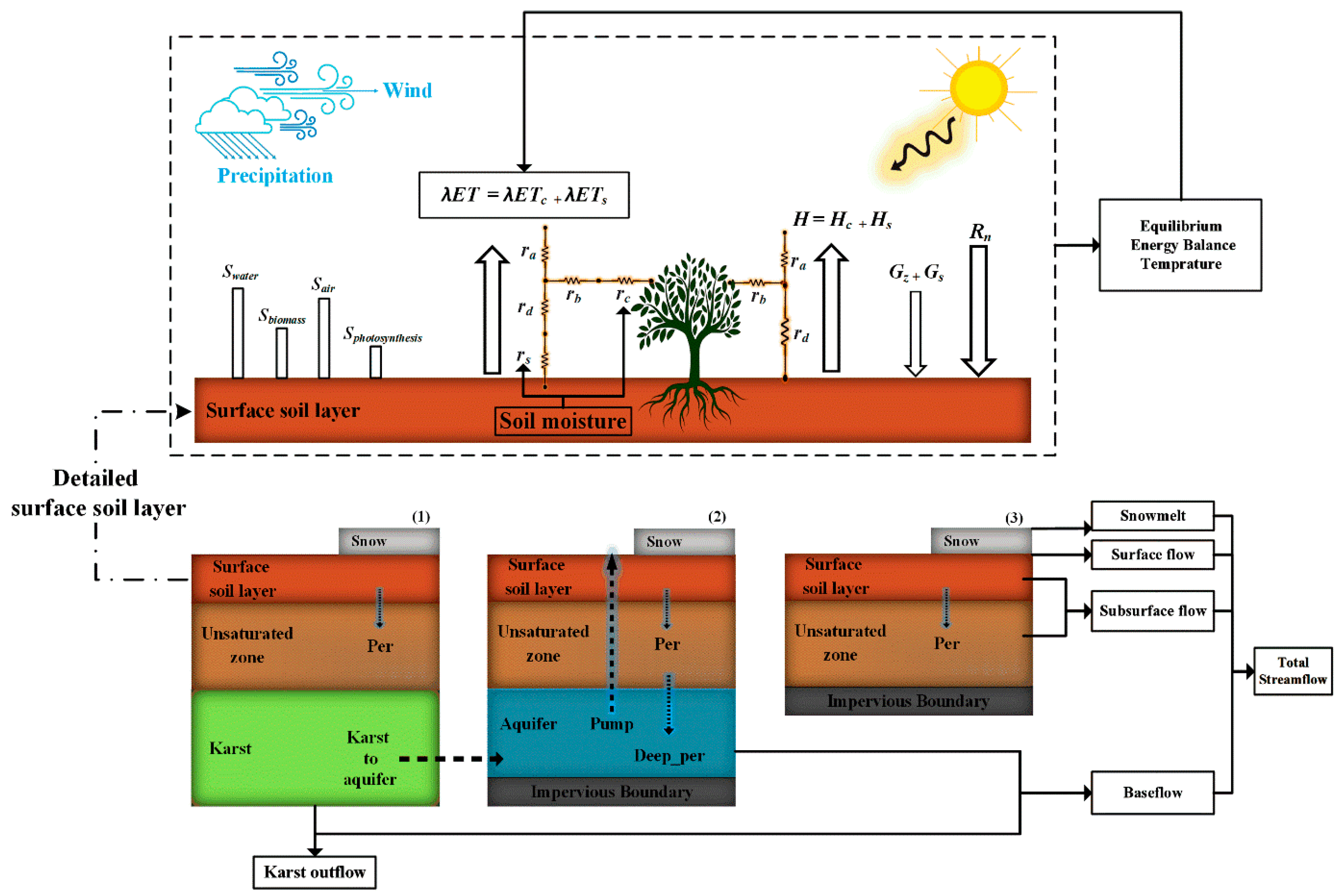
3.1. MCSD-EWB Model Description

MCSD-EWB (Monthly Continuous Semi Distributed Energy Water Balance) is a monthly hydrological model based on water and energy budgeting with a semi-distributed structure. MCSD-EWB has been developed by simultaneously coupling the full surface energy balance (FSEB) and continuous water balance models. The water–energy balance equations system has been solved as a function of the equilibrium energy balance temperature (EEBT) in which the energy balance is closed. It should be noted that EEBT is considered the representative of the LST variable in this study. The full surface energy and water balance models have been developed based on a spatial distributed approach, while the groundwater balance model is based on a lumped modeling approach.

The notable point in the MCSD-EWB model is the simultaneous interconnections of water and energy balances through EEBT, which is achieved from solving the energy balance equation by the Newton–Raphson method. The actual ET estimated based on surface soil moisture and EEBT is applied to the water balance model as a forcing variable and supplied by several surface water resources, including the available water content, the moisture of the subsurface soil layer, and the groundwater. These resources are exploited in a particular order as stated below.

First, the available water resources, including rainfall and upper layer soil moisture, are exploited to provide the actual ET. In this condition, if the resources supply the actual ET, the remnant water is considered to be the moisture of the surface layer. Otherwise, the subsurface soil moisture is exploited to supply the deficit. Thus, the surface soil water will be zero.

Second, if the ET is not supplied by the subsurface soil moisture, the deficit should be satisfied by a withdrawal from the aquifer. In this regard, an extra amount of water, in addition to the water deficit, is pumped to the surface soil layer. The surface and subsurface flows and percolation will be zero after supplying the ET if the surface soil moisture calculated in the previous step is smaller than its saturation capacity; otherwise, they will be calculated as a fraction of the excess moisture above the surface soil storage capacity. As a result, the surface soil moisture is updated in this step by subtracting the surface soil moisture that remains after the ET supply from the sum of surface and subsurface flows and percolation.

Finally, the updated surface soil moisture is utilized to estimate the EEBT and actual ET through soil and canopy surface resistances for the next time step. Additionally, the soil moisture is updated as a result of the ET being forced to be supplied by water resources in the watershed. The coupling process is continued throughout the study period, and to find the optimized parameters, the model is calibrated based on the observed streamflow and groundwater level.

The schematic connections and the components of the model are shown in Figure 2. According to the proposed model, Equations (1) and (2) describe the system governing the water and energy balance.

$$S\left(t\right)-S\left(t_0\right)=\underset{t=0}{\overset{t=t}{{\displaystyle \int }}}\left[R_n\left(t\right)-G\left(t\right)-H\left(t\right)-\lambda ET\left(t\right)\right]dt$$

(1)

$$SM\left(t\right)-SM\left(t_0\right)=\underset{t=0}{\overset{t=t}{{\displaystyle \int }}}\left[P\left(t\right)-R\left(t\right)-ET\left(t\right)\right]dt$$

(2)

where S, R_n, H, λET, SM, P, R, ET, t, and t₀ are the heat storage flux, net radiation flux, soil heat flux, sensible heat flux, latent heat flux, soil moisture, precipitation, streamflow, evapotranspiration, current time step, and previous time step, respectively. The dimensions of the water and energy fluxes are mm and W/m², respectively. The latent heat flux is transformed into an equivalent ET in mm by using the latent heat of vaporization and water density terms. In the following sub-sections, the energy and water balance models are described in detail.

In the current study, the ERA5-Land and MODIS surface temperatures have been employed as inputs into the MCSD-EWB model to further investigate the proposed model. These models, known as MCSD-EWB (ERA5-Land) and MCSD-EWB (MODIS), have followed the water balance structure and the ET estimation method used in the MCSD-EWB model; however, there are some differences between them and the developed model about the dataset associated with surface temperature and the calculation of net radiation, sensible heat, soil heat, and heat storages fluxes, shown in

Table 2. A comparison between the structure of the developed model and other models.

Models	Estimation of Energy Balance Components					Estimation of Water Balance Components
	Net radiation Flux	Sensible heat Flux	Soil heat Flux	Latent heat Flux	Heat storage Flux	Precipitation	Soil moisture	Streamflow	Groundwater Level	Snowmelt	Karst hydrology
MCSD-EWB	✓	✓	✓	✓	✓	✓	✓	✓	✓	✓	✓
MCSD-EWB (ERA5-Land)	✕	✕	✕	✓	✕	✓	✓	✓	✓	✓	✓
MCSD-EWB (MODIS)	✕	✕	✕	✓	✕	✓	✓	✓	✓	✓	✓

. In other words, the LST retrieval method is the origin of the difference between the models. In the MCSD-EWB model, the LST is obtained by closing the full energy balance equation; thus, all fluxes, including radiative, turbulent, and storage fluxes, needed to be calculated. Meanwhile, the MCSD-EWB (ERA5-Land) and MCSD-EWB (MODIS) models are driven by LST products of ERA5-Land and MODIS, respectively.

3.1.1. Full Surface Energy Balance Model

According to the full surface energy balance (FSEB) model provided by Equation (1), the available energy partitioning (R_n-G-S) between the turbulent heat fluxes (H + λET) is controlled by the temperature gradient on the land surface. Since the Newton–Raphson method is one of the most popular methods for estimating functions with a zero value [2] and is acceptable for solving energy balance equation under various hydro-climatic conditions, this method has been used to solve the FSEB equation and estimate EEBT (Equation (3)).

$$EEBT\left(x,t\right)=EEBT\left(x,t-1\right)+\frac{f_t\left(EEBT\left(x,t-1\right)\right)}{f_t^{\prime }\left(EEBT\left(x,t-1\right)\right)}$$

(3)

where $f_t\left(EEBT\right)$ and $f_t^{\prime }\left(EEBT\right)$ are the function of energy balance and its derivative with respect to the equilibrium temperature, respectively.

The energy fluxes of the FSEB model, including radiative, turbulent, and storage terms, are explained in

Table 3. Definitions and relationships of energy fluxes in W/m².

No.	Equation	Description	Variables	References
1	$R_n=\left(1-alb\right)R_{s,in}+R_{l,in}-{\epsilon }_s\sigma EEB{T}^4$	Rn is mostly defined as the sum of the radiation components of incoming and outgoing long- and short-wave radiation.	Rs,in = incoming shortwave radiation (W/m2) $R_{l,in}$= incoming longwave radiation (W/m2) alb = surface albedo (dimensionless) εs = surface emissivity (dimensionless) σ = Stefan–Boltzmann constant (5.67 × 10−8 W.m−2k−4) EEBT = Energy Balance Equilibrium Temperature (K)	Rs,in has been estimated using model proposed by [33]. Rl,in and Rl,out have been calculated by Stefan–Boltzmann equation.
2	$G_z=R_n \left[{\mathsf{Г}}_C+\left(1-f_v\right)\left({\mathsf{Г}}_s-{\mathsf{Г}}_C\right)\right]$	G is the conducted heat between the surface and underground soil layer due to the temperature difference.	Gz = soil heat flux at depth z (W/m2) ${\mathsf{Г}}_C$$,{\mathsf{Г}}_s$= is the ratio of soil heat flux to net radiation flux for areas with dense vegetation cover (equal to 0.05) and bare lands (equal to 0.315), respectively fv = the vegetation ratio (for separation of soil and canopy)	[34]
3	$H=H_c+H_s=$ $(1-f_v)\left(\frac{{\rho }_a{C}_p}{r_{a,s}}\right)\left(EEBT-T_a\right)+f_v\left(\frac{{\rho }_a{C}_p}{r_{a,c}}\right)\left(EEBT-T_a\right)$	H is the heat energy exchanged when there is a temperature gradient between the land surface and atmosphere layer near the surface.	Hc, Hs = canopy and soil sensible heat flux (W/m2), respectively ρa = air density at constant pressure (Kg.m−3) Cp = the specific heat capacity of air at constant pressure (1004 J.kg−1. K−1) Ta = air temperature (K) ra,s, ra,c = aerodynamic resistances of soil and vegetation (s.m−1), respectively	ra,s and ra,c have been estimated using the relationship suggested by [35] and similarity theory (MOST) by [36]
4	$\lambda ET=\lambda E{T}_c+\lambda E{T}_s=f_v\left(\frac{{\rho }_a{C}_p}{\gamma \left(r_{a,c}+r_c\right)}\right)\left(e_s^{\ast }\left(EEBT\right)-e_a\right)+\left(1-f_v\right)\left(\frac{{\rho }_a{C}_p}{\gamma \left(r_{a,s}+r_s\right)}\right)\left(e_s^{\ast }\left(EEBT\right)-e_a\right)$	λET is the energy required to change the water phase from liquid to vapor.	$\lambda E{T}_c$$,\lambda E{T}_s$ = latent heat fluxes for vegetation and soil (W/m2), respectively γ = psychometric constant (kPa °C−1) λ = the latent heat of vaporization (KJ.kg−1.C−1) rs, rc = surface resistances of soil and vegetation, in that order (s.m−1) $e_s^{\ast }$ = saturated vapor pressure in equilibrium temperature (kPa) ea = actual vapor pressure (kPa)	rs and rc have been computed using relations proposed by [28].
5	$S_{air}={{\displaystyle \int }}_0^{z_m}{\rho }_a{c}_p\frac{d{T}_a}{dt}dz$	${\mathit{S}}_{\mathit{a}\mathit{i}\mathit{r}}$ is defined as the stored energy in the air from the surface to measurement height of air temperature.	$z_m$ = The measurement height of the air temperature to the surface level (m) $\frac{d{T}_a}{dt}$ = Air temperature gradient at the desired height with respect to time	[37]
6	$S_{water}={{\displaystyle \int }}_0^{z_m}\lambda {\rho }_a\frac{d{q}_s}{dt}dz$	${\mathit{S}}_{\mathit{w}\mathit{a}\mathit{t}\mathit{e}\mathit{r}}$ indicates the latent heat storage in the air and is computed for the area between the ground surface and the measurement height.	$q_s$= Specific humidity (dimensionless)	[38]
7	$S_{soil}={\displaystyle \sum _0^{z_m}}{c}_s\frac{dEEBT}{dt}d{z}_s$	${\mathit{S}}_{\mathit{s}\mathit{o}\mathit{i}\mathit{l}}$ indicates the energy stored in the soil over time.	$d{z}_s$ = Thicknesses of various soil layers (m) $dEEBT$ = Temperature gradient in different soil layers (K) $c_s$ = Volumetric heat capacity of the soil $(\mathrm{MJ}.{\mathrm{m}}^{-3}{\mathrm{K}}^{-1}$) [39]	[40,41]
8	$S_{biomass}={{\displaystyle \int }}_0^{z_m}{m}_b{c}_b\frac{d{T}_c}{dt}$	${\mathit{S}}_{\mathit{b}\mathit{i}\mathit{o}\mathit{m}\mathit{a}\mathit{s}\mathit{s}}$ indicates the energy stored in the canopy over time.	$m_b$$=\mathrm{Biomass}\mathrm{per}\mathrm{unit}\mathrm{area}(\mathrm{kg}.{\mathrm{m}}^{-2}$) $c_b$= Specific heat capacity of biomass (J.Kg−1.K−1) $\frac{d{T}_c}{dt}$ = Canopy temperature gradient with respect to time (K)	[37]
9	$S_{photosynthesis}=$$11.2\times m_b$	During the heat storage due to photosynthesis process, the carbon dioxide flux is transformed into energy flux in such a way that 11.2 watts of energy is generated in each square meter, corresponding to the absorption of each gram of carbon dioxide.	-	[42]

. According to the table, H and λET are estimated via the bulk heat transfer theory, and due to the sparsity of vegetation over the study region, the patch approach [27] has been utilized to distinguish turbulent fluxes for the canopy and bare soil components. The aerodynamic resistances of the sensible and latent heat fluxes have been determined by Equation (4) for the soil and canopy. In addition, the surface resistances for soil and vegetation have been computed using the relationships proposed by [28], respectively, as shown below:

$$r_a=\frac{[ln\left(\frac{z_m-d}{z_{om}}\right)-{\psi }_m(\frac{z_m-d}{L})]ln[\left(\frac{z_h-d}{z_{oh}}\right)-{\psi }_h(\frac{z_h-d}{L})]}{k^2{u}_z}$$

(4)

$$r_s=exp\left(8.206-4.255\left(\raisebox{1ex}{$w_z$}\!\left/ \!\raisebox{-1ex}{$w_{sat}$}\right.\right)\right)$$

(5)

$$r_c=\frac{r_{s,min}}{LAI}{F}_1^{-1}{F}_2^{-1}{F}_3^{-1}{F}_4^{-1}$$

(6)

where z_m and z_h are the heights for measuring wind speed and humidity (m), respectively, d is the displacement height of the zero plate (m), z_om and z_oh denote the length of the roughness governing the momentum and heat/steam transfer (m), respectively, k is the Karman constant (equals 0.41), u_z is the wind speed at height z (m/s), ψ_m and ψ_h are the dimensionless correction functions for momentum and heat transfer in stable and unstable atmospheric conditions, respectively, L is the Monin–Obukhov length (m), w_z is the volumetric soil water content at depth z (m³/m³), w_sat is the saturated soil water content (m³/m³), LAI is the leaf area index (dimensionless), r_s,min indicates the resistance of vegetation against transpiration under ideal conditions (i.e., without soil moisture tension, sufficient light, etc.) (s/m), and parameters F₁, F₂, F₃, and F₄ are environmental stresses (dimensionless). The stress factors are measures of the effects of active photosynthesis radiation, water stress, deficiency in atmospheric vapor pressure, and air temperature on surface resistance, respectively, and have been calculated using Equations (7)–(10), which were proposed by [14,28]:

$$F_1=\frac{f+r_{c,min}/r_{c,max}}{1+f}, f=0.55\frac{R_{s,in}}{R_{s.min,L}}\frac{2}{LAI}$$

(7)

$$F_2=\left\{\begin{array}{c}1 if w_{cr}<w_z\\ \frac{w_z-w_{wilt}}{w_{cr}-w_{wilt}} if w_{wilt}<w_z<w_{cr}\\ 0 if w_z<w_{wilt}\end{array}\right.$$

(8)

$$F_3=1-g\left(e_s^{*}\left(T_s\right)-e_a\right)$$

(9)

$$F_4=1-0.0016{\left(298-T_a\right)}^2$$

(10)

where r_c,min and r_c,max are the minimum and maximum values of canopy resistance, respectively (s/m), which are considered equal to 200 [29] and 5000 [30], respectively; R_s,min,L is a limit value of incident radiation (W/m²); w_cr is the field capacity (m³/m³) close to 0.75 w_sat [31]; W_wilt is the soil moisture at the wilting point (m³/m³); g is an experimental parameter that depends on the plant type, mostly considered as equal to 0.025 (h/pa); and T_a is the mean air temperature (K) at the reference height.

By considering the feasibility of energy accumulation within the soil–vegetation–atmosphere system over a month, the heat storage term has been calculated as the sum of the sensible heat storage (S_air), latent heat storage (S_water), biomass heat storage (S_biomass), photosynthesis heat storage (S_{photosynthesis}), and soil heat storage (S_soil) in W/m², as shown in Table 3. It should be noted that the Carnegie–Ames–Stanford approach (CASA) model [32], which is based on absorbed photosynthetic active radiation (APAR) and light use efficiency (LUE), has been utilized to estimate the biomass production (i.e., m_b, shown in Table 3, row 8).

3.1.2. Water Balance Model

The employed climatological water balance model is based on the conceptual structure proposed by [17] and improved by adding snowpack (snow accumulation and melting). In the model suggested by [17], the soil layer is simulated in two surface and subsurface (unsaturated) layers with different soil moisture capacities. The upper soil layer simulates the surface and subsurface flows and water percolation to the sublayer, while the unsaturated layer between the surface and the saturated (alluvial aquifer) layers simulates the recharge to the aquifer and subsurface flow of the non-saturated layer. Since this model is recommended for dry arid and dry semiarid areas in which snow hydrology is not taken into account, the snow module from the conceptual model suggested by [43] has been used to enhance the model’s behavior and compatibility with the watershed’s climate condition. According to the snow module, snow and rain have been differentiated using the temperature threshold method (two parameters to separate snow and rain). In addition, the snowmelt, which is added to the watershed’s streamflow, has been calculated using the melting coefficient.

Given the presence of an alluvial aquifer in the watershed, a conceptual model of groundwater balance has been used to simulate the fluctuations of groundwater level and groundwater–surface water interactions. The conceptual model proposed by [18] provides an appropriate structure to connect with the aforementioned two-layer water balance model. The groundwater model’s inputs are the deep penetration from the unsaturated layer and areas overlooking the aquifer, and the outputs include the baseflow and amount of withdrawn water (Equation (11)).

$$R\mathsf{\Delta }x\mathsf{\Delta }y-Q=S\mathsf{\Delta }x\mathsf{\Delta }y\frac{dh}{dt}$$

(11)

where R is the aquifer recharge ($\mathrm{m}/\mathrm{s}$), Q is the total groundwater discharge (${\mathrm{m}}^3/\mathrm{s}$) which is calculated using $T\mathsf{\Delta }y\frac{\mathsf{\Delta }h}{0.5\mathsf{\Delta }x}$ (T = Transmissivity (${\mathrm{m}}^2/\mathrm{s}$) and Δh = the difference between groundwater level and the elevation of the baseflow outlet ($\mathrm{m}$)), S is the storage coefficient (dimensionless), dh is the change in groundwater level ($\mathrm{m}$) over time step dt ($\mathrm{s}$), and $\mathsf{\Delta }x$ and $\mathsf{\Delta }y$ are, respectively, the length and width of the aquifer storage cell ($\mathrm{m}$). The hydraulic gradient is calculated between the center of the aquifer, from which the groundwater level is measured by means of a borehole, and the groundwater discharge point, where the river passes through the aquifer at its lowest altitude. Since the model has a lumped structure, the hydraulic gradient is calculated in the x direction. In addition, the baseflow is assumed to occur only when the groundwater level exceeds $h_{discharge\_point}$, which is calibrated during the optimization process.

One remarkable feature of the groundwater model is its specific approach to the contribution of the unsaturated layer in feeding the groundwater reservoir (percolation), which is implemented using the Weibull distribution function while taking into account the effect of various time steps on the penetration procedure (Equation (12)). The Weibull distribution function represents exponentially decreasing and increasing skewed distributions, and this is why it has a stronger justification than other functions for reflecting moisture transfer from the surface and non-saturated layers into the saturated zone.

$$f\left(t_e; q, k\right)=\left\{\begin{array}{c}\frac{k}{q}\times {\left(\frac{t_e}{q}\right)}^{k-1}\times exp\left(-{\left(\raisebox{1ex}{$t_e$}\!\left/ \!\raisebox{-1ex}{$q$}\right.\right)}^k\right) t_e\ge 0\\ 0 t_e<0\end{array}\right.$$

(12)

where $t_e$ represents an effective month on deep penetration (the penetration in each time step depends on that same step in addition to some previous ones), k is the shape factor (controlling the density of the distribution function around the peak), and q is the scale factor (controlling the location of the peak in the distribution function), with their respective values being determined during the optimization process.

In addition to the alluvial aquifer, there are karstic areas in the Asmari formation in the eastern parts of the watershed. In this research, a linear storage reservoir has been utilized to simulate the karst water balance and its interactions with the aquifer and soil layers. The reservoir input is a portion of rain in these regions, and the output includes the evaporation, baseflow, outflow from the karstic area to the outside of the watershed, and the flow entering the aquifer.

Finally, the total streamflow consists of the baseflow, surface and subsurface (each of the two separate soil layers) flows, and snowmelt runoff (Equation (13)). The sum of the generated streamflow values over the computational cells is then compared with the observed values at the watershed outlet.

$$\begin{gathered} Q_{total}\left(t\right)=Q_{Surface}\left(t\right)+Q_{Usub}\left(t\right)+Q_{Lsub}\left(t\right)+Q_{baseflow}\left(t\right) \\ +Kars{t}_{baseflow}\left(t\right)+SNM\left(t\right) \end{gathered}$$

(13)

where t shows the time (month), $Q_{total}\left(t\right)$ is the total streamflow (mm$/{\mathrm{km}}^2$), $Q_{Surface}\left(t\right)$ is the surface flow (mm$/{\mathrm{km}}^2$), $Q_{Usub}\left(t\right)$ is the upper layer’s subsurface flow (mm$/{\mathrm{km}}^2$), $Q_{Lsub}\left(t\right)$ is the lower layer’s subsurface flow (mm$/{\mathrm{km}}^2$), $Q_{baseflow}\left(t\right)$ is the baseflow from groundwater table (mm$/{\mathrm{km}}^2$), $Kars{t}_{baseflow}\left(t\right)$ is the baseflow from karst storage (mm$/{\mathrm{km}}^2$), and $SNM\left(t\right)$ is the snow melt (or meltwater; mm$/{\mathrm{km}}^2$).

3.2. Statistical Performance Metrics

The classic approach to calibrating the parameters for hydrological models is founded on maximizing or minimizing an objective function by comparing the observed and computed streamflow values at hydrometric stations [44]. In the current research, this optimization procedure has been conducted via a combined objective function obtained by multiplying the sum of the absolute error between the simulated and observed streamflow and groundwater levels (Equation (14)):

$$Objective Function={\displaystyle \sum }_{i=1}^n\left|Q_i^{obs}-Q_i^{sim}\right|\times {\displaystyle \sum }_{i=1}^n\left|H_i^{obs}-H_i^{sim}\right|$$

(14)

where Q_i^obs and Q_i^sim are the observed and simulated streamflow, respectively, H_i^obs and H_i^sim are the observed and simulated aquifer levels, respectively, and n is the number of data points. In addition, the shuffled complex evolution (SCE.UA) algorithm from [45] has been utilized to optimize the model’s parameters, as depicted in

Table 4. The model parameters and their ranges.

Name	Unit	bl	bu	Description
Tsnow	°C	−7	−2	Snow threshold temperature
Train	°C	2	8	Rainfall threshold temperature
Ks	-	0.2	0.8	Snowmelt coefficient
LSM	mm	50	120	Lower-layer initial soil moisture
LSMmax	mm	80	200	Lower-layer saturated soil moisture
alpha	-	0.25	0.85	Ratio of the return flow
K1	-	0	0.3	Surface flow coefficient
K2	-	0.1	0.6	Upper-layer subsurface flow coefficient
K3	-	0	0.5	Lower-layer subsurface flow coefficient
K4	-	0.1	0.7	Deep percolation coefficient
K5	m/day	0	20	Hydraulic conductivity coefficient
zp	-	0.1	0.8	Soil porosity
$h_{discharge\_point}$	m	640	700	Groundwater level threshold
q	-	1	6	Scale parameter of the Weibull distribution
k	-	2	8	Shape parameter of the Weibull distribution
n	-	1	9	Maximum number of time steps taken for soil drainage to reach the groundwater
S	-	0	1	Storage coefficient of the aquifer
h0	m	722	726	Initial groundwater level
Karstp	-	0	0.5	Karst storage precipitation ratio
KarstET	-	0	0.3	Karst storage evaporation ratio
Karstbsf	-	0	0.5	Karst storage baseflow ratio
Karstdis	-	0	0.2	Karst storage discharge ratio
Karstwsh	-	0	0.5	Karst storage into the basin (baseflow + Recharge) ratio

, and the calibration and validation periods have been separated randomly.

The main modeling results, including land surface temperature, streamflow, and aquifer level, have been evaluated via the Kling–Gupta efficiency (KGE) and Nash–Sutcliffe efficiency (NSE) measures and a dissimilarity measure of the root mean square error (RMSE), which are presented as follows:

$$KGE=1-\sqrt{{\left(R-1\right)}^2+{(\frac{{\sigma }_{sim}}{{\sigma }_{obs}}-1)}^2+{(\frac{\overline{X_{sim }}}{\overline{X_{obs }}}-1)}^2 }$$

(15)

$$RMSE=\sqrt{\frac{{{\displaystyle \sum }}_{i=1}^N{\left(X_i^{obs}-X_i^{sim}\right)}^2}{N}}$$

(16)

$$NSE=1-\frac{{{\displaystyle \sum }}_{i=1}^N{\left(X_i^{obs}-X_i^{sim}\right)}^2}{{{\displaystyle \sum }}_{i=1}^N{\left(X_i^{obs}-\overline{X_{obs}}\right)}^2}$$

(17)

$$R^2=\frac{cov\left(X_i^{\mathrm{obs}}, X_i^{\mathrm{sim}}\right)}{\sqrt{Var\left(X_i^{\mathrm{obs}}\right)\times Var\left(X_i^{\mathrm{sim}}\right)}}$$

(18)

where X is the variable of interest (e.g., streamflow, aquifer level, and LST), N is the number of data points, σ is the standard deviation of X, R is the correlation coefficient, $\overline{X}$, Var, and cov are the average, variance, and covariance of X, respectively, and Obs and sim indicate the observed and simulated quantities, respectively. The spatial distributions of ET and LST simulated by the MCSD-EWB, MCSD-EWB (ERA5-Land), and MCSD-EWB (MODIS) models have been compared with the measured values using the MAE statistic (Equation (19)):

$$MAE=\frac{{{\displaystyle \sum }}_{i=1}^N{M}_i^{obs}-M_i^{sim}}{N}$$

(19)

where M indicates the ET and LST variables.

4. Results and Discussion

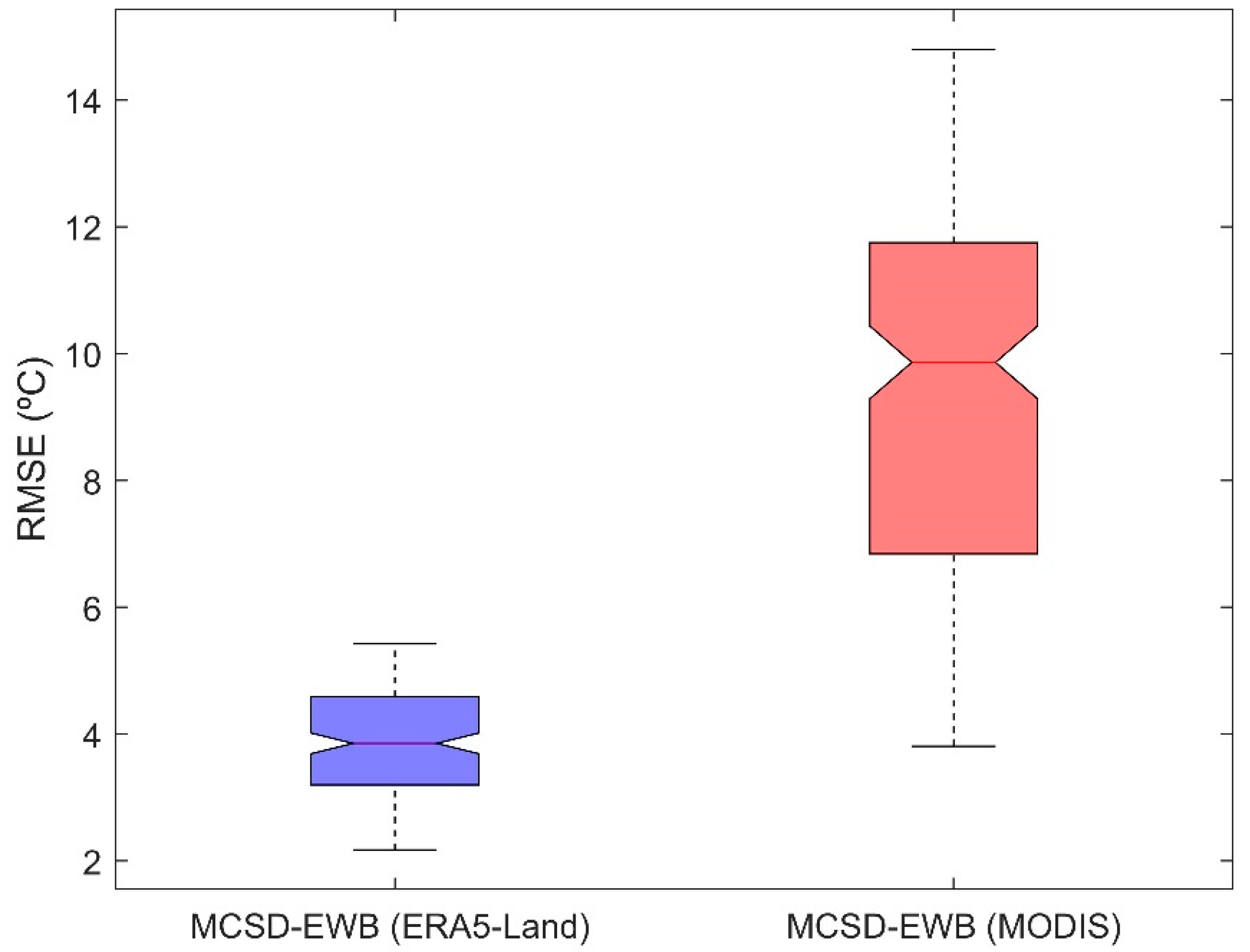
4.1. Evaluation of LST results

4.1.1. Statistical Performance Criteria

Table 5. NSE, RMSE, and KGE metrics in simulating LST by MCSD-EWB, MCSD-EWB (ERA5-Land), and MCSD-EWB (MODIS) models compared to the ground-based LST provided by eight metrological stations.

Station	MCSD-EWB			MCSD-EWB (MODIS)			MCSD-EWB (ERA5-Land)
	KGE	RMSE	NSE	KGE	RMSE	NSE	KGE	RMSE	NSE
Bandar-e-Mahshahr	0.72	4.99	0.5	−0.34	20.54	−7.42	0.13	12.62	−2.17
Behbahan	0.73	4.04	0.74	−0.78	23.29	−7.65	0.06	12.17	−1.36
Dogonbad	0.6	5.89	0.36	−0.86	20.8	−6.92	0.13	9.56	−0.67
Hendijan	0.77	4.31	0.66	−0.59	24.16	−9.68	0.17	12.25	−1.74
Izeh	0.34	7.2	−0.01	−1.46	24.13	−10.4	0.05	9.17	−0.64
Masjed-Soleyman	0.45	7.17	0.21	−0.6	23.6	−7.53	0.24	10.79	−0.78
Omidieh	0.79	4.07	0.69	−0.55	23.99	−9.55	0.2	11.48	−1.41
Ramhormoz	0.68	5.48	0.55	−0.35	21.64	−6.08	0.37	9.66	−0.41

shows the NSE, RMSE, and KGE metrics for the LST results of the MCSD-EWB, MCSD-EWB (ERA5-Land), and MCSD-EWB (MODIS) models compared to the ground-observed LST provided by eight meteorological stations: Bandar-e-Mahshahr, Ramhormoz, Omidieh, Masjed-Soleyman, Izeh, Hendijan, Dogonbad, and Behbahan. According to the results, the MCSD-EWB model has the highest NSE values [−0.01 to 0.74], the lowest RMSE values [4.04 to 7.20], and the highest KGE values [0.34 to 0.79], showing the best performance. By considering the NSE, RMSE, and KGE values of [−0.41 to −2.17], [9.17 to 12.62], and [0.06 to 0.37], respectively, the MCSD-EWB (ERA5-Land) model is ranked second. Meanwhile, the MCSD-EWB (MODIS) model, the third-most-accurate model in estimating the LST, has the highest RMSEs ([20.54 to 24.16]), lowest KGEs ([−0.34 to −1.46]), and lowest NSEs ([−6.08 to −10.4]). This is due to the high LST values of MODIS which result from the large proportion of soil within the sensor IFOV.

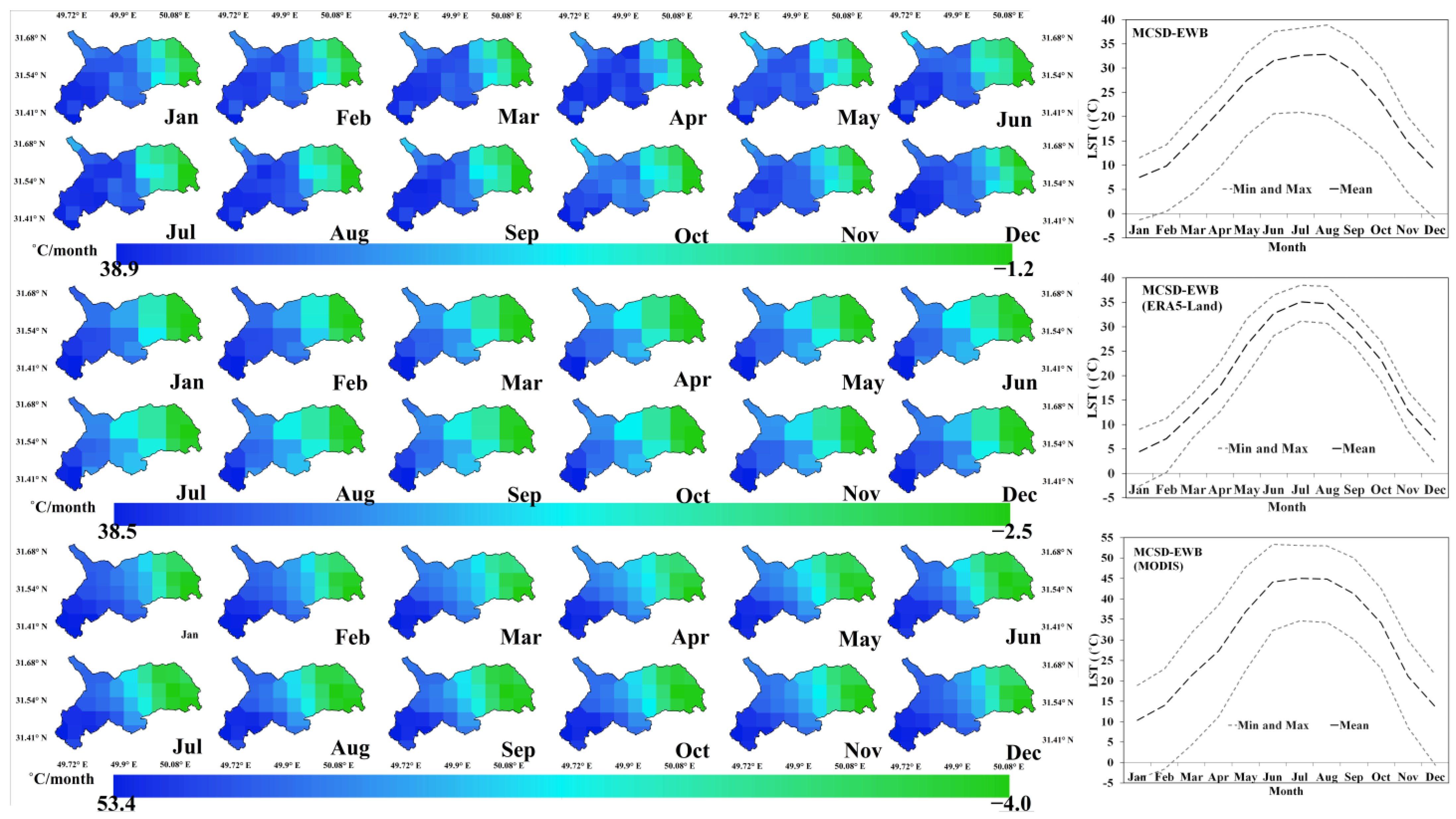
4.1.2. Spatiotemporal Patterns

Figure 3 depicts the spatiotemporal distributions of the long-term monthly average LST simulated by the MCSD-EWB, MCSD-EWB (ERA5-Land), and MCSD-EWB (MODIS) models. According to the figure, the spatial patterns of the models are fairly similar to each other in illustrating the LST variations. The lowest surface temperatures have occurred in the eastern highlands of the watershed, which are covered by snow and dense forest. Due to dense and tall canopies’ ability to access water through their deep roots, a greater amount of ET occurs through transpiration [46]. This results in a decrease in soil heat storage and increase in latent heat flux, resulting in a decrease in surface temperature [47]. In contrast, a gradual increase in land surface temperature can be observed when moving toward the western part of the watershed so that the highest LST values have been obtained in the western and southwestern parts of the watershed because of a significant accumulation of heat within the exposed bare soil and sparse vegetation [48].

Regarding the temporal variations in LST, the lowest and highest temperature values estimated by the MCSD-EWB model are −1.25 °C (in January) and 38.92 °C (in August), respectively. Moreover, the LST values averaged over the watershed vary between 7.48 and 32.83 °C, which occurred in January and August, respectively. On the other hand, the LST values based on the MCSD-EWB (ERA5-Land) model range between −2.56 °C (in January) and 38.52 °C (in July), and the highest and lowest values for the spatially averaged LST are 4.43 °C and 35.09 °C, respectively. The temporal pattern of the LST in the MCSD-EWB (MODIS) model is similar to those of the other two models, in that the lowest and highest temperatures are −4 °C (in January) and 53.37 °C (in June), respectively. According to this model’s results, the mean LST values vary between 10.37 °C (in January) and 45.01 °C (in July). The LST changes in the MCSD-EWB (MODIS) model are broader than those from the other models; however, the dominant temporal trends are similar in all three models.

4.1.3. Performance Assessment Based on EEBT

To reflect the spatial behavior of the EEBT variable in comparison with that of the LST of the MCSD-EWB (ERA5-Land) and MCSD-EWB (MODIS) models, the spatial distributions of the MAE metric for monthly EEBT values and the aforementioned LST results are illustrated in Figure 4. The minimum, average, and maximum values of MAE for the EEBT and LST of the MCSD-EWB (ERA5-Land) and MCSD-EWB (MODIS) models are 1.6, 3.18, and 8.7 °C and 4.51, 8.89, and 13.31 °C, respectively. Thus, the difference between the EEBT and surface temperature of the MCSD-EWB (ERA5-Land) model is less than that between the EEBT and LST of the MCSD-EWB (MODIS) model. This can be attributed to the relatively similar structure of MCSD-EWB and ERA5-Land in retrieving LST, which is an energy-balance-closure-based approach.

According to the spatial distribution of MAE, the largest difference between the EEBT and simulated LST values by the MCSD-EWB (ERA5-Land) model occurred in the eastern part of the watershed. Meanwhile, the largest differences between the EEBT and LST of the MCSD-EWB (MODIS) model are observed in the northeastern, northwestern, and southwestern parts of the watershed.

Figure 5 shows the boxplots of the RMSE metric associated with the monthly EEBT values compared to LST results of the MCSD-EWB (ERA5-Land) and MCSD-EWB (MODIS) models. Accordingly, the minimum, maximum, and median RMSE for the MCSD-EWB (ERA5-Land) and MCSD-EWB (MODIS) models are 2.17, 5.42, and 3.85 °C and 3.80, 14.79, and 9.86 °C, respectively. Similar to the MAE results, the results for the EEBT are in better agreement with the LST of the MCSD-EWB (ERA5-Land) model than with that of the MCSD-EWB (MODIS) model.

In general, the MCSD-EWB model is more accurate in simulating LST than the other models. This can be attributed to the method employed by this model in which the model considers the reciprocal interconnections of water and energy balances and simultaneously solves the equations to calculate the LST.

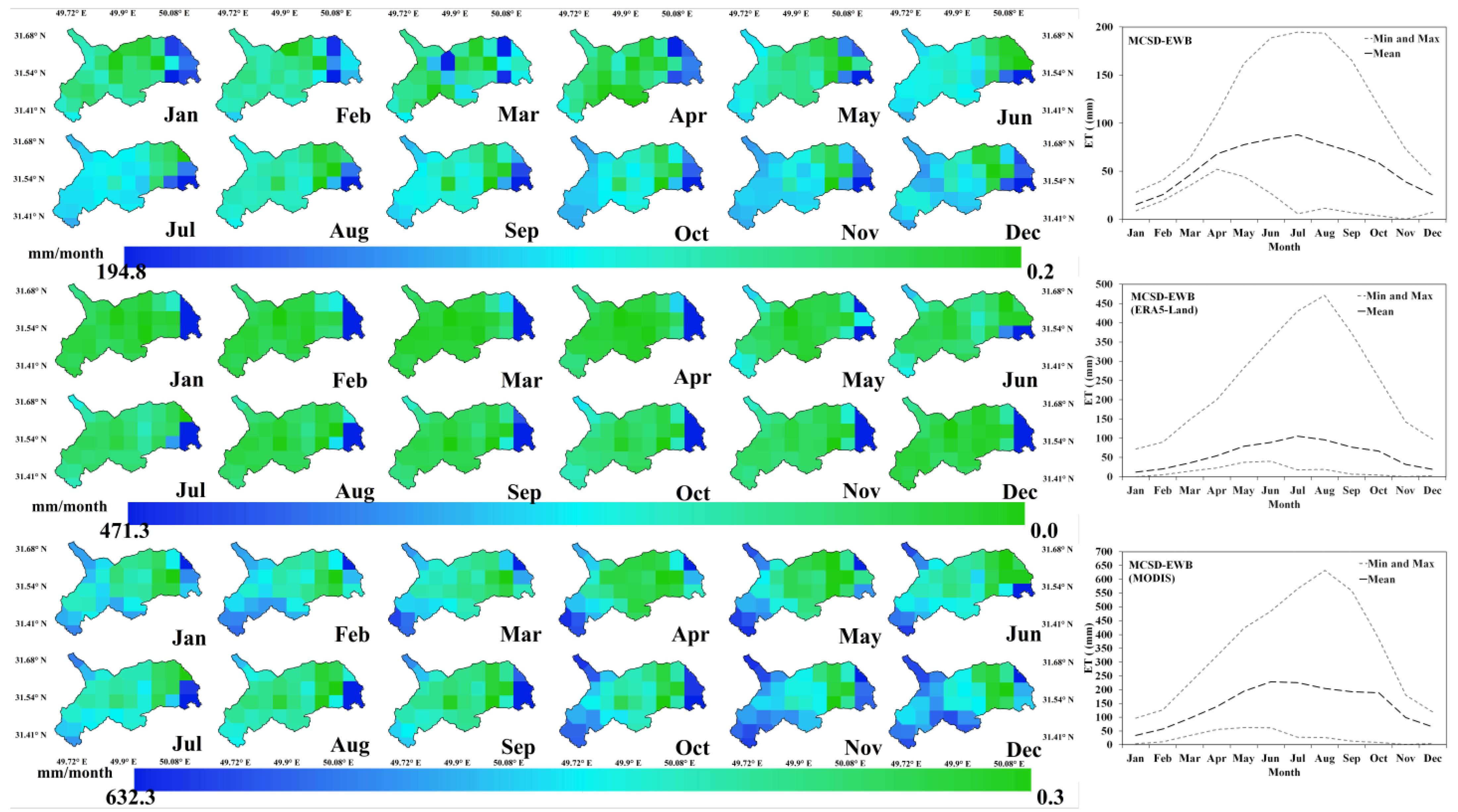
4.2. Evaluation of ET Results

4.2.1. Spatiotemporal Patterns

Figure 6 shows the spatiotemporal distributions for the long-term monthly average of the ET simulated by the MCSD-EWB, MCSD-EWB (ERA5-Land), and MCSD-EWB (MODIS) models. The highest ET values obtained from the MCSD-EWB model have mainly occurred in the eastern parts of the watershed due to the vegetation cover, leading to the increased ET, both physiologically and structurally. In addition, the highlands are exposed to more water sources, such as rainfall and snowmelt, which reduce the water supply constraint for a high ET rate. The southwestern area of the watershed, where the dam is located, also has higher ET values than the surrounding regions because of the high potential of the reservoir to absorb solar radiation and the high atmospheric demand, leading most of the stored energy to be partitioned into evaporation. Similar to the MCSD-EEWB model, the MCSD-EWB (ERA5-Land) model has the highest ET values in the eastern parts of the watershed. In addition, in warm months (April to October), the simulated ET values are larger at the dam location than in the other areas. This model has shown a uniform behavior for the simulated ET, with no significant changes in other parts of the watershed.

The monthly spatial patterns of the ET simulated using the MCSD-EWB (MODIS) model depict different spatiotemporal behaviors. In January, February, and March, the maximum ET values are observed in the northeastern, southeastern, and northwestern parts of the watershed, respectively, while during April and May, these values have occurred in the northeastern and southwestern areas due to the reservoir and dense canopy. These maximum quantities are seen in the southeastern parts of the watershed and then around the dam location in the warm months (i.e., June, July, August, and September).

The spatial trends of the ET for October, November, and December are fairly similar, and the largest ET values have occurred in the eastern, northwestern, southern, and southwestern parts of the watershed. It is worth noting that the significant spatial variations in ET occurred mainly in these months according to the results of the MCSD-EWB (MODIS) model. Unlike the uniform spatial patterns of ET simulated using MCSD-EWB (ERA5-Land), the MCSD-EWB and MCSD-EWB (MODIS) models have shown a non-uniform pattern with noteworthy variations. However, the MCSD-EWB (ERA5-Land) model has shown more similarity to MCSD-EWB than MCSD-EWB (MODIS).

According to the temporal variations in the simulated ET, the results of the MCSD-EWB model vary between 0.22 and 194.79 mm, which occurred in November and July, respectively. Moreover, the largest and lowest values of the averaged ET over the watershed have been yielded as 15.37 mm (in January) and 87.87 mm (in July). The ET values achieved via MCSD-EWB (ERA5-Land) have been bounded between 0.0067 mm (January) and 471.3 mm (August), and the maximum and minimum of the spatially averaged ET are 11.8 mm (January) and 105.21 mm (July). The temporal pattern of the ET estimated by the MCSD-EWB (MODIS) model is similar to that of the other models, with the maximum and minimum values being 0.34 mm (November) and 632.34 mm (August), whereas their monthly mean values are 33.95 mm (January) and 228.62 mm (June), respectively. To close, the temporal patterns of the ET simulated using all models are similar to each other. On average, the maximum and minimum values of the simulated ET have been obtained by the MCSD-EWB (MODIS) and MCSD-EWB models, respectively.

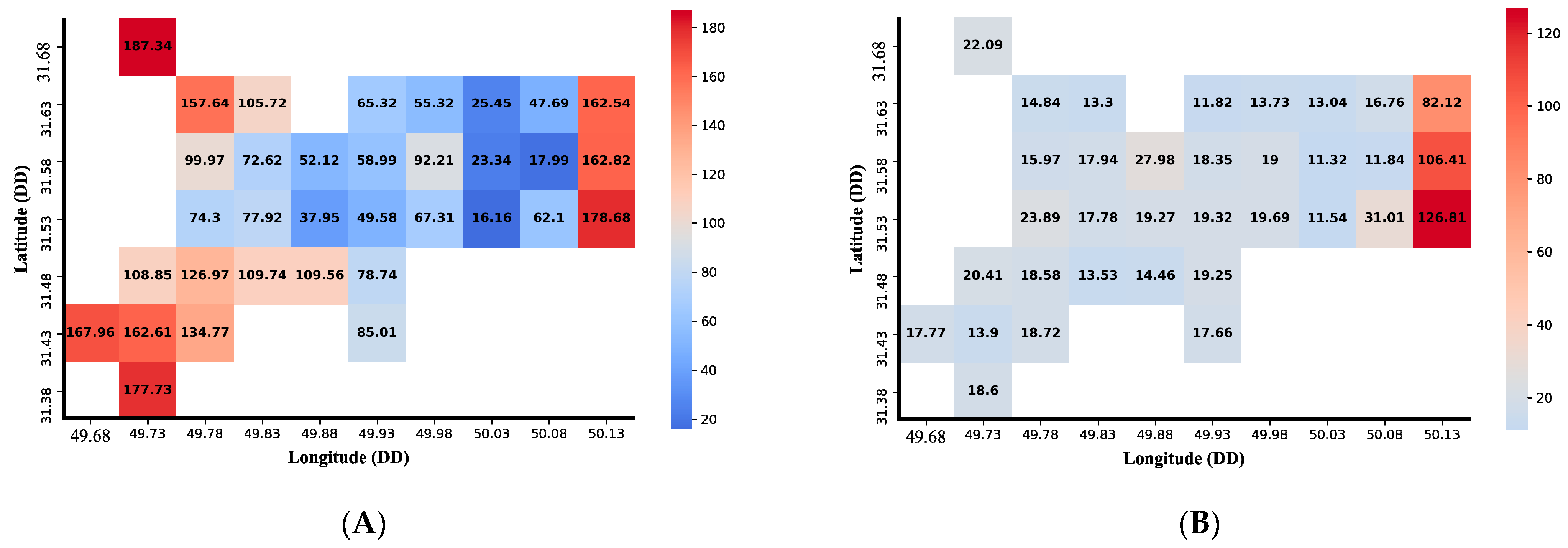
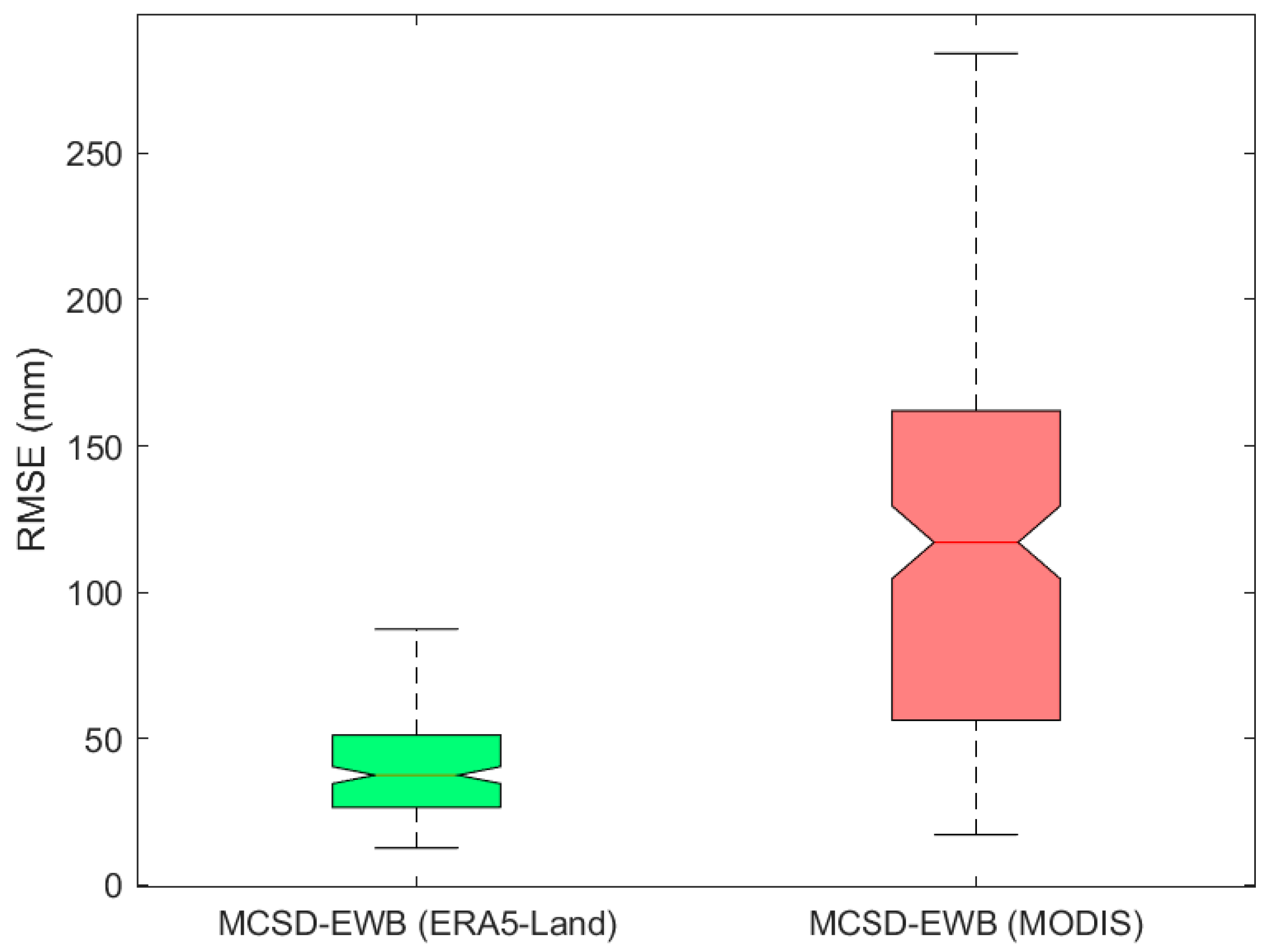
4.2.2. Performance Assessment Based on Modeled ET

Figure 7 shows the spatial distributions of the MAE metric between the monthly ET values of the MCSD-EWB model and the other models (MCSD-EWB (MODIS) and MCSD-EWB (ERA5-Land)). Based on the patterns, the MAE metric between the simulated ET of the MCSD-EWB and MCSD-EWB (MODIS) models has maximum, minimum, and average values equal to 178.68, 16.16, and 94.5 mm, respectively. In addition, these values are 126.81, 11.32, and 25.25 mm for the MAE metric between the ET of the MCSD-EWB and MCSD-EWB (ERA5-Land) models. Therefore, the ET results of MCSD-EWB are more similar to those of MCSD-EWB (ERA5-Land) than MCSD-EWB (MODIS). The largest dissimilarity between MCSD-EWB and MCSD-EWB (ERA5-Land) in simulating the ET is observed in the eastern part of the watershed; however, it occurs in the eastern, northern, and southwestern areas in the case of the MCSD-EWB (MODIS) model.

In addition to the assessment by the MAE measure, the boxplots of the RMSE statistics between the monthly ET values estimated by the MCSD-EWB model and the other models (MCSD-EWB (MODIS) and MCSD-EWB (ERA5-Land)) are presented in Figure 8. Accordingly, the minimum, maximum, and median values of the metric for the developed model and MCSD-EWB (MODIS) are 17.02, 284.16, and 116.99 mm. These values in the case of MCSD-EWB (ERA5-Land) are 12.49, 87.30, and 37.38 mm. Hence, the results of MCSD-EWB are more compatible with MCSD-EWB (ERA5-Land) than MCSD-EWB (MODIS).

Given that LST is a key factor controlling the ET process, its estimation accuracy significantly affects the determination of accurate ET values. Based on Section 4.1, the LST values of MCSD-EWB (ERA5-Land) and EEBT are in good agreement with in situ measurements, while the LSTs of MCSD-EWB (MODIS) have been overestimated in comparison with two other models. Therefore, it can be concluded that the ET simulated by MCSD-EWB (MODIS) is more unrealistic and less accurate than the MCSD-EWB and MCSD-EWB (ERA5-Land) models.

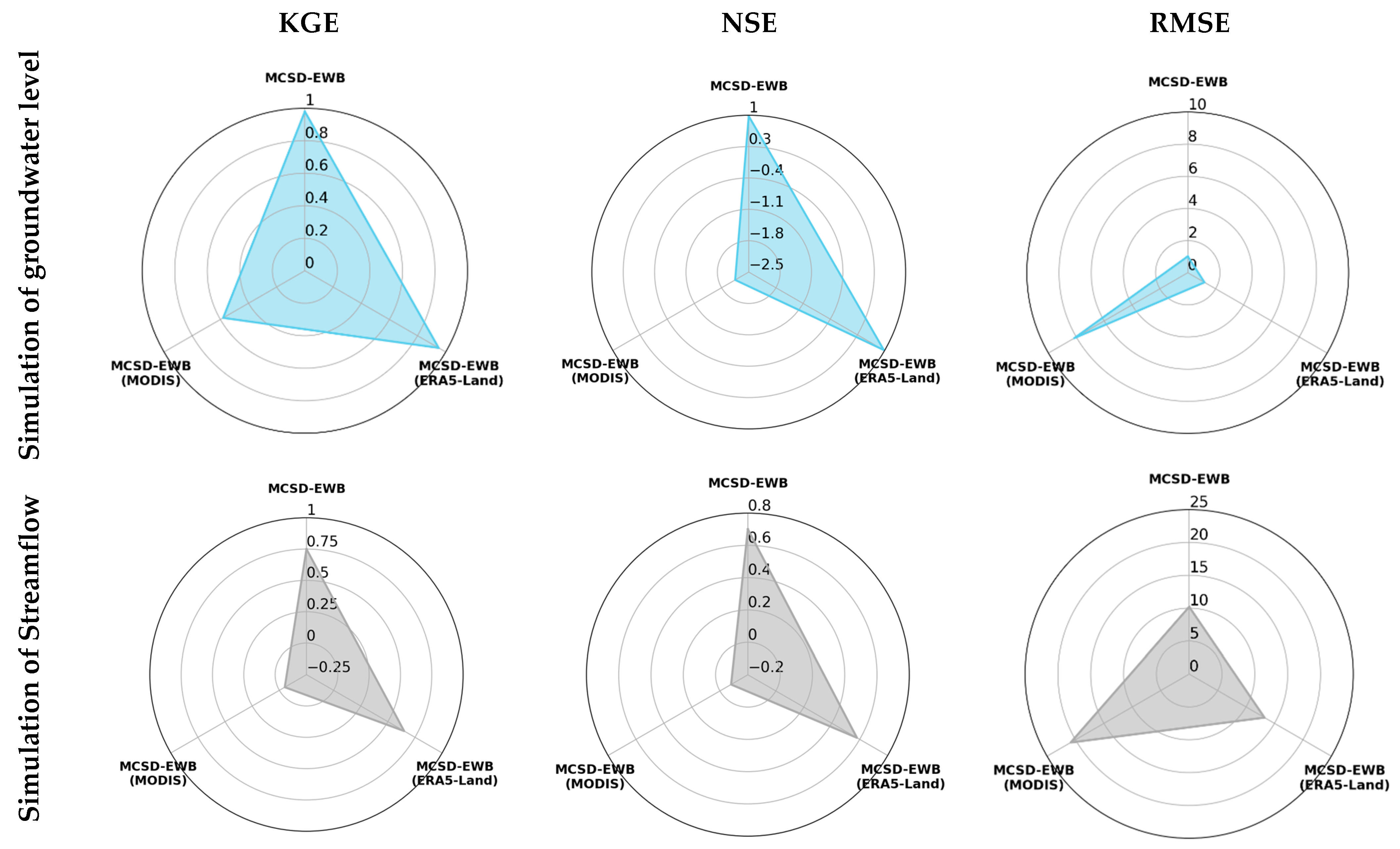
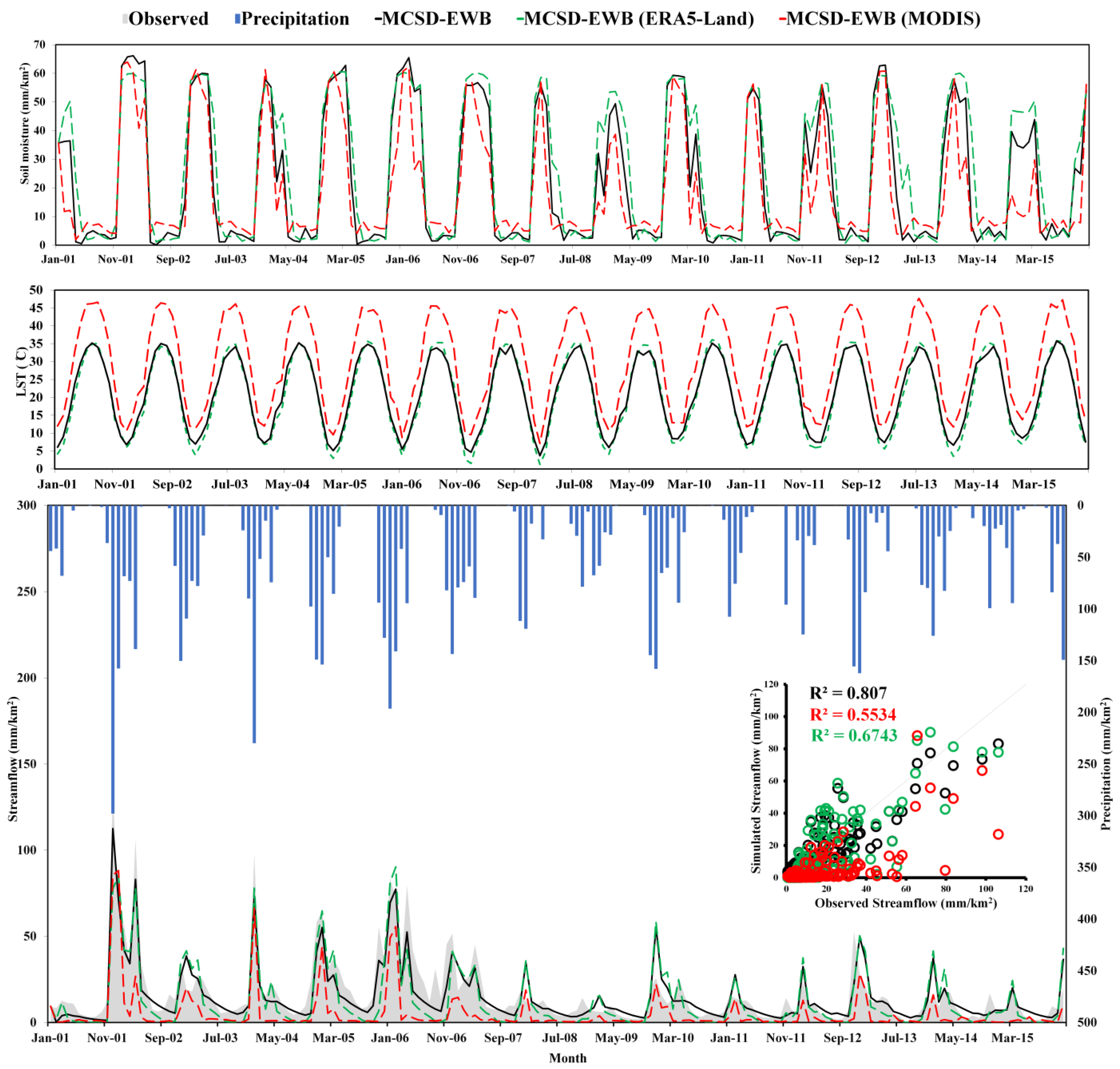
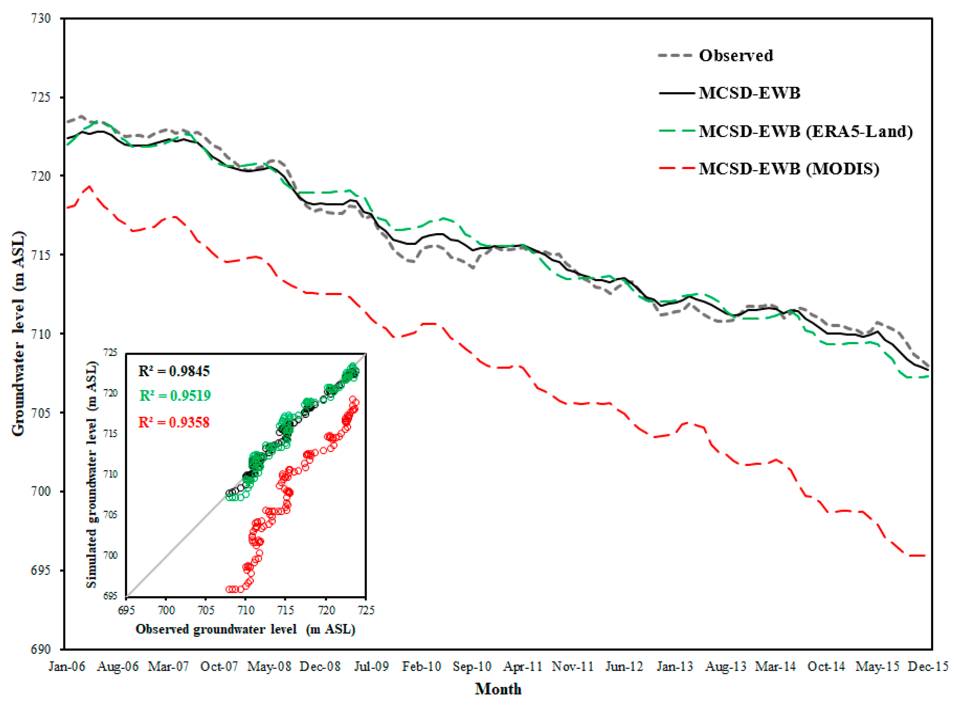
4.3. Behavioral Assessment Based on the Water Balance Model

The KGE, NSE, and RMSE values are presented for the MCSD-EWB, MCSD-EWB (ERA5-Land), and MCSD-EWB (MODIS) models for both streamflow and groundwater levels in Figure 9. Accordingly, the KGE values achieved for the MCSD-EWB, MCSD-EWB (ERA5-Land), and MCSD-EWB (MODIS) models are 0.98, 0.95, and 0.58, respectively. In addition, their NSE and RMSE values are [0.98, 0.98, and −2.15] and [1.02, 1.2, and 8.15], respectively. Therefore, the MCSD-EWB model has the best performance in simulating the groundwater time series, while the MCSD-EWB (ERA5-Land) and MCSD-EWB (MODIS) models have the second- and third-best performances, respectively. This conclusion is due to the higher ET values of the MCSD-EWB (MODIS) model than those of the MCSD-EWB and MCSD-EWB (ERA5_Land) models, which leads to a higher groundwater withdrawal and a more severe drop in the simulated groundwater level compared to the observed values. Regarding the results of the streamflow time series simulated by the MCSD-EWB, MCSD-EWB (ERA5-Land), and MCSD-EWB (MODIS) models, their KGE metrics are 0.75, 0.65, and −0.05, the NSE values are 0.7, 0.58, and −0.08, and the RMSE values are 10.2, 13.25, and 20.85, respectively. Therefore, the MCSD-EWB model, with the best statistical metrics in the simulation of streamflow, has the highest correlation with the observed values because it estimates ET more realistically than the other models, which leads to an accurate simulation of peak and baseflow values.

In conclusion, the MCSD-EWB model has the best performance in simulating both streamflow and groundwater levels, with the MCSD-EWB (ERA5-Land) and MCSD-EWB (MODIS) models ranking as the second- and third-best models, respectively, based on the statistical metrics.

4.4. Hydro-Climatic Conditions of the Watershed

The hydro-climatic conditions of the watershed include variations in streamflow, aquifer level, LST, soil moisture, and precipitation. To investigate these conditions, Figure 10 shows the time series of the monthly streamflow, LST, and soil moisture simulated by the MCSD-EWB, MCSD-EWB (ERA5-Land), and MCSD-EWB (MODIS) models, along with precipitation averaged over the watershed (during 2001–2015). Accordingly, the streamflow time series simulated using the MCSD-EWB and MCSD-EWB (ERA5-Land) models are in a suitable agreement with the values observed at the outlet of the watershed. The correlation coefficients of these models are 0.807 and 0.6743, respectively. The MCSD-EWB (MODIS) model has underestimated the streamflow time series in comparison with the observed values because of its large contribution of ET, which should be supplied by the water resources available in the watershed. This model, with an R² equal to 0.5534, has the third-best performance.

The temporal patterns of the simulated LST are similar for all three models. All of them show the largest temperature values in warm months and the lowest in cold months. The MCSD-EWB and MCSD-EWB (ERA5-Land) models have performed similarly in terms of LST magnitude, while the MCSD-EWB (MODIS) model has overestimated this by far among the models. The reason for this issue is because of the large proportion of soil within the sensor IFOV for a 5 km spatial resolution.

According to the results of soil moisture, all three models have reflected a similar temporal pattern. The highest soil moisture levels have occurred in cold and rainy months, and the lowest levels happened in warm and arid ones (inverse of the LST patterns). The differences between the three models are negligible in estimating the soil moisture magnitudes; however, the MCSD-EWB (MODIS) slightly has slightly underestimated and overestimated the magnitudes, respectively, for peaks and valleys compared with the other two models.

Figure 11 shows temporal variations in the monthly groundwater levels simulated by the MCSD-EWB, MCSD-EWB (ERA5-Land), and MCSD-EWB (MODIS) models against the observed values during 2006–2015. Regarding this figure, the MCSD-EWB and MCSD-EWB (ERA5-Land) models, with an R² equal to 0.9845 and 0.9519, respectively, have matched the observed values well. Meanwhile the MCSD-EWB (MODIS) model has underestimated the groundwater time series and has a poorer performance than the other two models, with an R² equal to 0.9358. The reason can be attributed to the high ET values simulated by the MCSD-EWB (MODIS) model, which requires groundwater withdrawal and surface and subsurface water resources to be supplied.

5. Conclusions

In the current research, a Monthly Continuous Semi-Distributed Energy Water Balance (MCSD-EWB) model has been developed to simulate the hydro-climatic conditions of a watershed. The proposed model is a monthly hydrological model based on a systematic semi-distributed combination of water and energy balances in which the surface energy and climatological water balance models were parameterized using a distributed approach, while the groundwater balance was parameterized using a lumped approach. According to the MCSD-EWB framework, the water–energy balance system has been solved as a function of EEBT, which denotes the land surface temperature, and a three-way simultaneous relationship has been formed between LST, surface soil moisture, and ET components. To implement the climatological water balance, groundwater balance, and ET models, the improved Jazim model, Mackay structure, and bulk transfer theory have been utilized, respectively. In addition to EEBT, the ERA5-Land and MODIS surface temperature retrievals have been utilized as inputs for the MCSD-EWB model to assess their performances.

According to the results, the performance of the MCSD-EWB and MCSD-EWB (ERA5-Land) models was found to be better than that of the MCSD-EWB (MODIS) model in simulating LST, streamflow, and aquifer levels versus the observed values. The temporal variations in streamflow and aquifer levels simulated by the MCSD-EWB and MCSD-EWB (ERA5-Land) models were in a suitable agreement with the observed time series, while the MCSD-EWB (MODIS) model underestimated the streamflow compared with the observations. This is primarily due to the estimation accuracy of ET, which is affected by the LST results. The LST achieved by the ERA5-Land dataset and MCSD model is more accurate than MODIS LST because the LST retrieval method is based on energy balance closure, which is a physical approach.

The temporal patterns of the simulated LST were similar in all the models, so that there was an increase in surface temperature values in warm, arid months and a decrease in cold, rainy months. In addition, the MCSD-EWB model was in better agreement with the MCSD-EWB (ERA5-Land) model in terms of the LST magnitude due to their similar approach in simulating LST. Similar to the land surface temperature, the temporal patterns of the simulated soil moisture were the same in all the models. The highest soil moisture values occurred in cold, rainy months and the lowest values in warm, arid months. Furthermore, the difference between the three models was insignificant in simulating the soil moisture magnitude.

Based on the results of the ET modeling, the maximum ET values obtained by the models occurred in the eastern parts of the watershed due to the forest vegetation cover. After that, these maximum values from the MCSD-EWB (ERA5-Land), MCSD-EWB, and MCSD-EWB (MODIS) models were observed at the grid point that included the dam (due to the high evaporation potential of the water body), the central region of the watershed (due to its extensive agricultural development), and southwestern areas surrounding the reservoir. The ET spatial patterns of the MCSD-EWB (ERA5-Land) model were more uniform than those of the other models and showed no distinction among the different parts of the watershed. In contrast, the MCSD-EWB and MCSD-EWB (MODIS) models depicted the changes in ET over the watershed well, and from this perspective, the results of these models were closer to each other than to the results of the MCSD-EWB (ERA5-Land) model. In addition, all models showed similar temporal behavior in simulating the ET; the largest ET values were related with MCSD-EWB (MODIS) and the lowest ones belonged to MCSD-EWB. It is worth noting that in terms of estimating the ET magnitude, the MCSD-EWB model performed closer to the MCSD-EWB (ERA5-Land) model than to the MCSD-EWB (MODIS) model.

Finally, the MCSD-EWB model had a suitable potential to simulate hydrological components by providing a flexible framework for fully interactive water and energy balances particularly in watersheds with a sparse ambient monitoring network, such as a synoptic station. Additionally, it indicated an acceptable performance in its spatiotemporal estimations of LST and ET. Thus, the proposed modeling structure can be an appropriate platform to develop distributed hydrological and water balance models, and its results may be used as good benchmarks to evaluate large-scale climatological data. Considering the flexible computation grid size, the proposed method could provide a suitable approach to the large-scale simulation of coupled energy and water balances.

References

1. McCabe, M.F.; Wood, E.F. Scale influences on the remote estimation of evapotranspiration using multiple satellite sensors. Remote Sens. Environ. 2006, 105, 271–285. [Google Scholar] [CrossRef]
2. Corbari, C.; Ravazzani, G.; Mancini, M. A distributed thermodynamic model for energy and mass balance computation: FEST–EWB. Hydrol. Process. 2011, 25, 1443–1452. [Google Scholar] [CrossRef]
3. Paciolla, N.; Corbari, C.; Hu, G.; Zheng, C.; Menenti, M.; Jia, L.; Mancini, M. Evapotranspiration estimates from an energy-water-balance model calibrated on satellite land surface temperature over the Heihe basin. J. Arid. Environ. 2021, 188, 104466. [Google Scholar] [CrossRef]
4. Kunnath-Poovakka, A.; Ryu, D.; Renzullo, L.J.; George, B. The efficacy of calibrating hydrologic model using remotely sensed evapotranspiration and soil moisture for streamflow prediction. J. Hydrol. 2016, 535, 509–524. [Google Scholar] [CrossRef]
5. Minacapilli, M.; Agnese, C.; Blanda, F.; Cammalleri, C.; Ciraolo, G.; D’Urso, G.; Iovino, M.; Pumo, D.; Provenzano, G.; Rallo, G. Estimation of actual evapotranspiration of Mediterranean perennial crops by means of remote-sensing based surface energy balance models. Hydrol. Earth Syst. Sci. 2009, 13, 1061–1074. [Google Scholar] [CrossRef] [Green Version]
6. Li, Z.L.; Tang, B.H.; Wu, H.; Ren, H.; Yan, G.; Wan, Z.; Sobrino, J.A. Satellite-derived land surface temperature: Current status and perspectives. Remote Sens. Environ. 2013, 131, 14–37. [Google Scholar] [CrossRef] [Green Version]
7. Lillesand, T.; Kiefer, R.W.; Chipman, J. Remote Sensing and Image Interpretation; John Wiley & Sons: Hoboken, NJ, USA, 2015. [Google Scholar]
8. Li, X.; Zhou, Y.; Asrar, G.R.; Zhu, Z. Creating a seamless 1 km resolution daily land surface temperature dataset for urban and surrounding areas in the conterminous United States. Remote Sens. Environ. 2018, 206, 84–97. [Google Scholar] [CrossRef]
9. Bastiaanssen, W.; Bandara, K.M.P.S. Evaporative depletion assessments for irrigated watersheds in Sri Lanka. Irrig. Sci. 2001, 21, 1–15. [Google Scholar] [CrossRef]
10. Hain, C.R.; Mecikalski, J.R.; Anderson, M.C. Retrieval of an available water-based soil moisture proxy from thermal infrared remote sensing. Part I: Methodology and validation. J. Hydrometeorol. 2009, 10, 665–683. [Google Scholar] [CrossRef]
11. Taheri, M.; Mohammadian, A.; Ganji, F.; Bigdeli, M.; Nasseri, M. Energy-based approaches in estimating actual evapotranspiration focusing on land surface temperature: A review of methods, concepts, and challenges. Energies 2022, 15, 1264. [Google Scholar] [CrossRef]
12. Corbari, C.; Mancini, M. Calibration and validation of a distributed energy–water balance model using satellite data of land surface temperature and ground discharge measurements. J. Hydrometeorol. 2014, 15, 376–392. [Google Scholar] [CrossRef]
13. Deardorff, J.W. Efficient prediction of ground surface temperature and moisture, with inclusion of a layer of vegetation. J. Geophys. Res. Ocean. 1978, 83, 1889–1903. [Google Scholar] [CrossRef] [Green Version]
14. Sellers, P.; Mintz, Y.; Sud, Y.E.A.; Dalcher, A. A simple biosphere model (SiB) for use within general circulation models. J. Atmos. Sci. 1986, 43, 505–531. [Google Scholar] [CrossRef]
15. Koster, R.D.; Suarez, M.J. Modeling the land surface boundary in climate models as a composite of independent vegetation stands. J. Geophys. Res. Atmos. 1992, 97, 2697–2715. [Google Scholar] [CrossRef]
16. Mahrt, L.; Ek, M. The influence of atmospheric stability on potential evaporation. J. Appl. Meteorol. Climatol. 1984, 23, 222–234. [Google Scholar] [CrossRef]
17. Jazim, A.A. A Monthly Six-parameter Water Balance Model and Its Application at Arid and Semiarid Low Yielding Catchments. J. King Saud Univ.-Eng. Sci. 2006, 19, 65–81. [Google Scholar] [CrossRef]
18. Mackay, J.D.; Jackson, C.R.; Wang, L. A lumped conceptual model to simulate groundwater level time-series. Environ. Model. Softw. 2014, 61, 229–245. [Google Scholar] [CrossRef] [Green Version]
19. Deardorff, J.W. Dependence of air-sea transfer coefficients on bulk stability. J. Geophys. Res. 1968, 73, 2549–2557. [Google Scholar] [CrossRef]
20. Peel, M.C.; Finlayson, B.L.; McMahon, T.A. Updated world map of the Köppen-Geiger climate classification. Hydrol. Earth Syst. Sci. 2007, 11, 1633–1644. [Google Scholar] [CrossRef] [Green Version]
21. Nasseri, M.; Zahraie, B.; Tootchi, A. Spatial scale resolution of prognostic hydrological models: Simulation performance and application in climate change impact assessment. Water Resour. Manag. 2019, 33, 189–205. [Google Scholar] [CrossRef]
22. Task, G.S.D. Global Soil Data Products CD-ROM Contents (IGBP-DIS); ORNL DAAC: Oak Ridge, TN, USA, 2014. [Google Scholar]
23. Lancaster, P.; Salkauskas, K. Surfaces generated by moving least squares methods. Math. Comput. 1981, 37, 141–158. [Google Scholar] [CrossRef]
24. Taheri, M.; Dolatabadi, N.; Nasseri, M.; Zahraie, B.; Amini, Y.; Schoups, G. Localized linear regression methods for estimating monthly precipitation grids using elevation, rain gauge, and TRMM data. Theor. Appl. Climatol. 2020, 142, 623–641. [Google Scholar] [CrossRef]
25. Amini, Y.; Nasseri, M. Improving spatial estimation of hydrologic attributes via optimized moving search strategies. Arab. J. Geosci. 2021, 14, 723. [Google Scholar] [CrossRef]
26. Balsamo, G.; Beljaars, A.; Scipal, K.; Viterbo, P.; van den Hurk, B.; Hirschi, M.; Betts, A.K. A revised hydrology for the ECMWF model: Verification from field site to terrestrial water storage and impact in the Integrated Forecast System. J. Hydrometeorol. 2009, 10, 623–643. [Google Scholar] [CrossRef] [Green Version]
27. Lhomme, J.P.; Chehbouni, A. Comments on dual-source vegetation–atmosphere transfer models. Agric. For. Meteorol. 1999, 94, 269–273. [Google Scholar] [CrossRef]
28. Crow, W.T.; Kustas, W.P.; Prueger, J.H. Monitoring root-zone soil moisture through the assimilation of a thermal remote sensing-based soil moisture proxy into a water balance model. Remote Sens. Environ. 2008, 112, 1268–1281. [Google Scholar] [CrossRef]
29. Martin, M.; Dickinson, R.E.; Yang, Z.L. Use of a coupled land surface general circulation model to examine the impacts of doubled stomatal resistance on the water resources of the American Southwest. J. Clim. 1999, 12, 3359–3375. [Google Scholar] [CrossRef]
30. Alfieri, J.G.; Niyogi, D.; Blanken, P.D.; Chen, F.; LeMone, M.A.; Mitchell, K.E.; Ek, M.B.; Kumar, A. Estimation of the minimum canopy resistance for croplands and grasslands using data from the 2002 International H2O Project. Mon. Weather Rev. 2008, 136, 4452–4469. [Google Scholar] [CrossRef]
31. Dickinson, R.E. Modeling evapotranspiration for three-dimensional global climate models. Clim. Process. Clim. Sensit. 1984, 29, 58–72. [Google Scholar]
32. Field, C.B.; Randerson, J.T.; Malmström, C.M. Global net primary production: Combining ecology and remote sensing. Remote Sens. Environ. 1995, 51, 74–88. [Google Scholar] [CrossRef] [Green Version]
33. Jahani, B.; Dinpashoh, Y.; Nafchi, A.R. Evaluation and development of empirical models for estimating daily solar radiation. Renew. Sustain. Energy Rev. 2017, 73, 878–891. [Google Scholar] [CrossRef]
34. Su, Z. The Surface Energy Balance System (SEBS) for estimation of turbulent heat fluxes. Hydrol. Earth Syst. Sci. 2002, 6, 85–100. [Google Scholar] [CrossRef]
35. Monteith, J.L. Gas exchange in plant communities. Environ. Control Plant Growth 1963, 95, 95–112. [Google Scholar]
36. Monin, A.S.; Obukhov, A.M. Basic laws of turbulent mixing in the surface layer of the atmosphere. Contrib. Geophys. Inst. Acad. Sci. USSR 1954, 151, e187. [Google Scholar]
37. Kutikoff, S.; Lin, X.; Evett, S.; Gowda, P.; Moorhead, J.; Marek, G.; Colaizzi, P.; Aiken, R.; Brauer, D. Heat storage and its effect on the surface energy balance closure under advective conditions. Agric. For. Meteorol. 2019, 265, 56–69. [Google Scholar] [CrossRef]
38. Heidkamp, M.; Chlond, A.; Ament, F. Closing the energy balance using a canopy heat capacity and storage concept–a physically based approach for the land component JSBACHv3. 11. Geosci. Model Dev. 2018, 11, 3465–3479. [Google Scholar] [CrossRef] [Green Version]
39. Liang, J.; Zhang, L.; Cao, X.; Wen, J.; Wang, J.; Wang, G. Energy balance in the semiarid area of the Loess Plateau, China. J. Geophys. Res. Atmos. 2017, 122, 2155–2168. [Google Scholar] [CrossRef]
40. Meyers, T.P.; Hollinger, S.E. An assessment of storage terms in the surface energy balance of maize and soybean. Agric. For. Meteorol. 2004, 125, 105–115. [Google Scholar]
41. Oncley, S.P.; Foken, T.; Vogt, R.; Kohsiek, W.; DeBruin, H.A.; Bernhofer, C.; Christen, A.; Van Gorsel, E.; Grantz, D.; Feigenwinter, C.; et al. The energy balance experiment EBEX-2000. Part I: Overview and energy balance. Bound.-Layer Meteorol. 2007, 123, 1–28. [Google Scholar] [CrossRef]
42. Nobel, P.S. Introduction to Biophysical Plant Physiology; Freeman: New York, NY, USA, 1974. [Google Scholar]
43. Guo, S.; Chen, H.; Zhang, H.; Xiong, L.; Liu, P.; Pang, B.; Wang, G.; Wang, Y. A semi-distributed monthly water balance model and its application in a climate change impact study in the middle and lower Yellow River basin. Water Int. 2005, 30, 250–260. [Google Scholar] [CrossRef]
44. Rabuffetti, D.; Ravazzani, G.; Corbari, C.; Mancini, M. Verification of operational Quantitative Discharge Forecast (QDF) for a regional warning system? the AMPHORE case studies in the upper Po River. Nat. Hazards Earth Syst. Sci. 2008, 8, 161–173. [Google Scholar] [CrossRef] [Green Version]
45. Duan, Q.; Sorooshian, S.; Gupta, V. Effective and efficient global optimization for conceptual rainfall-runoff models. Water Resour. Res. 1992, 28, 1015–1031. [Google Scholar] [CrossRef]
46. Mildrexler, D.J.; Zhao, M.; Running, S.W. A global comparison between station air temperatures and MODIS land surface temperatures reveals the cooling role of forests. J. Geophys. Res. Biogeosci. 2011, 116, G03025. [Google Scholar] [CrossRef]
47. Weng, Q.; Lu, D.; Schubring, J. Estimation of land surface temperature–vegetation abundance relationship for urban heat island studies. Remote Sens. Environ. 2004, 89, 467–483. [Google Scholar] [CrossRef]
48. Onwuka, B.; Mang, B. Effects of soil temperature on some soil properties and plant growth. Adv. Plants Agric. Res. 2018, 8, 34–37. [Google Scholar] [CrossRef]
Figure 1. The study region with its hydro-climatic stations, alluvial aquifer, and DEM. In more detail, plot A is satellite imagery of the watershed provided by Google Earth, demonstrating different land coverage. Plot B represents the topographical variations in the watershed along with the location of dams, hydrometric stations, aquifers, and rivers. Plot C illustrates a second-level watershed containing the study domain with climatologic stations.
Atmosphere 13 01916 g001
Figure 2. Schematic structure of MCSD-EWB model and exchanges of its energy and mass fluxes. The watershed has been divided into three parts, labeled 1, 2, and 3. The first part (labeled 1) includes karstic areas, and the climatological water balance and karst models have been implemented in spatially distributed and lumped ways, respectively. In the second part (labeled 2), the groundwater aquifer is located under the surface and unsaturated soil layers. Using the same method as that in the first part, climatological modeling has been conducted via a spatially distributed approach, and the groundwater model is a type of lumped model. The modeling process in the third area (labeled 3), which lacks karstic and alluvial aquifers, has been carried out via a distributed method. rb and rd are the boundary and turbulent diffusion resistances, respectively. Other parameters are defined in the next sections. In addition, hollow arrows show the input/output energy flows, and dashed and filled arrows show the direction of moisture in the conceptual model.
Atmosphere 13 01916 g002
Figure 3. Spatiotemporal patterns of long-term monthly average values of LST (°C) based on MCSD-EWB, MCSD-EWB (ERA5-Land), and MCSD-EWB (MODIS) models.
Atmosphere 13 01916 g003
Figure 4. Spatial patterns of the MAE metric (°C) between monthly EEBT and LST simulated by: (A) MCSD-EWB (MODIS) (B) MCSD-EWB (ERA5-Land) models.
Atmosphere 13 01916 g004
Figure 5. Boxplots of the RMSE metric (°C) between monthly EEBT and LST simulated by the MCSD-EWB (ERA5-Land) and MCSD-EWB (MODIS) models.
Atmosphere 13 01916 g005
Figure 6. Spatiotemporal changes in long-term monthly average of ET (mm) based on MCSD-EWB, MCSD-EWB (ERA5-Land), and MCSD-EWB (MODIS) models.
Atmosphere 13 01916 g006
Figure 7. Spatial distributions of MAE (mm) for the simulated monthly ET between the MCSD-EWB model and: (A) MCSD-EWB (MODIS) and (B) MCSD-EWB (ERA5-Land) models.
Atmosphere 13 01916 g007
Figure 8. Boxplots of RMSE (mm) for monthly ET between MCSD-EWB and other models (i.e., MCSD-EWB (MODIS), and MCSD-EWB (ERA5-Land)).
Atmosphere 13 01916 g008
Figure 9. NSE, KGE, and RMSE metrics of streamflow and groundwater levels simulated by the MCSD-EWB, MCSD-EWB (ERA5-Land), and MCSD-EWB (MODIS) models.
Atmosphere 13 01916 g009
Figure 10. Time series for monthly LST (°C), soil moisture (mm/km2), and streamflow (mm/km2) simulated by the MCSD-EWB, MCSD-EWB (ERA5-Land), and MCSD-EWB (MODIS) models, along with monthly precipitation and observed streamflow averaged over the watershed from 2001 to 2015.
Atmosphere 13 01916 g010
Figure 11. Time series of monthly groundwater level values simulated by the MCSD-EWB, MCSD-EWB (ERA5-Land), and MCSD-EWB (MODIS) models versus observational values during 2006–2015.
Atmosphere 13 01916 g011