Direct Detection of Severe Biomass Burning Aerosols from Satellite Data

Abstract

The boundary between high-concentration aerosols (haze) and clouds is ambiguous and the mixing of aerosols and clouds is complex in terms of composition and structure. In particular, the contribution of biomass burning aerosols (BBAs) to global warming is a source of uncertainty in the global radiation budget. In a previous study, we proposed a method to detect absorption aerosols such as BBAs and dust using a simple indicator based on the ratio of violet to near-ultraviolet wavelengths from the Global Change Observation Mission-Climate/Second-Generation Global Imager (GCOM-C/SGLI) satellite data. This study adds newly obtained SGLI data and proposes a method for the direct detection of severe biomass burning aerosols (SBBAs). Moreover, polarization data derived from polarization remote sensing was incorporated to improve the detection accuracy. This is possible because the SGLI is a multi-wavelength sensor consisting of 19 channels from 380 nm in the near-ultraviolet to thermal infrared, including red (674 nm) and near-infrared (869 nm) polarization channels. This method demonstrated fast SBBA detection directly from satellite data by using two types of wavelength ratio indices that take advantage of the characteristics of the SGLI data. The SBBA detection algorithm derived from the SGLI observation data was validated by using the polarized reflectance calculated by radiative transfer simulations and a regional numerical model—scalable computing for advanced library and environment (SCALE). Our algorithm can be applied to the detection of dust storms and high-concentration air pollution particles, and identifying the type of high-concentration aerosol facilitates the subsequent detailed characterization of the aerosol. This work demonstrates the usefulness of polarization remote sensing beyond the SGLI data.

1. Introduction

It is well-known that severe wildfires are not limited to equatorial regions but are increasing globally [1,2,3,4,5,6,7]. Wildfires not only cause extensive damage in the area where they occur but also in areas far from the fire [8,9,10]. Biomass burning aerosols (BBAs) can travel great distances, causing air pollution and posing a health hazard to humans [11,12,13,14]. Excessive air pollution due to events such as severe wildfires and desert dust storms [15,16] is still not fully understood. In urban areas, anthropogenic activities have led to an increased concentration of small harmful aerosols known as suspended particulate matter (PM2.5) [17,18]. Nevertheless, such severe haze events are often left as “undecided” pixels in satellite products because aerosol retrievals from passive satellite sensors are usually restricted to cloud-free scenes. Here, over 20 years of aerosol observations by satellite are briefly reviewed. Historically, the Total Ozone Mapping Spectrometer (TOMS) played an important role in aerosol remote sensing. The TOMS demonstrated that ultraviolet data were available for the detection of absorbing aerosols such as carbonaceous aerosols or mineral dust [19]. The imaginary part of the refractive index of an absorbing aerosol takes a large value. The moderate resolution imaging spectroradiometer (MODIS) is the most popular satellite-based tool for aerosol observations [20]. The polarization and directionality of the Earth’s reflectance (POLDER) is an innovative sensor for aerosol remote sensing. The POLDER has demonstrated the usefulness of polarization information for the analysis of aerosols [21], clouds, and aerosol above cloud systems [22].

The “undecided” pixels show the mixing phase of clouds and aerosols. It has been demonstrated that aerosols have various direct and indirect effects on the climate and that aerosols have negative effects on surface temperatures and positive effects on cloud cover [23,24]. Further knowledge of cloud formation and microphysics is necessary to address these problems [25]. In any case, retrieving aerosols in cloudy scenes is difficult but unavoidable. Aerosol modification due to fog and clouds has been reported from ground observation data over the years [26]. The spectral radiance measurements from the Scanning Imaging Absorption Spectrometer for Atmospheric Cartography (SCIAMACHY) have been examined to derive the aerosol contribution in cloudy scenes [27]. Rosenfeld has done a lot of excellent work on the impacts of cloud–aerosol interactions on cloud microstructure and precipitation by using a combination of in situ aircraft measurements, satellite remote sensing, and model simulations [28]. However, the uncertainty regarding radiative forcing through aerosol–clouds is still problematic [29]. Indeed, the boundary region between aerosols and clouds is a fascinating subject and their similarities and differences can be examined both theoretically and observationally.

As the first step in the original task of elucidating these high-concentration aerosols, this work proposes a method for the direct detection of severe wildfire-derived BBAs (SBBAs) from satellite data. The Japan Aerospace Exploration Agency’s Global Change Observation Mission-Climate (JAXA/GCOM-C) was launched on 23 December 2017, with a second-generation global imager (SGLI) on board. The SGLI is a 19-channel multispectral sensor with wavelengths ranging from near-ultraviolet (UV) to thermal infrared (IR), including red and near-IR polarization channels. Our recent work demonstrates that these features of the SGLI are useful for characterizing BBAs. The near-UV data are available for the detection of absorbing aerosols such as BBAs or dust [30]. The radiation simulation has been simplified by using the vector type radiative transfer equation because polarization information mainly represents the upper atmospheric field [31]. Furthermore, we show that SBBAs can be detected directly from SGLI data using these two unique SGLI features.

The remainder of this paper is organized as follows. Section 2 describes the method used to perform this study. The results of the SGLI data processing over the period 2018–2021 are described. Section 3 presents the specific results of SBBA detection according to the methods used in Section 2. In Section 4, the results are carefully examined from the standpoint of simulations with a regional numerical model—scalable computing for advanced library and environment (SCALE), and radiative transfer calculations [32,33,34]. Finally, a summary of the results and our future research plans are presented.

2. Method

2.1. Detection of SBBAs with SGLI Near-UV Data

The characteristics of aerosols can be represented by size and composition. Atmospheric aerosols are classified into six categories based on accumulated NASA/AERONET data: (1) biomass burning, (2) rural, (3) continental pollution, (4) dirty pollution, (5) desert dust, and (6) polluted marine [35]. We restricted our study to continental particles of natural origin, that is, BBAs and dust. Thus, identifying the aerosol type and cloud discrimination were performed using ADEOS-2/GLI data [30]. The ADEOS-2/GLI (Advanced Earth Observing Satellite-2/Global Imager) is the predecessor of the SGLI. BBAs and dust have the property of absorption at ultraviolet wavelengths. Using this property, TOMS extracted absorbing aerosols [19].

The term absorbing aerosol means large values for the imaginary part of the refractive index. Our absorbing aerosol index (AAI) followed the TOMS-AI (Aerosol Index) [19], but in a much simpler form, that is, the ratio of observed data alone [30]:

AAI = R(412)/R(380),

(1)

where R represents the reflectance observed by the SGLI at the near-UV (380 nm) and violet (412 nm) wavelengths. BBAs and dust aerosols are considered as they are typical examples of absorbing aerosols. The primary sources of BBAs and dust are wildfires and deserts, respectively. We chose the area over a large-scale wildfire outbreak as it was regarded as a proper candidate for the BBAs feasibility study. Figure 1 shows that between 2018 and 2021, the areas most affected by wildfires were North America, Amazon, South Africa, Siberia, and Southeast Asia, and the Sahara Desert emitted the most dust. We chose the GCOM-C/SGLI/level-2 data in the EQA format (sinusoidal equal area), with a resolution of 1/24 degrees (4.6 km). The number of total pixels for the BBAs was approximately 3,000,000. Note that the cloud pixels were excluded by using the GCOM-C/SGLI L2 cloud flag classification. As wildfires are a sudden natural phenomenon and are strictly limited to the area of intense wildfire, the data available for BBAs were less than those for dust. However, because we strictly selected severe wildfires, the contamination of other types of aerosols was reduced, and we considered this number of pixels to be sufficient for the statistical analysis of BBAs. On the other hand, the number of total pixels for dust was approximately 2,000,000.

Figure 2a,b show the results for BBAs while 2c and 2d are the results for dust. Figure 2a,c show the change in AAI values versus the aerosol optical thickness at 500 nm (AOT (500)) provided by JAXA/SGLI/L2/ver-2 for BBAs and dust. The AOT is the thickness of the atmosphere from an optical point of view. Note that the values of AOT > 5.0 are unavailable from SGLI/L2/ver-2 products; hence, the areas of AOT > 5.0 are colored grey. That is, the AOT ranges from 0 to 5. Figure 2b,d present the histograms of AAI pixel numbers. Figure 2a,c show that the most pixels are concentrated in AOT < 2. Furthermore, the surface reflection is no less than the scattering by atmospheric particles in AOT < 0.3 when the atmosphere is optically clear. Therefore, the histograms of the AAI pixel numbers are shown in Figure 2b,d. Additionally, histograms of the AAI divided into three parts (AOT ≤ 0.3, 0.3 < AOT ≤ 2, 2 < AOT ≤ 5) are presented in Figure 2(b1–b3) for BBAs and in Figure 2(d1–d3) for dust, where N, m, and σ denote the total number of data items (forest fires or dust pixels), mean value, and standard deviation, respectively. Figure 2(b1–b3,d1–d3) also show that many pixels have an AOT < 2.

From Figure 2, the following can be inferred:

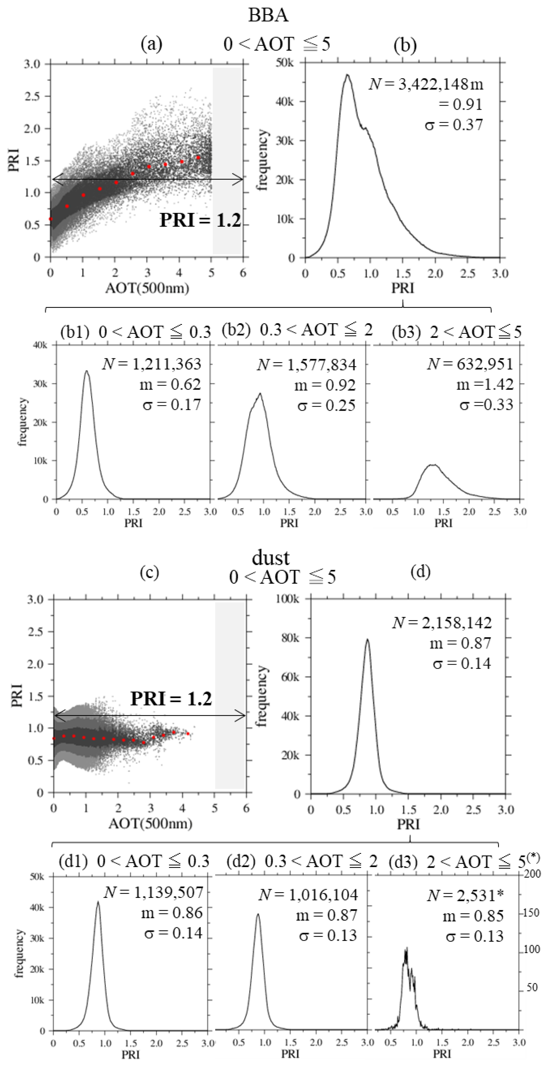
• For AOT ≤ 0.3, the effect of ground surface reflection can be seen (as the aerosols are optically thin and the ground can clearly be seen). In particular, for BBAs, the histograms show two peaks, indicating a difference in the AAI between reflected and scattered light. There is no apparent bimodal shape for dust, probably because dust aerosols are derived initially from desert soils and have the same wavelength characteristics.
• Most of the aerosols exist in AOT ≤ 2. As a result, AAI values are concentrated in this region, and the mean value for the entire AOT region is within 0.3 < AOT ≤ 2. This tendency is particularly strong in the case of dust, with almost all data falling within AOT ≤ 2. Therefore, the units on the vertical axis in Figure 2(d3) were changed. Naturally, it is necessary to take into account that the number of dust data items is only two-thirds that of the BBAs, that the data is limited to the Sahara Desert, and that it is challenging to retrieve the AOT from the satellite over the desert.
• The AAI values increase with AOT for BBAs and may exceed 1.1, around the limit value of AOT, which is 5. Then, BBAs with AOT (500) > 5, which are not derived in the official product, are referred to as SBBAs in this work.
• In the case of dust, the increasing trend in the AAI values with AOT stops around AOT = 2, converges, and never exceeds 1.1. Therefore, AAI = 1.1 can be regarded as a threshold that differentiates between SBBAs and dense dust. This is the intention of the arrows at both ends drawn in Figure 2a,c.

Our previous work revealed that the condition of AAΙ ≥ 0.83 indicates the presence of BBAs [31]. These results coincide with those presented in Figure 2a. Furthermore, the current study shows that the AAI would have a value of 1.1 or higher in the case of SBBAs. Notably, the AAI values of BBAs increased with optical thickness, while those of dust show similar behavior with optical thickness but they converge around AOT = 2, suggesting that AAI ≥ 1.1 helps to detect extremely severe biomass burning aerosols.

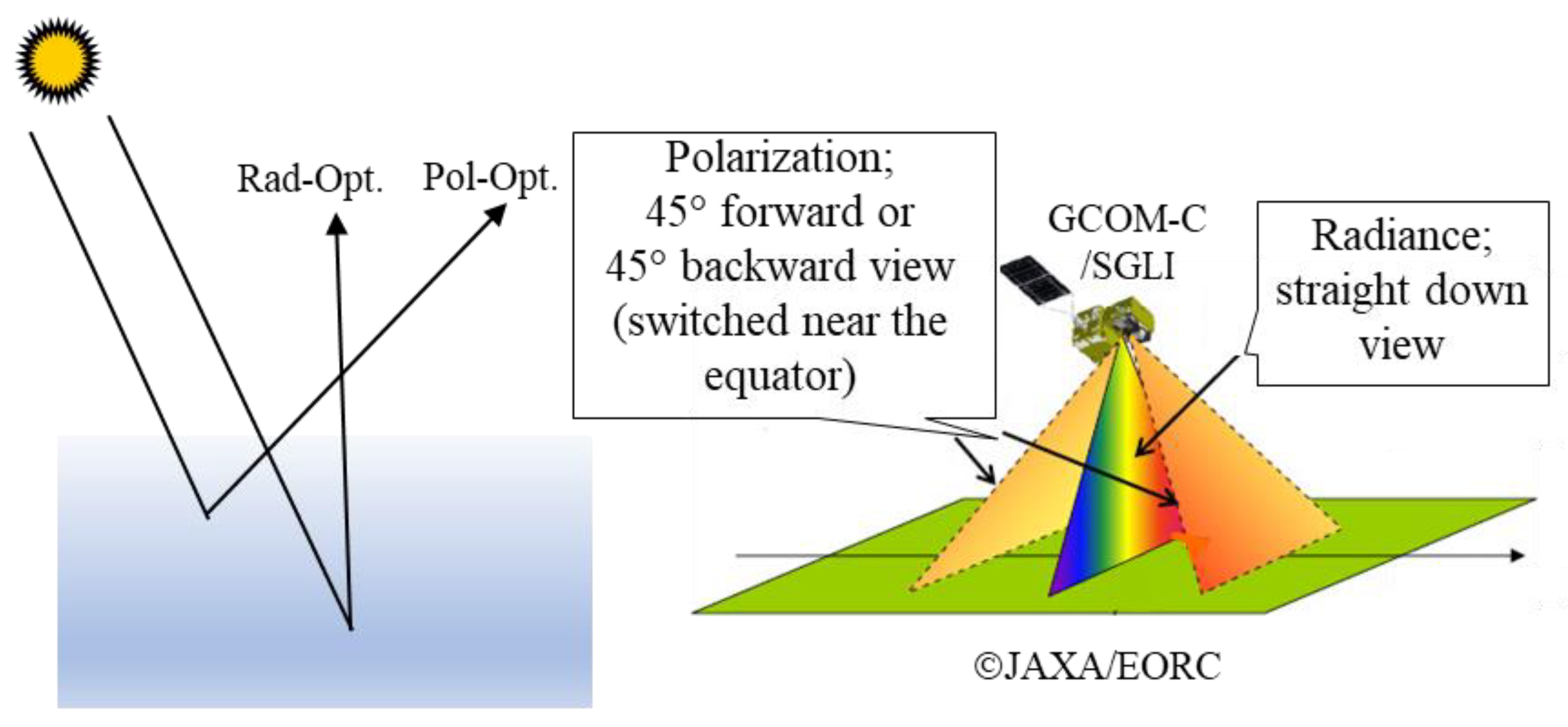
2.2. Detection of SBBAs with Polarized Radiance

GCOM-C/SGLI is a multi-channel sensor that includes near-ultraviolet wavelengths that can observe various geophysical parameters including not only aerosol properties, but also cloud, land cover, land biomass, ocean biomass, and coastal changes. Thus, it can detect SBBAs using the indicator AAI defined in Equation (1); however, it has already been in operation for five years. Therefore, it is necessary to develop and operate a successor to the SGLI, and an alternative to the indicator AAI should also be considered. The SGLI is a follow-on sensor in the POLDER series of ADEOS-1, -2, and PARASOL and it has unique capabilities for measuring polarization [19,21]. It was designed to acquire scattered light Stokes vector parameters (I, Q, and U) at moderate scattering angles (approximately 90–120°) with a 45° back and forth tilt observation at two wavelengths, red and near-IR. Polarization information provides new opportunities for future Earth observation satellite data applications and a return to the polarization remote sensing era. First, it is expected to be applied to EU-METSAT/EPS-SG/3MI, which is scheduled to be launched in 2024 [22]. In addition, it would be useful to validate the AAI index if another detection method for SBBAs could be devised.

Figure 3 is the same as Figure 2 but for the ratio of polarized radiance (PRI), which is defined as

PRI = PR(869)/PR(674),

(2)

where PR represents the polarized radiance of reflectance observed by the SGLI defined in the case of Stokes parameters (I, Q, U, V) at the wavelength (λ) as

$$\mathrm{PR}\left(\mathsf{\lambda }\right)=\sqrt{\mathrm{Q}{(\mathsf{\lambda })}^2+\mathrm{U}{(\mathsf{\lambda })}^2},$$

(3)

As shown in Figure 3, the typical values of PRI for the dust aerosols did not change much with AOT. The PRI in AOT ≤ 2 has large variations, occasionally reaching as high as 1.5, while that in AOT > 2 tends to converge to a smaller value. On the other hand, PRI values for BBAs increase with AOT, exceeding 1.2 for AOT > 2, and they show a tendency for PRI ≥ 1.2 cases to increase with AOT. This indicates that if AOT > 5, the PRI value of SBBAs is more than 1.2.

Figure 4 presents the scatterplots for AAI and PRI. For BBAs, AAI, and PRI have a linear proportional relationship (see Figure 4a and the correlation coefficient γ). However, in the case of dust (Figure 4b), the linear relationship between the two indices is not clear, AAI and PRI. Figure 4c is a superimposed image of Figure 4a,b. Here, red represents BBAs, blue represents dust, and green represents the area where the two overlap. In other words, the AAI and PRI in the green region are not useful for separating BBA and dust, and denote “not identifiable.” It was observed in Figure 2 that AAI increases with AOT. The SBBAs are referred to as BBAs with AOT (500) > 5. Therefore, the lower red part in Figure 4c represents the BBAs and the upper SBBAs.

3. Specific Results of SBBA Detection

Figure 5 presents the biomass burning events captured by GCOM-C/SGLI on 12 September 2022, in western North America. Figure 5a is a color composite image in which the three primary colors (R, G, B) correspond to the usual (674, 530, 443 nm) wavelength bands, and a large amount of smoke from the wildfire is clearly visible. The red and orange dots represent the hotspots on 11 and 12 September 2020, respectively, obtained from Terra/MODIS [36]. Note that the transit time of Terra is 19:35 (UTC) and that of GCOM-C is around 19:11. Although the transit times of both satellites are nearly identical, the smoke in the SGLI image on September 12 originated from fire prior to the SGLI observation. Figure 5b presents the AOT (500) derived from JAXA/SGLI/L2/ver-2, where the definite clouds are denoted by gray, and the white pixels represent uncertain pixels, namely, those left as “uncertain” pixels in JAXA/SGLI/L2/ver-2 products. These uncertain white-colored pixels represent pixels with an AOT > 5.0 and pixels with an undetermined AOT due to various causes, such as the complex structure of the ground surface and cloud shadow. The latter can be inferred from the quality assurance (QA) flag of the SGLI/L2 aerosol product. Figure 5c shows the results obtained by subtracting these pixels from the total number of uncertain pixels to obtain the pixels corresponding to AOT > 5.0 (hereafter named SBBAs candidate pixels for convenience). In other words, these pixels may indicate the presence of optically dense aerosols, the SBBAs from wildfires that are the target of this study. The light pink color in Figure 5c represents those candidate pixels that exist for SBBAs. The red squares in Figure 5b denote the NASA/AERONET stations for reference [37]. Several AERONET sites exist in our target area. The ground observation data from NASA/AERONET is valuable and indispensable for validating the characteristics of the atmospheric particles from satellite observations [34].

Figure 6a presents the distribution of AAI obtained from the SGLI over the same area as that shown in Figure 5b. Figure 6b, a clipped version of Figure 6a, shows the candidate areas for SBBAs (denoted by light pink in Figure 5c), and the definite clouds defined with JAXA/SGLI/L2/ver-2 are represented by gray. Note that the color scale of Figure 6b is enlarged to [1.0, 1.2] from [0.8, 1.3] in Figure 6a to make the SBBA candidate area more detailed for clarity. The pixels with lower values than the threshold of the AAI for the indication of SBBAs, i.e., AAI = 1.1, are denoted by green. There is a substantial number of green pixels on the periphery of the SBBA candidate area. This is also confirmed in Figure 2a, where AAI = 1.1 is close to the upper limit in the SGLI/BBA sampling data. In other words, a pixel that meets the requirements of AAI ≥ 1.1 meets the rigorous requirements for SBBA certification. Figure 6c,d are the same as Figure 6a,b, respectively, but for PRI, it can be seen that there are no green pixels at all. Almost all of the candidate pixels for SBBAs satisfy the condition of PRI ≥ 1.2. These results are consistent with those presented in Figure 3a. This shows that BBAs may satisfy the condition of PRI ≥ 1.2 even if the AOT is not so high. Figure 6 shows that the pixels satisfying the conditions of AAI ≥ 1.1 and PRI ≥ 1.2 meet the necessary and sufficient conditions for SBBA detection. This is also indicated in Figure 4a, which presents a clear linear relationship between AAI and PRI. The condition of AAI ≥ 1.1 is more demanding for the detection of SBBAs, at least in this scenario. The AAI ≥ 1.1 pixels in Figure 6b can be identified as SBBAs. For the detection of SBBAs, only AAI is required, meaning that the indicator PRI is useless or an auxiliary condition; however, there could be more. This point, including the usefulness of polarization information, is addressed in the next section. There is no strict delineation of SBBAs. In this study, we are merely using SBBAs to indicate highly optically thick BBA particles. From this perspective, the green area in Figure 6b is of great interest as a transition zone or a mixing zone from BBA to SBBAs. It would be preferable to assume that the candidate site for SBBAs satisfies AAI ≥ 1.1 or PRI ≥ 1.2.

Of note, there is no discontinuity between the cloud and SBBA regions, as shown in Figure 6a,c. For reference, the distribution of the cloud optical thickness (COT (500nm)) obtained from the SGLI/L2/ver.2 product is shown in Figure 6e. The COT values are almost equivalent to those of the AOT in Figure 5b. Figure 6f is a superimposed view of both. Figure 6a,c,f show that there is no clear boundary between aerosols and clouds and that the quantity of each is continuously distributed. This suggests that very thick BBAs or SBBAs cover the land area in the upper center half of Figure 6. In particular, the PRI distribution in Figure 6c strongly indicates that this is the situation. Polarization information is considered in the next section. In the discussion below, the small black square represents the NASA/AERONET site PNNL and the black circle indicates a point in the cloud.

4. Discussion: Role of Polarization

Here, we consider polarization more carefully. Figure 7 compares the SGLI measurements with the wind speed and direction simulated by the numerical regional model, SCALE over the same area as Figure 5a on 12 September 2020. Figure 7a–d show the images from the SGLI measurement over the same scene as Figure 5a at wavelengths of 674 and 869 nm. The PR is shown in Figure 7a,b, and R is shown in Figure 7c,d at wavelengths of 674 and 869 nm. The radiance images correspond well to the color composite image in Figure 5a. Typically, AOT decreases with wavelength, and the amount of light scattered decreases; hence, the R at the top of the atmosphere decreases, but the distribution pattern of the radiance is maintained. On the contrary, the polarized radiance image in Figure 7a,b show a different pattern. Considering the wavelength dependence of AOT, Figure 7a,b show that the polarized radiance reflects the aerosol properties of the optically thin atmosphere or those in the upper atmosphere. For more clarity, the wind behavior at 10 m above the ground and at 500 hPa from 15:00 to 19:00 (UTC), which is approximately 10 min before the SGLI passage, has been simulated by a regional numerical model—SCALE with a 30 × 30 km resolution [34]. Figure 7e shows the time-averaged value of the wind at 500 hPa (corresponding to an altitude of about 5500 m) from 15:00 to 19:00 (UTC). Figure 7f shows the same wind behavior as that in Figure 7e at 10 m above the ground. It can be seen how the wind from the southwest to the northeast carries the wildfire smoke, as indicated by the many hot spots, which are denoted by orange dots in the lower left to the upper right. The small black square in Figure 7 denotes the NASA/AERONET site PNNL. The PR reflects the upper atmosphere motion well (Figure 7e), and the R reflects the accumulated atmospheric dynamics (Figure 7f). PR is sensitive to phenomena on a short space scale, even in a very optically thick atmosphere. That is, polarization information is useful for understanding aerosols in the upper layer of the atmosphere at the time of observation.

Radiative transfer calculations in the polarized radiation field of the combined system of Earth’s atmosphere and Lambert’s bottom surface would help us understand the issues discussed above, namely, the roles of polarized radiation and radiance in satellite observation analysis. Figure 8a,b present the numerical results of PR and R, respectively, at a wavelength of 674 nm and 869 nm, denoted by the dashed curve and the dotted one, respectively, from radiative transfer simulations in the Stokes vector field (I, Q, U, V) against AOT (500 nm). For reference, AOT (674 nm) and AOT (869 nm) corresponding to AOT (500 nm) are shown at the bottom table outside the frame of Figure 8a. Of note, Figure 8 is just an example of the simulated results of radiative transfer for validating the SGLI data analysis presented in Figure 2 and Figure 3. However, the directional information in Figure 8 uses an AERONET/PNNL site on 12 September 2020 (see Figure 7 and Figure 9). The characteristics of BBAs, especially the complex refractive index, have been actively discussed in recent years in terms of observation, experiment, and theory; these are briefly reviewed in the next section, although the basic BBA model [38] is used in Figure 8. The solid curve in Figure 8a represents the PRI calculated by Equation (2) using numerical values of the simulated PR (674) and PR (869). Figure 8 shows:

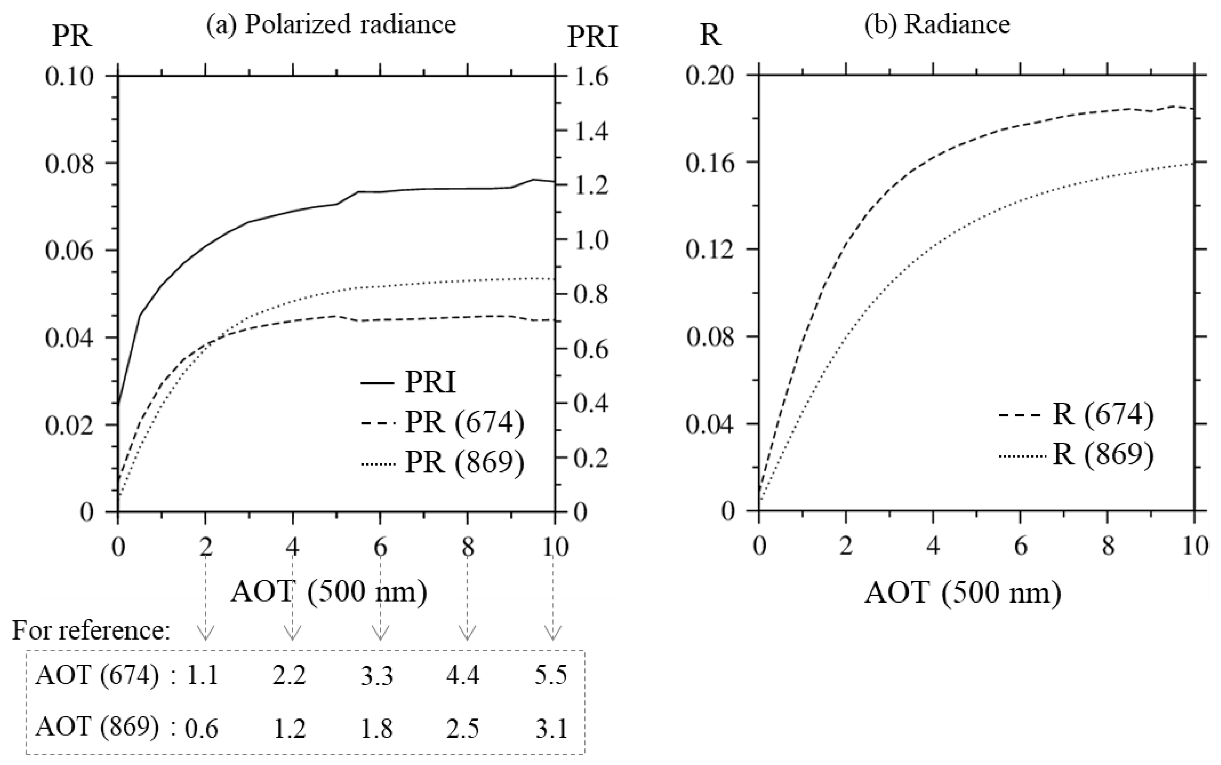
• The value of the PR (674) increases with AOT up to AOT (500) ≈ 2 (i.e., AOT (674) ≈ 1) while maintaining a higher value than PR (869) and then converging to a constant value;
• The value of the PR (869) increases with AOT up to AOT (500) ≈ 4 (i.e., AOT (869) ≈ 1) and continues to increase slowly thereafter. The PR (869) has higher values than PR (674) after AOT (500) ≈ 2;
• The resulting PRI, the ratio of the PR (869) to PR (674), exceeds 1 after AOT (500) ≈ 2 and has a value of 1.2 at AOT (500) = 10, the maximum value of AOT (500) in Figure 8;
• The R values at both wavelengths increase with AOT.

The specific values depend on the BBA model, but the trend in Figure 8 remains the same. This has been confirmed by other BBA models with different sizes and refractive indices. Thus, the PR begins to saturate when AOT (λ) exceeds one, suggesting that the PR reflects the optical properties of the upper atmosphere even in an optically thick atmosphere. Therefore, it makes sense that the upper atmospheric wind behavior in Figure 7e is similar to the PR distributions in Figure 7a,b, as already noted above. On the contrary, R increases with AOT, although the rate of increase depends on λ. Radiative transfer calculations equivalent to the AAI were not made here because of the strong dependence of the BBA model on the refractive index at short wavelengths. However, it is also convincing because the distribution of the satellite-observed R shown in Figure 7c,d is consistent with the behavior of the ground surface winds. Based on the above, it can be stated that PRI > 1.2 has been validated as an indicator for detecting SBBAs.

Figure 9 shows the measurements at the NASA/AERONET/PNN site on 12 September 2020, when the Ångströme Exponent (AE) takes around 1.63 as a reference. If the goal is to derive aerosol properties, the aerosol model needs to be more rigorously described and optimized for measurements at PNNL NASA/AERONET sites by varying the characteristic parameters. As this work aims to propose an index for detecting SBBA candidate pixels directly from satellite data, as a preliminary step for exact aerosol characterization, we adopted a basic BBA model [39] rather than one specific to the object of analysis. For example, the small black circles in Figure 6c,d,f point to a pixel in the water cloud. That pixel has a COT(500) ≈ 6.4. Similarly, the small black squares in Figure 6c–e denote AERONET/site PNNL, for which AOT values have not been determined in the official product from JAXA/SGLI/ver.2 due to an AOT (500) > 5. Ground measurements at the NASA/AERONET/PNNL site suggest a larger AOT (500) value than 5.0 (refer to Figure 9). However, there is no discontinuity between the black circles and black squares in the distribution plots in Figure 6c–f. The numerical results in Figure 8 also indicate a smooth transition from optically thick aerosols to thin clouds. This may suggest the need to treat the coexistence and mixing of clouds and aerosols as a whole rather than treating clouds and aerosols as separate phenomena. This is an urgent and necessary task but highly challenging. First, it is essential to describe the geometry of the mixed state of the two and elucidate their optical and chemical properties before radiative transfer computations.

5. Summary and Future Plans

In this study, we proposed two efficient indices: AAI, as found by Equation (1) and PRI, as found by Equation (2) to detect SBBAs caused by wildfires directly from satellite observations by utilizing GCOM-C/SGLI, which can simultaneously observe radiance and polarization, and we attempted to demonstrate their utilization from various standpoints. By first detecting the existence of SBBAs, the preparation of detailed BBAs models can be facilitated based on the satellite data before aerosol retrieval, where our algorithm has been described in detail in previous work [34]. Wildfires have usually been thought of as local, short-term phenomena [40,41]; however, in recent years, large-scale forest fires have become more frequent in many parts of the world. It is well-known that the long-distance transport of smoke particles significantly impacts air pollution and global warming [9]. Thus, the optical properties of aerosols derived from wildfires, as discussed here, have been recognized, and their chemical and microphysical properties are frequently referred to [42,43,44,45,46,47,48,49]. The next challenge is to achieve aerosol retrieval that considers the characteristics of this multifaceted BBA model. As updrafts accompany forest fires, the generated aerosol particles flow to higher altitudes. A number of reports indicate that up to about 30% of fire plumes over North America have reached the free troposphere [50]. Plumes that are sufficiently buoyant due to the affective air currents of the fire tend to be trapped near stratified stable layers. Aerosols injected at high altitudes significantly impact atmospheric chemistry and climate [51]. The polarization information is also useful for understanding the dynamics of aerosols in the upper layer. In the future, we would like to compare the results of our simulations with those of chemical transport models. Our challenge is to introduce a more realistic description of wildfires into the regional numerical model.

Our intention in focusing on optically thick aerosol events (SBBAs) was to take the opportunity to clarify the boundary between clouds and aerosols or the mixing region [26]. In addition, we wanted to demonstrate the usefulness of polarization information as a means of achieving this. Figure 10 illustrates how the multidirectional observation data of radiance can be obtained by using the different observation barrel angles of the SGLI radiation observation optics and polarization optics. Figure 10 shows how both the radiance optics and polarization optics of the SGLI can be used to obtain multidirectional observation data for radiance. As shown in the figure, the radiance optics takes a straight down view, and the polarization optics take an oblique observation of ±45° (the switch between 45° and −45° is made above the equator) [52]. We want to capture the geometric attributes of the atmosphere based on the multidirectional information of R in addition to information on the upper atmosphere, which is a characteristic of PR. The SGLI multidirectional database is currently being prepared for this purpose. Once the candidate area for SBBAs has been selected, we can continue to the characterization step of the BBAs around the SBBA area. An example of this task has already been described in our previous work [34]. However, at that time, the detection of SBBAs was only performed using AAI values based on SGLI data for the two-year period from 2018 to 2019. In this paper, we have added newly obtained SGLI data for 2020 and 2021, as well as the AAI and PRI index using polarization data to further improve the detection of SBBAs. We are currently refining the processing steps and RT methods in order to extend the derivation of aerosol properties over a wider range of regions and days. Above all, we aim to obtain geometric information by taking advantage of multi-directional data rather than limiting it to the cases described in this work. If we can obtain cross-sectional observation information, we expect to capture the growth process of aerosols to clouds and the layer structure of clouds and aerosols (aerosols above clouds and the aerosol layer below clouds). Then, the numerical model simulation can be of great help.

References

1. Stohl, A.; Berg, T.; Burkhart, J.F.; Fjaraa, A.M.; Forster, C.; Herber, A.; Hov, O.; Lunder, C.; McMillan, W.W.; Oltmans, S.; et al. Arctic smoke record air pollution levels in the European Arctic during a period of abnormal warmth, due to agricultural fires in Eastern Europe. Atmos. Chem. Phys. 2007, 7, 511–534. [Google Scholar] [CrossRef] [Green Version]
2. Markar, P.; Akingunola, A.; Chen, J.; Pabla, B.; Gong, W.; Stroud, C.; Sioris, C.; Anderson, K.; Cheung, P.; Zhang, J.; et al. Forest fire aerosol- weather feedback over western North America using a high-resolution, fully coupled, air quality model. Atmos. Chem. Phys. 2020, 21, 10557–10587. [Google Scholar] [CrossRef]
3. IPCC. Climate Change 2021: The Physical Science Basis; Contribution of working group I to the sixth assessment report of the Intergovernmental Panel on Climate Change; Cambridge University Press: Cambridge, UK, 2021. [Google Scholar]
4. Konovalov, I.; Golovushkin, N.; Beekmann, M.; Turquety, S. Using multi-platform satellite observations to study the atmospheric evolution of brown carbon in Siberian biomass burning plumes. Remote Sens. 2022, 14, 2625. [Google Scholar] [CrossRef]
5. Tan-Sooa, J.-S.; Pattanayak, S.K. Seeking natural capital projects: Forest fires, haze, and early-life exposure in Indonesia. Proc. Natl. Acad. Sci. USA 2019, 116, 5239–5245. [Google Scholar] [CrossRef] [PubMed] [Green Version]
6. Sastry, N. Forest fires, air pollution, and mortality in Southeast Asia. Demography 2002, 39, 1–23. [Google Scholar] [CrossRef] [PubMed]
7. Sahu, R.K.; Hari, M.; Tyagi, B. Forest fire induced air pollution over Eastern India during March 2021. Aerosol Air Qual. Res. 2022, 22, 220084. [Google Scholar] [CrossRef]
8. Poulos, G.; Pielke, R. A numerical analysis of Los Angeles basin pollution transport to the Grand Canyon under stably stratified Southwest flow conditions. Atmos. Environ. 1994, 28, 3329–3357. [Google Scholar] [CrossRef]
9. Sayer, A.; Hsu, N.; Eck, T.; Smirnov, A.; Holben, B. AERONET-based models of smoke-dominated aerosol near source regions and transported over ocean, and implications for satellite retrievals of aerosol optical depth. Atmos. Chem. Phys. 2014, 14, 11493–11523. [Google Scholar] [CrossRef] [Green Version]
10. Dickman, K. The hidden toll of wildfire. Sci. Am. 2020, 322, 38–45. [Google Scholar]
11. Liu, J.C.; Pereira, G.; Uhl, S.A.; Bravo, M.A.; Bell, M.L. A systematic review of the physical health impacts from non-occupational exposure to wildfire smoke. Environ. Res. 2015, 136, 120–132. [Google Scholar] [CrossRef] [PubMed] [Green Version]
12. Cascio, W.E. Wildland fire smoke and human health. Sci. Total Environ. 2018, 624, 586–595. [Google Scholar] [CrossRef]
13. Rappold, A.G.; Stone, S.L.; Cascio, W.E.; Neas, L.M.; Kilaru, V.J.; Carraway, M.S.; Vaughan-Batten, H. Peat bog wildfire smoke exposure in rural North Carolina is associated with cardiopulmonary emergency department visits assessed through syndromic surveillance. Environ. Health Perspect. 2011, 119, 1415. [Google Scholar] [CrossRef] [PubMed] [Green Version]
14. Reid, C.E.; Brauer, M.; Johnston, F.H.; Jerrett, M.; Balmes, J.R.; Elliott, C.T. Critical review of health impacts of wildfire smoke exposure. Environ. Health Perspect. 2016, 124, 1334–1343. [Google Scholar] [CrossRef] [Green Version]
15. Li, F.; Vogelmann, A.; Ramanathan, V. Saharan dust aerosol radiative forcing measured from space. J. Clim. 2004, 17, 2558–2571. [Google Scholar] [CrossRef]
16. Lee, K.; Kim, Y. Satellite remote sensing of Asian aerosols: A case study of clean, polluted and dust storm days. Atmos. Meas. Tech. 2010, 3, 1771–1784. [Google Scholar] [CrossRef] [Green Version]
17. Diemoz, H.; Barnaba, F.; Magri, T.; Pession, G.; Dionisi, D.; Pittavino, S.; Tombolato, I.K.F.; Campanelli, M. Sofia, L.D.C.; Hervo, M.; et al. Transport of Po Valley aerosol pollution to the northwestern Alps—Part 1: Phenomenology. Atmos. Chem. Phys. 2019, 19, 3065–3095. [Google Scholar] [CrossRef] [Green Version]
18. Hu, W.; Zhao, T.; Bai, Y.; Shen, L.; Sun, X.; Gu, Y. Contribution of regional PM2.5 transport to air pollution enhanced by sub-basin topography, A modeling case over Central China. Atmosphere 2020, 11, 1258. [Google Scholar] [CrossRef]
19. Torres, O.; Bhartia, P.K.; Herman, J.R.; Ahmad, Z. Derivation of aerosol properties from satellite measurements of backscattered ultraviolet radiation: Theoretical basis. J. Geophys. Res. 1998, 103, 17099–17110. [Google Scholar] [CrossRef]
20. King, M.; Menzel, P.; Kaufman, Y.; Tanré, D.; Gao, B.; Platnick, S.; Ackerman, S.; Remer, L.; Oincus, R.; Hubanks, P. Cloud and aerosol properties, precipitable water, and profiles of temperature and water vapor from MODIS. IEEE Trans. Geosci. Remote Sens. 2003, 41, 442–458. [Google Scholar] [CrossRef] [Green Version]
21. Deuze’, J.; Bre’on, F.; Devaux, C.; Goloub, P.; Herman, M.; Lafrance, B.; Maignan, F.; Marchand, A.; Nadal, F.; Perry, G.; et al. Remote sensing of aerosols over land surfaces from POLDER/ADEOS-1 polarized measurements. J. Geophys. Res. 2001, 106, 4913–4926. [Google Scholar] [CrossRef] [Green Version]
22. Waquet, F.; Cornet, C.; Deuz’e, J.; Dubovik, O.; Ducos, F.; Goloub, P.; Herman, M.; Lapyonok, T.; Labonnote, L.; Riedi, J.; et al. Retrieval of aerosol microphysical and optical properties above liquid clouds from POLDER/PARASOL polarization measurements. Atmos. Meas. Tech. 2013, 6, 991–1016. [Google Scholar] [CrossRef]
23. Liao, H.; Seinfeld, J. Effect of clouds on direct aerosol radiative forcing of climate. J. Geophys. Res. 1998, 103, 3781–3788. [Google Scholar] [CrossRef]
24. Quaas, J.; Boucher, O.; Bellouin, N.; Kinne, S. Satellite-based estimate of the direct and indirect aerosol climate forcing. J. Geophys. Res. 2008, 113, D05204. [Google Scholar] [CrossRef]
25. Ten Hoeve, J.E.; Remer, L.A.; Jacobson, M.Z. Microphysical and radiative effects of aerosols on warm clouds during the Amazon biomass burning season as observed by MODIS impacts of water vapor and land Cover. Atmos. Chem. Phys. 2011, 11, 3021–3036. [Google Scholar] [CrossRef] [Green Version]
26. Eck, T.; Holben, B.; Reid, J.; Giles, D.; Rivas, M.; Singh, R.; Tripathi, S.; Bruegge, C.; Platnick, S.; Arnold, G.; et al. Fog- and cloud-induced aerosol modification observed by the Aerosol Robotic Network (AERONET). J. Geophys. Res. 2012, 117, D07206. [Google Scholar] [CrossRef]
27. De Graaf, M.; Stammes, P.; Aben, E. Analysis of reflectance spectra of UV-absorbing aerosol scenes measured by SCIAMACHY. J. Geophys. Res. 2007, 112, D02206. [Google Scholar] [CrossRef] [Green Version]
28. Rosenfeld, D.; Sherwood, S.; Wood, R.; Donner, L. Climate effects of aerosol-cloud interactions. Science 2014, 343, 379–380. [Google Scholar] [CrossRef] [PubMed]
29. Rosenfeld, D.; Zhu, Y.; Wang, M.; Zheng, Y.; Goren, T.; Yu, S. Aerosol-driven droplet concentrations dominate coverage and water of oceanic low-level clouds. Science 2019, 363, 6427. [Google Scholar] [CrossRef] [Green Version]
30. Mukai, S.; Sano, I.; Nakata, M. Algorithms for the classification and characterization of aerosols: Utility verification of near-UV satellite observations. J. Appl. Rem. Sens. 2019, 13, 014527. [Google Scholar] [CrossRef] [Green Version]
31. Mukai, S.; Sano, I.; Nakata, M. Improved algorithms for remote sensing-based aerosol retrieval during extreme biomass burning. Atmosphere 2021, 12, 403. [Google Scholar] [CrossRef]
32. Nishizawa, S.; Yashiro, H.; Sato, Y.; Miyamoto, Y.; Tomita, H. Influence of grid aspect ratio on planetary boundary layer turbulence in large-eddy simulations. Geosci. Model Dev. 2015, 28, 3393–3419. [Google Scholar] [CrossRef]
33. Kajino, M.; Deushi, M.; Sekiyama, T.; Oshima, N.; Yumimoto, K.; Tanaka, T.Y.; Ching, J.; Hashimoto, A.; Yamamoto, T.; Ikgami, M.; et al. NHM-Chem, Japan Meteorological Agency’s Regional Meteorology—Chemistry Model: Model Evaluations Toward the Consistent Predictions of the Chemical, Physical, and Optical Properties of Aerosols. J. Meteorol. Soc. Jpn. 2019, 97, 337–374. [Google Scholar] [CrossRef] [Green Version]
34. Nakata, M.; Sano, I.; Mukai, S.; Kokhanovsky, A. Characterization of wildfire smoke over complex terrain using satellite observations, ground-based observations, and meteorological models. Remote Sens. 2022, 14, 2344. [Google Scholar] [CrossRef]
35. Omar, A.; Won, J.-G.; Winker, D.; Yoon, S.-C.; Dubovik, O.; McCormick, M. Development of global aerosol models using cluster analysis of Aerosol Robotic Network (AERONET) measurements. J. Geophys. Res. 2005, 110, 1–14. [Google Scholar] [CrossRef]
36. EUMETSAT. 3MI. Available online: https://www.eumetsat.int/eps-sg-3mi (accessed on 25 August 2022).
37. NASA/World View. Available online: https://worldview.earthdata.nasa.gov (accessed on 29 June 2022).
38. NASA/AERONET. Aerosol Robotic Network. Available online: https://aeronet.gsfc.nasa.gov/index.html (accessed on 13 August 2022).
39. Dubovik, O.; Holben, B.N.; Eck, T.F.; Smirnov, A.; Kaufman, Y.; King, M.; Tanre, D.; Slutsker, I. Variability of absorption and optical properties of key aerosol types observed in worldwide locations. J. Atmos. Sci. 2002, 59, 590–608. [Google Scholar] [CrossRef]
40. Eck, T.; Holben, B.; Reid, J.; O’Niel, N.; Schafer, J.; Dubovik, O.; Smirnov, A.; Yamasoe, M.; Artaxo, P. High aerosol optical depth biomass burning events: A comparison of optical properties for different source regions. Geophys. Res. Lett. 2003, 30, 2035. [Google Scholar] [CrossRef] [Green Version]
41. Bond, T.; Bergstrom, R. Light absorption by carbonaceous particles: An investigative review. Aerosol Sci. Tech. 2006, 40, 27–67. [Google Scholar] [CrossRef]
42. Poudel, S.; Fiddler, M.N.; Smith, D.; Flurchick, K.M.; Bililign, S. Optical properties of biomass burning aerosols: Comparison of experimental measurements and T-Matrix calculations. Atmosphere 2017, 8, 228. [Google Scholar] [CrossRef] [Green Version]
43. Shi, S.; Cheng, T.; Gu, X.; Guo, H.; Wu, Y.; Wang, Y. Biomass burning aerosol characteristics for different vegetation types in different aging periods. Environ. Int. 2019, 126, 504–511. [Google Scholar] [CrossRef] [PubMed]
44. Noyes, J.; Kahn, R.; Limbacher, J.; Li, Z.; Fenn, M.; Giles, D.; Hair, J.; Katich, J.; Moore, R.; Robinson, C.; et al. Wildfire smoke particle properties and evolution, from space-based multi-angle imaging II: The Williams Flats Fire during the FIREX-AQ campaign. Remote Sens. 2020, 12, 3823. [Google Scholar] [CrossRef]
45. Noyes, K.J.; Kahn, R.; Sedlacek, A.; Kleinman, L.; Limbacher, J.; Li, Z. Wildfire smoke particle properties and evolution, from space-based multi-angle imaging. Remote Sens. 2020, 12, 769. [Google Scholar] [CrossRef]
46. Sarpong, E.; Smith, D.; Pokhrel, R.; Fiddler, M.N.; Bililign, S. Refractive indices of biomass burning aerosols obtained from African biomass fuels using RDG approximation. Atmosphere 2020, 11, 62. [Google Scholar] [CrossRef] [Green Version]
47. Wu, Y.; Cheng, T.; Pan, X.; Zheng, L.; Shi, S.; Liu, H. The role of biomass burning states in light absorption enhancement of carbonaceous aerosols. Sci. Rep. 2020, 10, 12829. [Google Scholar] [CrossRef]
48. Womack, C.C.; Manfred, K.M.; Wagner, N.L.; Adler, G.; Franchin, A.; Lamb, K.D.; Middlebrook, A.M.; Schwarz, J.P.; Brock, C.A.; Brown, S.S.; et al. Complex refractive indices in the ultraviolet and visible spectral region for highly absorbing non-spherical biomass burning aerosol. Atmos. Chem. Phys. 2021, 21, 7235–7252. [Google Scholar] [CrossRef]
49. Sinyuk, A.; Holben, B.N.; Eck, T.F.; Giles, D.M.; Slutsker, I.; Dubovik, O.; Schafer, J.S.; Smirnov, A.; Sorokin, M. Employing relaxed smoothness constraints on imaginary part of refractive index in AERONET aerosol retrieval algorithm. Atmos. Meas. Tech. 2022, 15, 4135–4151. [Google Scholar] [CrossRef]
50. Diner, D.J.; Nelson, D.L.; Chen, Y.; Kahn, R.A.; Logan, J.; Leung, F.Y.T.; Martin, M.V. Quantitative studies of wildfire smoke injection heights with the Terra Multi-angle Imaging SpectroRadiometer. In Proceedings of the SPIE 7089, Remote Sensing of Fire: Science and Application, San Diego, CA, USA, 10–14 August 2008; p. 708908. [Google Scholar] [CrossRef]
51. Leung, F.Y.T.; Logan, J.A.; Park, R.; Hyer, E.; Kasischke, E.; Streets, D.; Yurganov, L. Impacts of enhanced biomass burning in the boreal forests in 1998 on tropospheric chemistry and the sensitivity of model results to the injection height of emissions. J. Geophys. Res. Atmos. 2007, 112, D10313. [Google Scholar] [CrossRef]
52. JAXA; GCOM-C. Observing System. Available online: https://suzaku.eorc.jaxa.jp/GCOM_C/instruments/structure_j.html (accessed on 1 September 2022).
Figure 1. Data sampling areas from GCOM-C/SGLI data from 2018 to 2021. Coastlines are represented using the equal-latitude and equal-longitude projection method from the World Data Bank (https://www.evl.uic.edu/pape/data/WDB/, accessed on 1 September 2022).
Atmosphere 13 01913 g001
Figure 2. (a) AAI as defined by Equation (1) versus AOT (500) from JAXA/SGLI/L2/ver-2 for BBAs. Gray areas indicate AOT > 5.0 without SGLI/L2/ver-2 products. (b) Frequency histograms of AAI for BBAs. Histograms of AAI divided into three parts (AOT ≤ 0.3, 0.3 < AOT ≤ 2, 2 < AOT ≤ 5) are presented in (b1b3) for BBAs, where N, m and σ denote the total number of data items, mean value and standard deviation, respectively; (c) same as (a) but for dust; (d) same as (b) but for dust. This is denoted by the arrows at both ends drawn in (a,c). The dashed and dashed-dotted lines represent AOT (500) = 0.3 and AOT (500) = 2, respectively. The asterisk in (d3) represents the scale of the vertical axis on the right side. The scale of the vertical axis on the left side is used in (d1,d2). The red dots indicate the average value of the AAI for every 0.001 of the AOT (500).
Atmosphere 13 01913 g002
Figure 3. (a) PRI as defined by Equation (2) versus AOT (500) from JAXA/SGLI/L2/ver-2 for BBAs. Gray areas indicate AOT > 5.0 without SGLI/L2/ver-2 products. (b) Frequency histograms of AAI for BBAs. Histograms of AAI divided into three parts (AOT ≤ 0.3, 0.3 < AOT ≤ 2, 2 < AOT ≤ 5) are presented in (b1b3) for BBAs, where N, m, and σ denote the total number of data items, mean value, and standard deviation, respectively; (c) same as (a) but for dust; (d) same as (b) but for dust. The asterisk in (d3) represents the scale of the vertical axis on the right side. The red dots indicate the average value of the PRI for every 0.001 of the AOT (500).
Atmosphere 13 01913 g003
Figure 4. Scatterplots of AAI and PRI at each pixel; γ represents the correlation coefficient. (a) BBAs, (b) dust, and (c) BBAs + dust, where the green color represents the overlapping cases.
Atmosphere 13 01913 g004
Figure 5. SGLI observation results in western North America on 12 September 2020. (a) SGLI color composite image with MODIS hot spots from Terra/MODIS/MOD14 [36]. Orange and red dots represent the AERONET/PNNL site and MODIS/hot spot on 11 and 12 September, (b) SGLI AOT (500) from SGLI/L2/ver.2 with NASA/AERONET sites [37], (c) the candidate areas for the existence of SBBAs.
Atmosphere 13 01913 g005
Figure 6. (a) AAI over whole land area, (b) AAI over candidate area for SBBAs, (c) PRI over whole land area, (d) PRI over candidate area for SBBAs, (e) COT, and (f) AOT and COT derived from GCOM-C/SGLI over the same scene as Figure 5b.
Atmosphere 13 01913 g006
Figure 7. (a) PR (674 nm), (b) PR (869 nm), (c) R (674 nm), and (d) R (869 nm) observed by the SGLI; (e) wind behavior at 500 hPa and (f) wind behavior at 10 m above the ground simulated by numerical regional model SCALE over the same scene as Figure 5a on 12 September 2020. The magnitude of the wind speed is presented below the figure. The small black square and orange dots represent the AERONET/PNNL site and MODIS/hot spots on 11 and 12 September, respectively.
Atmosphere 13 01913 g007
Figure 8. Numerical results of the reflectance from the finite atmosphere consist of the basic BBA model in terms of the vector radiative transfer method. The polarized radiance (PR) in (a) and the radiance (R) in (b) at a wavelength of 674 nm and 869 nm are represented by a dashed curve and dotted one, respectively, against AOT (500 nm). The solid curve in (a) denotes the PRI defined in Equation (2).
Atmosphere 13 01913 g008
Figure 9. Sample data measured at NASA/AERONET/PNNL station on 12 September 2020 [31]. (a) Directional information from SGLI and observed data. (b) Spectral AOT by AERONET.
Atmosphere 13 01913 g009
Figure 10. Acquisition of multidirectional observation data from SGLI [52].
Atmosphere 13 01913 g010
Publisher’s Note: MDPI stays neutral with regard to jurisdictional claims in published maps and institutional affiliations.