
Convolutional Neural Network Model to Predict Outdoor Comfort UTCI Microclimate Map

School of Architecture & Urban Planning, Shenzhen University, Shenzhen 518060, China
Atmosphere 2022, 13(11), 1860; https://doi.org/10.3390/atmos13111860
Submission received: 19 September 2022
/
Revised: 26 October 2022
/
Accepted: 2 November 2022
/
Published: 8 November 2022
(This article belongs to the Special Issue Thermo-Hygrometric Comfort in Outdoor Environments and Its Technological, Environmental and Health Applications)
Abstract
:Although research on applying machine learning to the performance of the built environment has been advancing considerably, outdoor environment prediction models still need to be more accurate. In this study, I investigated hybrid-driven methods for developing environmental performance prediction models and studied how machine learning algorithms may interpret spatial information in the context of an environmental performance simulation challenge. The simulation of the Universal Thermal Climate Index (UTCI) for outdoor applications served as an example. Specifically, I designed two different network structures, each with six neural network models. These neural network models were built with various numbers of layers, convolutional kernel sizes, and convolutional kernel layers. As shown by these models’ training results, I investigated the effect of model parameter settings on performance. In addition, I conducted interpretable analysis through the visual observation of hidden internal layers. The use of multilayer and small convolutional kernels, as well as an increase in the amount of training data, may be the reason neural network prediction performance was improved. From the perspective of interpretability analysis, the convolutional layer can more accurately analyze building space problems, and full connection layers focus more on the regression between the spatial features and performance results. This “space analysis → data regression” network structure can be expanded to wind environment forecasting or heat environment in the future.
1. Introduction
1.1. Background and Literature
The simulation and evaluation of building environmental performance are the foundations for achieving a high-quality built environment with reduced energy usage [1]. In the early stages of architectural design, design decisions account for just 20% of the entire architectural design process, but influences 80% of the construction cost [2]. Currently, the most commonly used method for performance simulation involves calculating the performance of the buildings in a virtual environment through numerical simulation. Standard tools for calculating building heat environments, such as EnergyPlus (https://energyplus.net/ accessed on 1 February 2022) and Radiance (https://www.radiance-online.org/ accessed on 1 February 2022), require the input of the weather condition, materials, building forms, and some other data, as well as a number of physics settings. To adapt to this procedure, building performance simulation tools should be user-friendly, quick, accurate, and provide real-time feedback during presentations [3].
The universal approximation theorem claims that neural networks are capable of approximating measurable functions in any space with finite dimensions [4,5]. On the basis of this concept, many researchers have proposed and confirmed the viability of neural networks in replacing building performance simulation tools. Compared with traditional simulation tools, the speed and effect of instant feedback have been considerably increased. Kazanasmaz created a daylight illuminance prediction model for an office building using a three-layer feedforward neural network in 2009 [6]. With the experimental test data, a prediction value of 98% was achieved for the daylight illuminance in a specific office building. Paterson used British school building energy use data to train an artificial neural network and developed a user-friendly design tool based on training models. This tool can implement energy information feedback via design information. After testing, the average absolute error on the test dataset was 20.5% (heating energy consumption) and 19.3% (electricity energy consumption) [7]. Jiaxin created an ANN with building parameters, including outdoor temperature, building height and width, and orientation, to predict the cooling energy consumption of the building [8]. For outdoor scenes, Mokhtar used the PIX2Pix model, a well-known generative adversarial nets model, to forecast the wind environment. With an initial wind speed of 2 m/s, its prediction accuracy was 0.3 m/s [9]. In Duering’s essay, the same model was used to evaluate the wind environment and sunlight duration, and then packaged into an easy-to-use computation tool [10]. Generally, in machine learning-based environmental performance prediction, the majority of models are tens to thousands of times faster than the traditional numerical simulation methods [11] and have a high level of accuracy in building energy consumption and indoor daylight simulation scenarios. Table 1 summarizes the relevant literature in recent years; however, in studies of outdoor scene prediction, machine learning model accuracy remains low.
The UTCI assesses the outdoor thermal environment for biometeorological applications by simulating the dynamic physiological response with a model of human thermoregulation coupled with a state-of-the-art clothing model [22]. It is a comprehensive and advanced thermal environment assessment index [23]. As can be seen from the above, for outdoor sites, the prediction of the built environment is a difficult task in current research. In this study, I used UTCI as an example to investigate the feasibility of machine learning in the prediction of complex outdoor physical environments.
1.2. Principles of Machine Learning in Environmental Performance Simulation
Theory- and data-driven forecasts based on known conditions are two distinct scientific paradigms. In theory-driven forecasts, as depicted in Figure 1a, an assumption model is established based on observation and reasoning to determine the fundamental rules that extend beyond data samples [24]. The data-driven strategy, as depicted in Figure 1b, is flexible and results-oriented [25]. Traditional machine learning methods are based on the former by iteratively training massive data to construct prediction models.
The majority of the researchers [9,10,11,16,18,20] have designed predictive models by directly establishing the mapping relationship through data. Figure 1c depicts how the data-driven approach leverages classical theory and prior knowledge to develop hybrid-driven models within the limits of physical laws. Not only does this model have superior performance, but it can also reverse-verify the theoretical system by analyzing the model mechanism.
Zaghloul analyzed the current evidence to suggest the following physical hypothesis: in an outdoor wind environment, the wind speed at any location in space is subject to a probability distribution determined by the space environment. On the basis of this assumption, with any point in the space as the object, the characteristic vector between it and the obstacles can be calculated to describe its spatial morphology, followed by the use of a self-organizing feature map to construct the mapping relationship between spatial morphological features and the expected value of the wind speed probability distribution. Then, by fluid continuity hypothesis, the wind speed readings at each point are averaged to forecast the outdoor wind speed distribution [13]. Gan proposed a comprehensive method based on physical modeling and data-driven forecasting to evaluate the natural ventilation in residential high-rise buildings, and the prediction model accuracy was 96% [27]. All of these hybrid-driven techniques rely on small sample sizes to develop a high-quality prediction model. However, relevant studies at this stage are lacking. The primary obstacle is the need for an appropriate theory to guide the development of hybrid models, where machine learning algorithms can serve this logic. The primary issue is that machine learning models typically rely on complex parameter structures and complex optimization algorithms, and transparency in the model’s decision-making process is lacking, which hinders the consistency of the model logic and theory during the calculation process.
In recent years, research on the interpretability of machine learning has progressed to a certain extent [28,29]. A preliminary understanding of convolutional neural networks has been achieved. A convolution kernel enables the local connectivity and parameter sharing of the network, thus ensuring the sparsity of the model and preventing overfitting [30]. I suspect that the spatial perception of such elements can also be used to realize the perception of architectural form space in the calculation of environmental performance. To prove this view, hidden-state visualizations need to be introduced [31] to determine the operational logic of the model. This technology is frequently employed as an instrument in the interpretability study of convolutional neural networks to analytically lead the improvements in fluid dynamics prediction models [32,33] or pathological picture prediction issues [34,35].
1.3. Study Objective
I explored outdoor UTCI prediction neural networks with a hybrid-driven approach and further analyzed how machine learning algorithms can a provide sufficient resolution of building spatial information in environmental performance simulation problems through machine learning interpretability analysis.
From previous studies [36,37,38], a fundamental theory can be obtained that (1) a connection exists between the architectural form and the UTCI distribution of the site. From this theory, another inference can be obtained: (2) For a point in space, the UTCI of this point has a connection with the spatial form of the surrounding buildings, and this connection is spatially invariant. This paper guides the construction of two groups of machine learning models, Groups A and B, based on the above two points. Furthermore, I built six neural network models with various numbers of layers, convolutional kernel sizes, and convolutional kernel layers for the two experimental groups. Finally, hidden-state visualizations revealed the mechanism of convolutional neural networks in analyzing urban spatial elements. The experimental results provide support for the use of hybrid-driven methods to establish environmental performance prediction models with accurate predictive performance, to a certain extent revealing the mechanism of neural network model forecasting outdoor building environmental performance.
2. Methodology
To predict the UTCI distribution for outdoor sites through the convolutional neural network workflow shown in Figure 2, I used the grasshopper platform to generate 2400 sets of block scenarios as a data source. First, the coding rules of the building form were set (see Section 2.1), and the distribution of UTCI and the block form were turned into a two-dimensional encoding to form a dataset (see Section 2.2). Next, based on the two fundamental theories mentioned above, six kinds of neural network models were separately established, the same dataset was used to train them, and the final hyperparameter model was obtained (see Section 2.3). These models’ training processes and performance were then evaluated and compared.
2.1. Translation of Architectural Design Scheme Performance Problems
Due to the creative characteristics of architects, they may create different forms of solutions to potential design problems. In this process, the primary problem of prediction requires a translation method to automatically convert potential design solutions into languages that computers can read.
Traditional three-dimensional solid models can be expressed in many ways, such as parametric and feature-based modeling, sweeping, implicit representation, constructive solid geometry, and cell decomposition [39]. However, these methods are not all applicable to machine learning computing. To summarize the related literature, Table 2 describes the primary methods of the three major schemes in the field.
The first method, parameter representation, is suitable for simple block forms. For example, Han abstracted a typical one-sided daylight simulation scene in office buildings into a standard room unit, and described it by parameters such as room depth, width, height, window orientation, window–wall ratio, and window size. Artificial neural networks, extreme gradient boosting, random forest, and support vector regression algorithms were used to establish the mapping relationship between building parameters and the daylight distribution, and the R2 score of the prediction results for the test set was 0.996, and so better fulfilled the need for indoor daylight distribution prediction in ordinary office buildings [19,41,42]. Second, constructive solid geometry, in terms of computational science, refers to complex geometry calculated by Boolean operations from basic geometries. In alternative performance algorithms, the complex building volume is usually decomposed into variants of different meta-models in the area. Then, the performance of the meta-model is separately calculated to obtain comprehensive data on complex buildings. Zhu developed a method that disassembles complex urban blocks into five types of box units and then calculates the annual solar radiation of each unit using radiance. Finally, each box unit’s geometric parameters and boundary conditions are imported into the neural networks for training to construct the calculation networks of the meta-model to determine the energy consumption of complex blocks [43]. This method can control the timing within a few minutes for hundreds of thousands of buildings, and the cooling and heating load can be controlled within 6–10%. The third method is cell decomposition, which decomposes the building forms into a finite number of cells. According to the different data structures, this method can be expressed as point clouds, depth maps, or octrees. For example, Mokhtar converted a 3D graph into a height map on a Cartesian grid, and the gray image level was used to represent it. Then, the steady-state RANS equations with a turbulence model of realizable k-ε were used to solve the cases to obtain airflow distributions. The PIX2PIX model was used to establish the mapping between the building form and the wind environment of a building site with these labeled data, which enabled the rapid calculation of the CFD of the site [9].
Architecture is a space-based discipline. The relationship between the performance of an environment, and the building form is also important. In the process of converting building form into a computer language, the above three methods have limitations. Parameter representation and constructive solid geometry employ feature vectors, which are generally variables with different physical meanings, such as the width and depth of a room, and the height and width of a window. The process of conversion requires a certain syntax to be followed, which can be difficult to resolve if the variables are outside the scope of the syntax. Therefore, in practice, these two methods are more suitable for performance analysis scenarios with low spatial sensitivity and simple building forms, such as indoor lighting and energy consumption calculations. The UTCI distribution of an outdoor site involved in this study is directly tied to the surrounding geometrical morphology, making cell decomposition a more suitable trans-algorithm. In this method, the topological relationships of the spatial information are preserved as much as possible, but compared with the previous two methods, the recoded data have a larger dimension and lower information density, and the types of each data dimension of the matrix are the same. As such, I used cell decomposition to analyze the building form and performance prediction.
2.2. Case Description and Database Establishment
The training of machine learning models requires a large amount of training data. In this study, to form a database, I generated many random building forms through grasshopper script and calculated the UTCI distribution of these cases.
To ensure the data were more closely related to the actual underlying buildings (Figure 3a), I referred to the Standard for Urban Residential Area Planning and Design, with 150–250 m being appropriate for enclosed residential units. The target site was slightly expanded to a rectangle of 300 m2. The architectural form at the site was freestyle (Figure 3b) and determinant (Figure 3c). By randomly setting the building height, location, and orientation, the architectural forms of 2400 residential blocks were generated.
As described in Section 2.1, I used the cell decomposition method to set the coding rules of building form, which considered each unit as 10 × 10 × 1 m, and built an orthogonal Cartesian coordinate system for the site. I determined the units in the site one by one. If the unit center was located inside the building geometry, the unit body was retained and marked as 1; otherwise, it was marked as 0. Subsequently, numbers in the Z-direction were added up and converted into a 2D matrix, which was denoted as Si, where i is the serial number of cases. Each number in the matrix represented the height of the geometry in the position. Finally, the 2D matrix representing the shape was re-decoded into a 3D shape, and UTCI was calculated to obtain the computed value matrix (Figure 4).
UTCI was proposed by Cost Acition730 in 2009, which is an evaluation index for the thermal comfort of the human body under heat stress based on the theory of thermal physiological exchange [22,23,44,45,46,47]. In this study, UTCI calculation tools were provided by grasshopper and ladybug (Table 3). The calculation principle of the average radiant temperature in the calculation process can be found in [48]. The wind speed, relative humidity, and dry bulb temperature were directly acquired from typical meteorological data files. The calculation surface was a horizontal plane 1.5 m above the ground, and the analysis grid was 0.5 m. The summer solstice day was selected as the typical calculation day (22 June). The weather datafile was downloaded from https://www.ladybug.tools/epwmap accessed on 1 september 2021; these data were derived from the Department of Energy (https://www.energy.gov/ accessed on 1 september 2021). On the typical day, I used hourly radiation, wind speed, and temperature data. Then, the average UTCI distribution value in the preceding matrix was calculated as the representative value of this position, which was converted into a two-dimensional matrix, denoted as Ri, where i is the serial number of the building case.
The building form data matrix Si and the site UTCI distribution matrix Ri jointly constituted sequence i in the dataset, forming an original dataset with a total of 2400 data pieces. The data order was disrupted and divided into training and testing data in 0.7 and 0.3 ratios. All the model training and testing in the study was calculated based on this dataset.
2.3. Construction of Neural Network Model
Based on the discussion in Section 1.2 and Section 1.3, compared with the traditional machine learning methods that directly rely on the iterative fitting of massive data to form a prediction model, the robustness of a model framework based on physical laws and prior knowledge is higher.
Many studies [38,49,50] have proven that (1) for the space of the building site, the UTCI distribution is closely related to the building form; (2) for a point in space, the UTCI of this point is influenced by the architectural form of its environment. This connection is constant and does not change with changes in space. According to these two theories, I constructed two groups of neural network models, Groups A and B. The calculation methods of the two groups of models are shown in Figure 5 and Figure 6, with the schematic diagrams for Groups A and B, respectively.
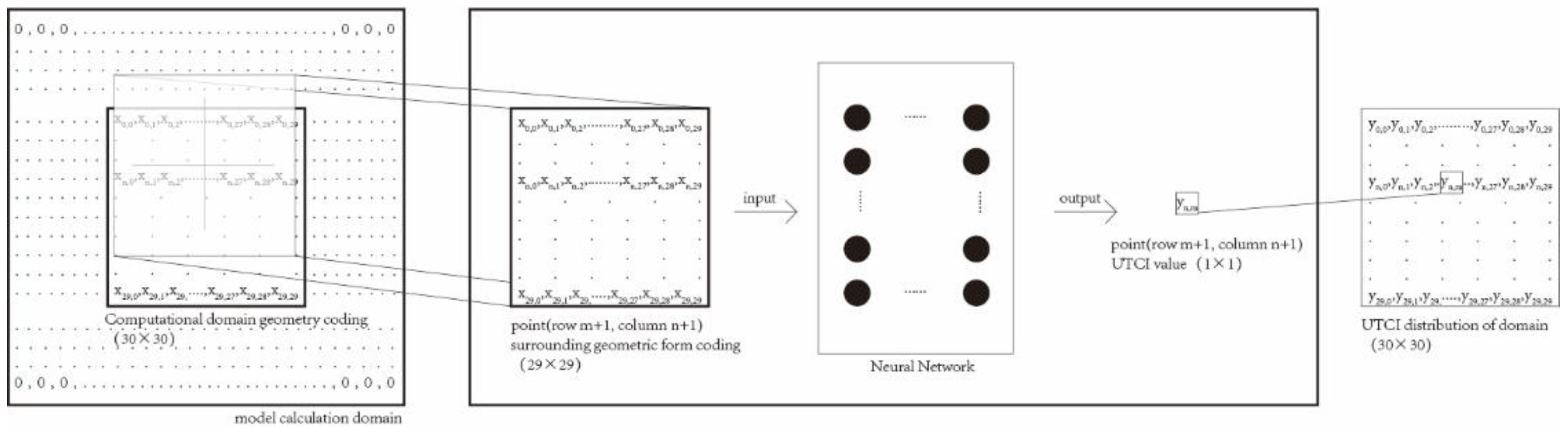
Group A regarded the block space as a whole, and the input of the model was the block space form coding, Si, with dimensions of 30 × 30. The output was the UTCI distribution of the pedestrian height plane, Ri, which had the same dimensions of 30 × 30. and from the Group A dataset (, ).
Group B regarded the block space as a discrete measurement point and calculations were made point-by-point based on the surrounding information of the measurement point. The input port of its model encodes the geometric block information in a specific range of surrounding blocks, denoted as , and the dimension was 29 × 29. The model’s output was the UTCI value of the point, which was recorded as , and the dimension was 1.
Both and were transformed from the original , as shown in Figure 7. Specifically, for the ith site case, the matrix corresponding to a point in the space of row m and column n in should be a 29 × 29 matrix consisting of to . The data corresponding to were the values in row m and column n of . After data rule conversion, each building site case could be converted into 900 sets of data, and a total of 1,749,539 pieces of data were obtained after removing duplicate data, forming the Group B dataset ().
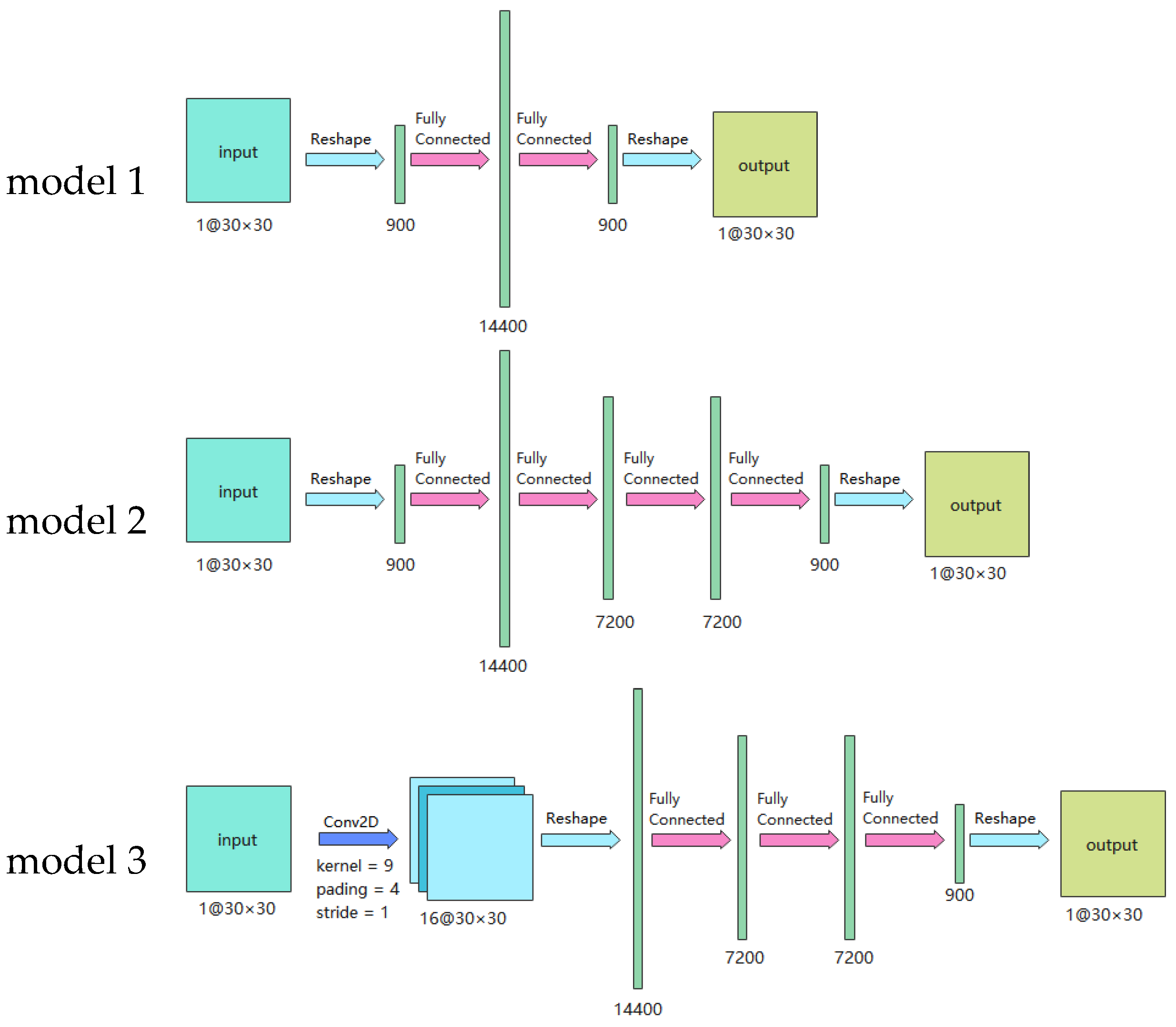
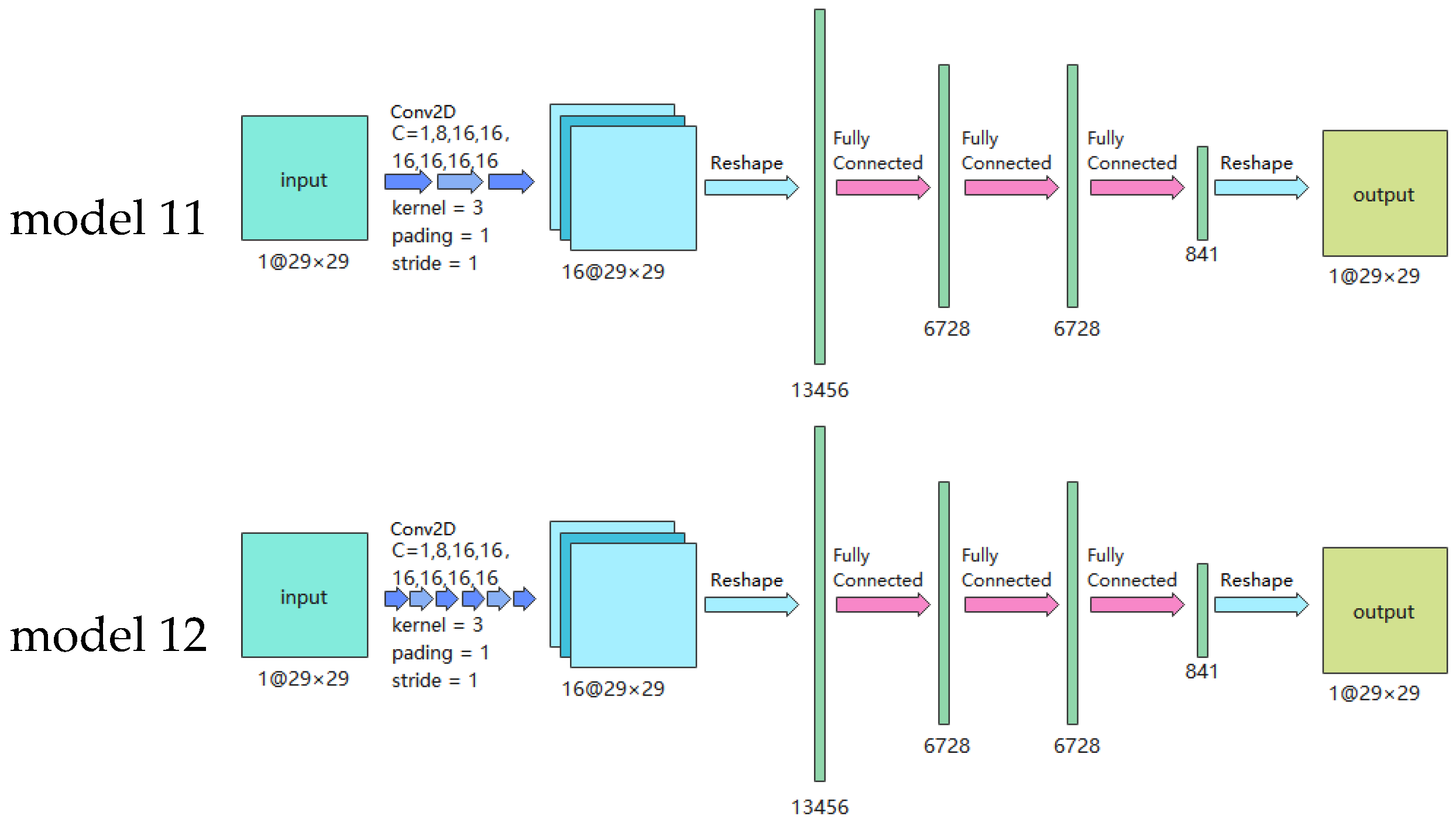
The role of the critical steps in a system can be judged and analyzed by adjusting the hyperparameters of models [28,29]. Therefore, for the two groups of models above, as shown in Table 4 and Table 5, different types of neural networks, different numbers of neural network layers, and different sizes of convolution kernel were separately used to construct neural network models, and each method formed six neural network models. Except for the different input and output layers, the other hidden layers of the two groups were set according to the same multiple and appeared in pairs. Specifically, models 1 and 7 were the benchmark models of the two groups, using one fully connected layer; models 2 and 8 had three fully connected layers; models 3, 4, 9, and 10, had one additional convolutional layer, with the convolution kernel matrix set as (3 × 3) and (9 × 9). Models 5, 6, 11, and 12 used three and six layers with 3 × 3 convolution kernels. After a series of settings, both groups of models had the same number of training parameters, as shown in Table 6 and Table 7. The neural network model structures are shown in Figure 8 and Figure 9. The generated code associated with the model can be downloaded from https://github.com/architsama/UTCI_distribution (accessed on 23 August 2022).
To ensure the consistency of the neural network training environment, all other parameters of each neural network model were uniformly set: the loss function used was the mean-square error (MSE), as shown in Equation (1). As the optimizer, I used Adam [51], the batch size for the training was 128, and the learning rate was 0.001. To facilitate comparison with other study results in the same field, I introduced a dimensionless index, the R2 score, to evaluate the degree of model regression effectiveness, as shown in Equation (2). Its value is usually between 0 and 1, where the closer the value to 1, the more accurately the model fits the data. I also introduced the index root-mean-squared error (RMSE) to facilitate lateral comparisons of model accuracy.
where is the output predicted by each model; is the average value of the calculation; is the value of the calculation; m is the number of cases in the dataset.
A computer equipped with AMD Ryzen 7 4800H CPU and NVIDIA GeForce RTX 2060 GPU was used to complete the training of 12 kinds of neural networks under the above two frameworks of Groups A and B. The neural network was implemented using the Python 3.7 programming language and the machine learning framework Pytorch. The cumulative running time of all model training was approximately 120 h.
3. Results and Discussion
In this section, I evaluate and compare the performance of each neural network on the training and test sets and visualize the internal hidden layers of the convolutional neural network to reveal the impact of different neural network architectures on the prediction performance.
3.1. Overall Situation of Two Groups of Network Training
To more intuitively represent the model training process, Figure 10 shows the performance of each model in each training epoch on the training and test sets, where the blue and red lines indicate the performance of each epoch on the training and testing sets, respectively. I trained the Group A models for 2500 generations and the Group B models for 300 generations. As can be observed in the figure, compared with the Group A model, the convergence speed of Group B was remarkably faster. Despite the larger number of training generations for the Group A models compared with the Group B model, Table 8 and Table 9 show that the loss function values of Group B were lower than those of Group A on both the test and training sets.
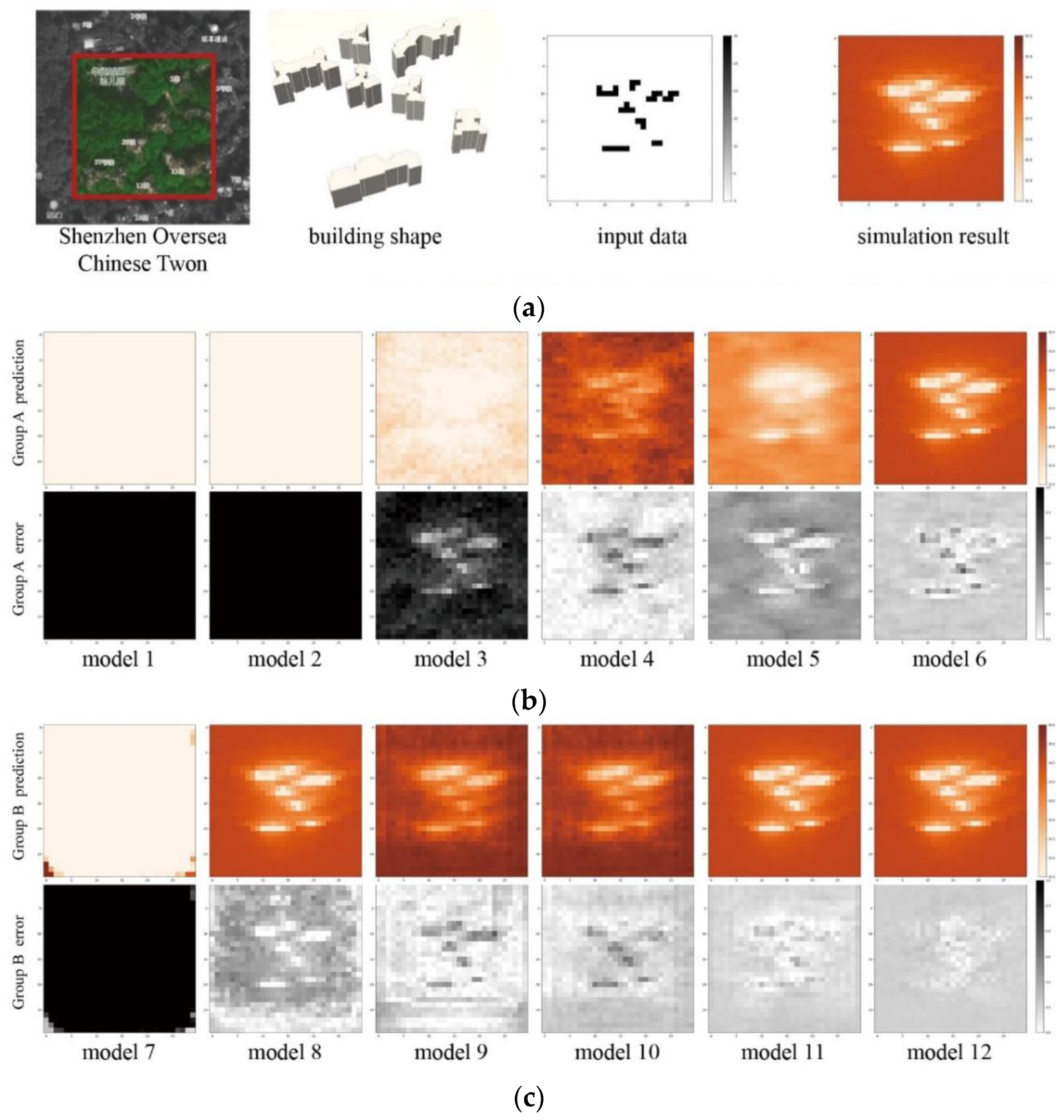
To further test the model’s prediction performance after training, I selected a residential group in Shenzhen Overseas Chinese Town, which was not included in the aforementioned dataset. Figure 11 shows each model group’s prediction and error distribution for this case, and I plotted the prediction and error charts separately using the same scales. From the models, on the whole, it can be seen that the Group B models outperformed those of Group A.
In this study, both groups used the same original datasets with similar neural network frameworks, but I found that the performance of the Group B models was overall better than that of the Group A models, which may have been related to the actual number of samples in the training dataset. Due to the change in the Group B model settings, the study object was transformed from site to measurement point, and the amount of data increased from 2400 to 1,749,539. This technique of artificially expanding the size of a training set by creating modified data from the existing data is known as data augmentation [52], which can be used to regularize systems and prevent overfitting in machine learning. Basic data augmentation can considerably improve accuracy on image tasks, such as classification and segmentation. Commonly used methods, including image synthesis operations such as flipping, erasing, and mirroring for image data, or using a generative adversarial network method to generate virtual data, can produce a larger dataset to enhance the training of the model.
Based on a reasonable inference of the theory, the Group B models transformed the perspective of space as a whole as an object into that of measuring points, thus increasing the amount of data and improving the model performance, which is a particular embodiment of the data augmentation theory in environmental performance prediction. Comparably, this space-to-point data enhancement method may also be applied in other scenarios of outdoor environmental performance prediction, such as wind environment prediction problems, sunshine hour calculation problems, etc.
3.2. Horizontal Comparison of Neural Network Model Performance
The convergence plots of the models of Group A in Figure 10 show that the convergence rate gradually increased from model 1 to 6. All models eventually converged at the 2500 epoch model. Table 8 shows that only model 6 performed well in all performance indicators, and that its R2 score was 0.927 on the test datasets, while the loss function was 0.022 on the test datasets, which demonstrated that the model had a stronger generalization ability. The performance on the test case of the Group A models in Figure 11 also verified the previous point. Among the six models, only the prediction diagram of model 6 could clearly distinguish the change in UTCI distribution caused by the shadow of the building on the site, and models 4 and 5 could barely capture the range of building influence, and the prediction effect of model 5 was slightly more accurate than that of model 4. The results predicted by models 1–3 were far from the actual results, as the errors mostly exceeded the threshold values.
Likewise, the individual models in Group B expressed similar trends. Figure 10 shows that the convergence speed of the Group B models from models 7 to 12 gradually increased, and finally, the models converged after 300 epochs. Table 9 shows that all performance indicators of models 8, 10, 11, and 12 performed well, with R2 scores between 0.814 and 0.960, as well as MSEs between 0.012 and 0.032 on the test datasets. I found that these models were able to accurately predict the UTCI for the site.
In the test cases, the prediction plots of the Group B models in Figure 11 are consistent with the calculated plots, except for those of model 7. The error of models 8 to 12 gradually decreased.
Based on the similar trends exhibited by the two groups of models, (1) for the artificial neural networks, models 2 and 8 performed better than models 1 and 7 on both the test and training sets in terms of all metrics, but the R2 score on the test set remained low. This may be due to the increase in the number of fully connected layers enhancing the model fitting effect to some extent. (2) The addition of convolutional layers substantially improved the prediction accuracy of the model, and the number and size of convolutional layers had different effects on this process. The cases of models 3 and 4, and models 9 and 10 showed that the cases with fewer kernel convolutional layers achieved more accurate results in this study. Additionally, the cases of models 3, 5, and 6 and models 9, 11, and 12 showed that the increase in the number of convolutional layers considerably increased the prediction accuracy of the model. In both groups, the convolutional neural network with six layers (3 × 3) of convolutional kernels performed the best.
3.3. Hidden-State Visualizations for Convolutional Neural Network
As described in the above results, convolutional neural networks performed better than artificial neural networks. Although the model fitting ability of the artificial neural networks was better on the training datasets, they lacked generalization ability on the test datasets, which may have been due to the parsing ability of the convolutional neural networks for morphological data, enabling the extraction of features related to the physical environment. However, in the neural network’s iterative training process, these learned features are challenging to identify and explain from the perspective of human vision. Hidden-state visualization technology can be used in convolutional neural networks to convert interior features into visually perceptible patterns [31,53] with the purpose of analyzing the analytical process of the neural network model for environmental performance simulation.
I chose model 6 as an example, randomly selected a case from the test dataset, and visualized the matrix data of channels 1–8 of all convolution layers, as shown in Figure 11. All figures are plotted with the same ruler, where the color depth represents the value, and the darker the color, the higher the value. Figure 12 shows that some spatial features in the input site were gradually labeled out as the number of convolution layers increased. I selected the calculation results of the first and last convolutional layer for comparison with the data input matrix, model prediction data, and calculated values, separately, as shown in Figure 13. In the figure, the first convolutional layer of the model only distinguishes the main body of the building from the surrounding site and labels the main body of the building according to some orientation rules. The last convolutional layer of the model provides some labels for the shadow areas around the building, and the image presents a shape closer to the final prediction. The number of parameters occupied by the convolutional layers in this process was only 0.0078% of the overall model data volume.
A convolutional neural network is a kind of neural network with typical spatial translation invariance [54], which may be one of the reasons why convolutional neural networks outperformed artificial neural networks in this study. For translation invariance, various hypotheses have been proposed for the mechanism of this property [55,56], one of which argues that translation invariance is determined by the increase in the receptive field size of the neurons in continuous convolutional layers. Because the convolutional kernel keeps the parameters shared globally in the participating convolutional computation, the constant invariance property in space can be refined. The neural network architecture in this study was built on the close relationship between the performance of the built environment and the building morphology, which is constant and does not change under a certain state due to the change in spatial location. In the processes of these calculations, the convolutional neural network may use the convolutional kernel as a medium to extract the spatial features of the site and resolve the spatial morphology of the site in a multilayer convolutional operation, which is followed by a fully connected layer to build a regression model between the features and performance, thus increasing the accuracy of the prediction results, as shown in Figure 14.
4. Conclusions and Future Work
4.1. Study Findings
In this study, I investigated the prediction of UTCI distribution by neural network models. The models were built on the a priori knowledge of the discipline and physical laws, and two different types of neural network models, Groups A and B, were constructed from the perspective of the environment as a whole and a point in space, respectively. Both models used the same size of substantive cases, but the models in Group B had an exponentially larger number of training sets after data transformation due to the different data structures. From the prediction results, benefiting from this theory-based data augmentation technique, Group B models produced more accurate predictions and showed higher generalization ability. The best-performing model was model 12, which had an MSE of 0.022 and an R2 score of 0.960 on the test set.
In the two groups, I constructed six neural networks with different numbers of layers, convolutional kernel sizes, and convolutional kernel layers. Comparing the performance of these models, I found that (1) all the models had some prediction accuracy on the training set, but the generalization ability of the artificial neural networks was weak. (2) For the artificial neural networks, an increase in the number of fully connected layers further increased their fitting effect on the training datasets, but the improvement on the test datasets was not apparent. (3) For the convolutional neural networks, the appropriate convolutional layer size and stack of appropriate convolutional layers considerably improved the model.
As stated above, the reason for these findings may have been that the spatial invariance of the convolution calculation allowed the most essential spatial features of the spatial environment to be captured. The regression function between the feature and predicted value did not change because of spatial changes, which eliminated the computational noise caused by spatial changes. In other words, although the study object was the UTCI distribution problem of the site, the convolutional neural network also played a role in establishing the same spatial morphological characteristics and environmental performance problems.
Finally, an internal hidden layer visualization analysis was performed for one set of convolutional neural network models, and I observed that the models were slowly extracted from their site space features during the iterative process of multilayer convolutional layers. Subsequently, the prediction of the models was achieved by establishing the regression between the space and performance results through the fully connected layers.
4.2. Limitations and Future Work
In this study, I built two types of neural network models with different architectures based on a priori knowledge through a hybrid-driven approach, using the UTCI computational problem as an example. Moreover, the running mechanism of convolutional neural networks when dealing with thus outdoor performance analysis problem was initially described through comparative experiments. However, future work can be conducted to address the following limitations:
- Although the study object was the UTCI distribution of the site, similarly, for outdoor wind environment prediction, building site insolation, outdoor thermal environment, and other problems are based on the constant law between certain spatial morphological characteristics and the performance of the built environment, I consider that the space analysis → data regression structure mentioned in this paper is also applicable.
- As mentioned in Section 2.1, I used the unit decomposition method for building analysis. Owing to the length of the article, I adopted one of the more simplified pseudo-2.5D parsing methods divided by the unit matrix, which converts 3D forms into 2D matrices with matrix cells of 10 × 10 × 1 m. Although overly large data dimensions were avoided to a certain extent, information density was also compromised, so an accuracy that is acceptable in actual architectural design problems was not attained. In following studies, the modeling accuracy can be further improved by combining the method with the actual requirements or using more accurate expressions such as point clouds and octrees.
- This study focused more on mechanism research and feasibility discussion. Compared with traditional simulation methods based on physical principles, machine learning computation is several orders of magnitude faster. The following studies can consider the requirements of building environmental performance problems, gradually consider more factors, introduce more cutting-edge neural network research results as a backbone, and build a practical machine learning simulation tool.
- The machine learning training process needs to provide a large amount of effective data. The data used in this study were obtained through software simulation. In this process, the accuracy of the simulation software directly limited the accuracy of the machine learning model. Unfortunately, temporarily completing the measurement during the completion of this study was not possible, but this defect will be addressed in a subsequent study. I will obtain valid data from monitoring stations or mobile measurements to complete the prediction of real physical environments.
Funding
This research received no external funding.
Institutional Review Board Statement
Not applicable.
Informed Consent Statement
Informed consent was obtained from all the subjects involved in the study.
Data Availability Statement
The supporting information can be downloaded at: https://github.com/architsama/UTCI_distribution (accessed on 23 August 2022). For raw data radar files, contact 2050321007@email.szu.edu.cn.
Conflicts of Interest
The author declares no conflict of interest.
References
- Huang, C.; Zhang, G.; Zhang, X.; Ying, M. Energy-driven urban intelligence Generation: Optimization of regional energy consumption in the early stage of design. Archit. Ski. 2021, 27, 78–83. [Google Scholar]
- Bogenstätter, U. Prediction and Optimization of Life-Cycle Costs in Early Design. Build. Res. Inf. 2000, 28, 376–386. [Google Scholar] [CrossRef]
- Purup, P.B.; Petersen, S. Requirement Analysis for Building Performance Simulation Tools Conformed to Fit Design Practice. Autom. Constr. 2020, 116, 103226. [Google Scholar] [CrossRef]
- Winkler, D.A.; Le, T.C. Performance of Deep and Shallow Neural Networks, the Universal Approximation Theorem, Activity Cliffs, and QSAR. Mol. Inf. 2017, 36, 1600118. [Google Scholar] [CrossRef] [Green Version]
- Manita, O.A.; Peletier, M.A.; Portegies, J.W.; Sanders, J.; Senen-Cerda, A. Universal Approximation in Dropout Neural Networks. J. Mach. Learn. Res. 2022, 23, 1–46. [Google Scholar]
- Kazanasmaz, T.; Günaydin, M.; Binol, S. Artificial Neural Networks to Predict Daylight Illuminance in Office Buildings. Build. Environ. 2009, 44, 1751–1757. [Google Scholar] [CrossRef] [Green Version]
- Paterson, G.H. Real-Time Environmental Feedback at the Early Design Stages. In Proceedings of the Computation and Performance—The 31st eCAADe Conference, Delft, The Netherlands, 18–20 September 2013; CUMINCAD. Stouffs, R., Sariyildiz, S., Eds.; Faculty of Architecture, Delft University of Technology: Delft, The Netherlands, 2013; 2, pp. 79–86. [Google Scholar]
- Jiaxin, Z. Sensitivity Analysis of Thermal Performance of Granary Building Based on Machine Learning. In Proceedings of the Intelligent & Informed—The 24th CAADRIA Conference, Wellington, New Zealand, 15–18 April 2019; CUMINCAD. Haeusler, M., Schnabel, M.A., Fukuda, T., Eds.; Victoria University of Wellington: Wellington, New Zealand, 2019; 1, pp. 665–674. [Google Scholar]
- Mokhtar, S.; Sojka, A.; Davila, C.C. Conditional Generative Adversarial Networks for Pedestrian Wind Flow Approximation. In Proceedings of the 11th Annual Symposium on Simulation for Architecture and Urban Design, Austria, Vienna, 25–27 May 2020; Society for Computer Simulation International: San Diego, CA, USA, 2020; p. 8. [Google Scholar]
- Duering, S.; Chronis, A.; Koenig, R. Optimsizing Urban Systems: Integrated Optimization of Spatial Configurations. In Proceedings of the 11th Annual Symposium on Simulation for Architecture and Urban Design, Austria, Vienna, 25–27 May 2020; Society for Computer Simulation International: San Diego, CA, USA, 2020; p. 7. [Google Scholar]
- Zhou, Q.; Ooka, R. Influence of Data Preprocessing on Neural Network Performance for Reproducing CFD Simulations of Non-Isothermal Indoor Airflow Distribution. Energy Build. 2021, 230, 110525. [Google Scholar] [CrossRef]
- Van Gelder, L.; Das, P.; Janssen, H.; Roels, S. Comparative Study of Metamodelling Techniques in Building Energy Simulation: Guidelines for Practitioners. Simul. Model. Pract. Theory 2014, 49, 245–257. [Google Scholar] [CrossRef]
- Zaghloul, M. Machine-Learning Aided Architectural Design-Synthesize Fast CFD by Machine-Learning; ETH Zurich: Zurich, Switzerland, 2017. [Google Scholar]
- Nault, E.; Moonen, P.; Rey, E.; Andersen, M. Predictive Models for Assessing the Passive Solar and Daylight Potential of Neighborhood Designs: A Comparative Proof-of-Concept Study. Build. Environ. 2017, 116, 1–16. [Google Scholar] [CrossRef] [Green Version]
- Østergård, T.; Jensen, R.L.; Maagaard, S.E. A Comparison of Six Metamodeling Techniques Applied to Building Performance Simulations. Appl. Energy 2018, 211, 89–103. [Google Scholar] [CrossRef]
- Fairbrass, A.J.; Firman, M.; Williams, C.; Brostow, G.J.; Titheridge, H.; Jones, K.E. CityNet—Deep Learning Tools for Urban Ecoacoustic Assessment. Methods Ecol. Evol. 2019, 10, 186–197. [Google Scholar] [CrossRef] [Green Version]
- Lorenz, C.-L.B.D.S. Machine Learning in Design Exploration: An Investigation of the Sensitivities of ANN-Based Daylight Predictions. In “Hello, Culture!”, Proceedings of the 18th International Conference, CAAD Futures 2019, Daejeon, Korea; CUMINCAD; Lee, J.-H., Ed.; Springer: Berlin/Heidelberg, Germany, 2019; pp. 75–87. ISBN 978-89-89453-05-5. [Google Scholar]
- Sebestyen, A.; Tyc, J. Machine Learning Methods in Energy Simulations for Architects and Designers. In Proceedings of the of the 38th eCAADe Conference, Berlin, Germany, 16–18 September 2020; p. 10. [Google Scholar]
- Shen, L.; Han, Y. Comparative Analysis of Machine Learning Models Optimized by Bayesian Algorithm for Indoor Daylight Distribution Prediction. In Proceedings of the 5th PLEA Conference on Passive and Low Energy Architecture, A Coruña, Spain, 1–3 September 2020; Universidade da Coruña: Coruña, Spain, 2020. [Google Scholar]
- Zhou, Q.; Ooka, R. Comparison of Different Deep Neural Network Architectures for Isothermal Indoor Airflow Prediction. Build. Simul. 2020, 13, 1409–1423. [Google Scholar] [CrossRef]
- Isola, P.; Zhu, J.-Y.; Zhou, T.; Efros, A.A. Image-to-Image Translation with Conditional Adversarial Networks. In Proceedings of the IEEE Conference on Computer Vision and Pattern Recognition (CVPR), Honolulu, HI, USA, 21–26 July 2017. [Google Scholar]
- Jendritzky, G.; de Dear, R.; Havenith, G. UTCI—Why Another Thermal Index? Int. J. Biometeorol. 2012, 56, 421–428. [Google Scholar] [CrossRef] [PubMed] [Green Version]
- Blazejczyk, K.; Epstein, Y.; Jendritzky, G.; Staiger, H.; Tinz, B. Comparison of UTCI to Selected Thermal Indices. Int. J. Biometeorol. 2012, 56, 515–535. [Google Scholar] [CrossRef] [Green Version]
- Maass, W.; Parsons, J.; Purao, S.; Storey, V.; Woo, C. Data-Driven Meets Theory-Driven Research in the Era of Big Data: Opportunities and Challenges for Information Systems Research. J. Assoc. Inf. Syst. 2018, 19, 1253–1273. [Google Scholar] [CrossRef] [Green Version]
- Reichstein, M.; Camps-Valls, G.; Stevens, B.; Jung, M.; Denzler, J.; Carvalhais, N. Prabhat Deep Learning and Process Understanding for Data-Driven Earth System Science. Nature 2019, 566, 195–204. [Google Scholar] [CrossRef]
- Kucikova, L.; Danso, S.; Jia, L.; Su, L. Computational Psychiatry and Computational Neurology: Seeking for Mechanistic Modeling in Cognitive Impairment and Dementia. Front. Comput. Neurosci. 2022, 16, 1–5. [Google Scholar] [CrossRef]
- Gan, V.J.L.; Wang, B.; Chan, C.M.; Weerasuriya, A.U.; Cheng, J.C.P. Physics-Based, Data-Driven Approach for Predicting Natural Ventilation of Residential High-Rise Buildings. Build. Simul. 2022, 15, 129–148. [Google Scholar] [CrossRef]
- Cheng, K.; Wang, N.; Shi, W.; Zhan, Y. Research progress on interpretability of deep learning. Comput. Res. Dev. 2020, 57, 1208–1217. [Google Scholar]
- Lei, X.; Luo, X. A survey of deep learning interpretability. Appl. Comput. 2022, 1–17. [Google Scholar]
- Wei, X. Visual Analysis of Fine-Grained Images Based on Deep Learning. Ph.D. Thesis, Nanjing University, Nanjing, China, 2018. [Google Scholar]
- Wang, Z.J.; Turko, R.; Shaikh, O.; Park, H.; Das, N.; Hohman, F.; Kahng, M.; Chau, D.H. CNN Explainer: Learning Convolutional Neural Networks with Interactive Visualization. IEEE Trans. Vis. Comput. Graph. 2020, 27, 1396–1406. [Google Scholar] [CrossRef] [PubMed]
- Liu, Y.; Lu, Y.; Wang, Y.; Sun, D.; Deng, L.; Wang, F.; Lei, Y. A CNN-Based Shock Detection Method in Flow Visualization. Comput. Fluids 2019, 184, 1–9. [Google Scholar] [CrossRef]
- Yi, T.B.L. CNN-Based Flow Field Feature Visualization Method. Int. J. Perform. Eng. 2018, 14, 434. [Google Scholar] [CrossRef]
- Arun, N.; Gaw, N.; Singh, P.; Chang, K.; Aggarwal, M.; Chen, B.; Hoebel, K.; Gupta, S.; Patel, J.; Gidwani, M.; et al. Assessing the Trustworthiness of Saliency Maps for Localizing Abnormalities in Medical Imaging. Radiol. Artif. Intell. 2021, 3, e200267. [Google Scholar] [CrossRef] [PubMed]
- Garg, S.; Garg, S. Prediction of Lung and Colon Cancer through Analysis of Histopathological Images by Utilizing Pre-Trained CNN Models with Visualization of Class Activation and Saliency Maps. In Proceedings of the 2020 3rd Artificial Intelligence and Cloud Computing Conference, Association for Computing Machinery, New York, NY, USA, 18 December 2020; pp. 38–45. [Google Scholar]
- Achour, Y.S.; Kharrat, F. Influence of Urban Morphology on Outdoor Thermal Comfort in Summer: A Study in Tunis, Tunisia. Mod. Environ. Sci. Eng. 2016, 2, 251–256. [Google Scholar] [CrossRef]
- Chen, Y.; Wang, Y.; Zhou, D. Knowledge Map of Urban Morphology and Thermal Comfort: A Bibliometric Analysis Based on CiteSpace. Buildings 2021, 11, 427. [Google Scholar] [CrossRef]
- Xu, X.; Yin, C.; Wang, W.; Xu, N.; Hong, T.; Li, Q. Revealing Urban Morphology and Outdoor Comfort through Genetic Algorithm-Driven Urban Block Design in Dry and Hot Regions of China. Sustainability 2019, 11, 3683. [Google Scholar] [CrossRef] [Green Version]
- Requicha, A.G. Representations for Rigid Solids: Theory, Methods, and Systems. ACM Comput. Surv. 1980, 12, 437–464. [Google Scholar] [CrossRef]
- Roman, N.D.; Bre, F.; Fachinotti, V.D.; Lamberts, R. Application and Characterization of Metamodels Based on Artificial Neural Networks for Building Performance Simulation: A Systematic Review. Energy Build. 2020, 217, 109972. [Google Scholar] [CrossRef]
- Han, Y.; Shen, L.; Sun, C. Developing a Parametric Morphable Annual Daylight Prediction Model with Improved Generalization Capability for the Early Stages of Office Building Design. Build. Environ. 2021, 200, 107932. [Google Scholar] [CrossRef]
- Han, Z.; Yan, W.; Liu, G. A Performance-Based Urban Block Generative Design Using Deep Reinforcement Learning and Computer Vision. In Proceedings of the 2020 Digital Futures, online, 12–15 October 2020; Yuan, P.F., Yao, J., Yan, C., Wang, X., Leach, N., Eds.; Springer: Singapore, 2021; pp. 134–143. [Google Scholar] [CrossRef]
- Zhu, S.; Ma, C.; Zhang, Y.; Xiang, K. A Hybrid Metamodel-Based Method for Quick Energy Prediction in the Early Design Stage. J. Clean. Prod. 2021, 320, 128825. [Google Scholar] [CrossRef]
- Jendritzky, G.; Havenith, G.; Weihs, P.; Batchvarova, E. COST Action 730 on the Universal Thermal Climate Index UTCI. In Proceedings of the 17th International Congress Biometeorology ICB, Garmisch-Partenkirchen, Germany, 17 April 2006; pp. 309–312. [Google Scholar]
- Jendritzky, G.; Maarouf, A.; Fiala, D.; Staiger, H. An Update on the Development of a Universal Thermal Climate Index. In Proceedings of the 15th Conference on Biometeorology/Aerobiology and 16th International Congress of Biometeorology, Kansas City, MO, USA, 27 October–1 November 2002; pp. 129–133. [Google Scholar]
- Fiala, D.; Havenith, G.; Bröde, P.; Kampmann, B.; Jendritzky, G. UTCI-Fiala Multi-Node Model of Human Heat Transfer and Temperature Regulation. Int. J. Biometeorol. 2012, 56, 429–441. [Google Scholar] [CrossRef] [PubMed] [Green Version]
- Bröde, P.; Fiala, D.; Błażejczyk, K.; Holmér, I.; Jendritzky, G.; Kampmann, B.; Tinz, B.; Havenith, G. Deriving the Operational Procedure for the Universal Thermal Climate Index (UTCI). Int. J. Biometeorol. 2012, 56, 481–494. [Google Scholar] [CrossRef]
- Arens, E.; Hoyt, T.; Zhou, X.; Huang, L.; Zhang, H.; Schiavon, S. Modeling the Comfort Effects of Short-Wave Solar Radiation Indoors. Build. Environ. 2015, 88, 3–9. [Google Scholar] [CrossRef] [Green Version]
- Ibrahim, Y.; Kershaw, T.; Shepherd, P.; Elwy, I. A Parametric Optimisation Study of Urban Geometry Design to Assess Outdoor Thermal Comfort. Sust. Cities Soc. 2021, 75, 103352. [Google Scholar] [CrossRef]
- Xue, P.; Li, Q.; Xie, J.; Zhao, M.; Liu, J. Optimization of Window-to-Wall Ratio with Sunshades in China Low Latitude Region Considering Daylighting and Energy Saving Requirements. Appl. Energy 2019, 233–234, 62–70. [Google Scholar] [CrossRef]
- Kingma, D.P.; Ba, J. Adam: A Method for Stochastic Optimization. arXiv 2014, arXiv:1412.6980. [Google Scholar] [CrossRef]
- Yang, S.; Xiao, W.; Zhang, M.; Guo, S.; Zhao, J.; Shen, F. Image Data Augmentation for Deep Learning: A Survey. arXiv 2022, arXiv:2204.08610. [Google Scholar]
- Qin, Z.; Yu, F.; Liu, C.; Chen, X. How Convolutional Neural Network See the World—A Survey of Convolutional Neural Network Visualization Methods. Math. Found. Comput. 2018, 1, 149–180. [Google Scholar] [CrossRef]
- Ruderman, A.; Rabinowitz, N.C.; Morcos, A.S.; Zoran, D. Pooling Is Neither Necessary nor Sufficient for Appropriate Deformation Stability in CNNs. arXiv 2018, arXiv:1804.04438. [Google Scholar]
- Kauderer-Abrams, E. Quantifying Translation-Invariance in Convolutional Neural Networks. arXiv 2017, arXiv:1801.01450. [Google Scholar]
- Kayhan, O.S.; van Gemert, J.C. On Translation Invariance in CNNs: Convolutional Layers Can Exploit Absolute Spatial Location. In Proceedings of the IEEE/CVF Conference on Computer Vision and Pattern Recognition (CVPR), Seattle, WA, USA, 13–19 June 2020; pp. 14274–14285. [Google Scholar]
Figure 1.
(a) Theory-driven, (b) data-driven [26], and (c) hybrid-driven paradigms.
Figure 1.
(a) Theory-driven, (b) data-driven [26], and (c) hybrid-driven paradigms.

Figure 2.
Neural network training process.

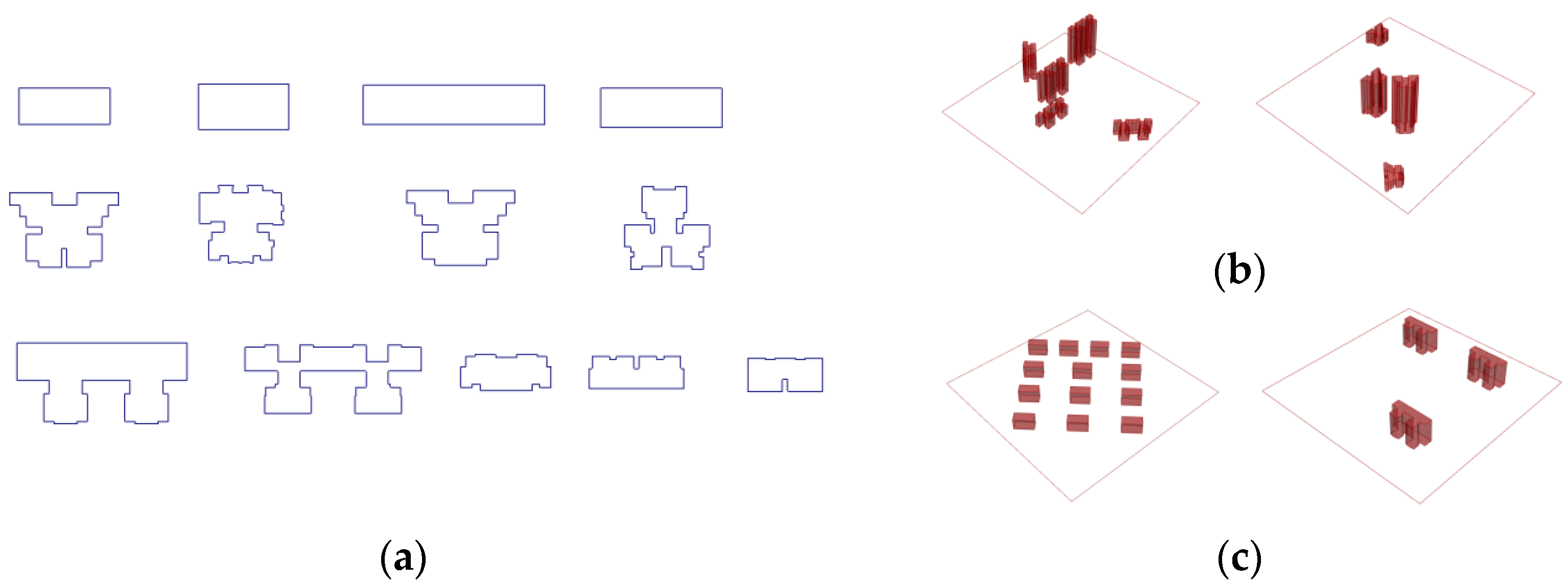
Figure 3.
Architectural form generation case schematic: (a) 13 commonly used residential building contours; (b) first residential area form with free layout; (c) second architectural form with determinant layout.
Figure 3.
Architectural form generation case schematic: (a) 13 commonly used residential building contours; (b) first residential area form with free layout; (c) second architectural form with determinant layout.

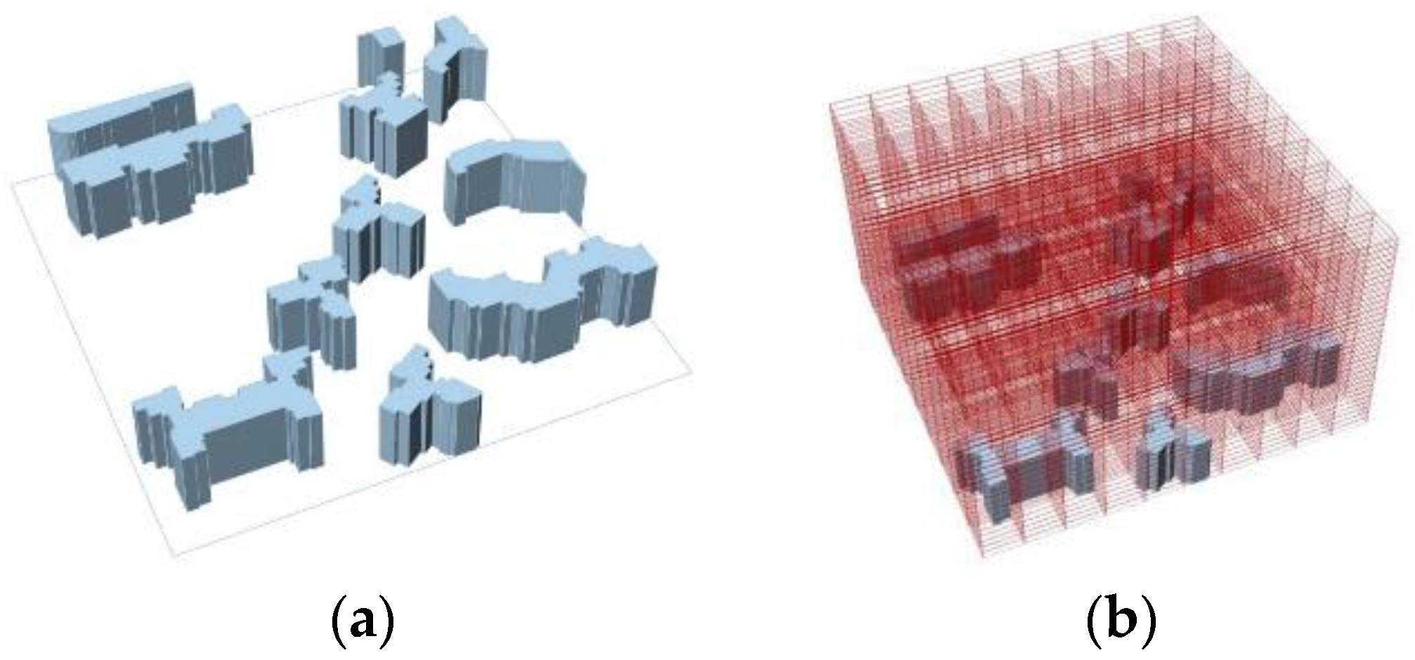
Figure 4.
Building dataset generation process: (a) original building case, (b) orthogonal network is used to determine the architectural form and convert it into a 2D matrix, (c) transform the 2D matrix into 3D, and (d) UTCI distribution of the site is calculated using the recoded form and converted into a 2D matrix.


Figure 5.
Schematic diagram of Group A.

Figure 6.
Schematic diagram of Group B.

Figure 7.
Data conversion rules in Group B dataset.

Figure 8.
Diagram of each neural network model structure in Group A.


Figure 9.
Diagram of each neural network model structure in Group B.


Figure 10.
Calculation of each model (epoch R2 score).

Figure 11.
Prediction results of each model for test cases. (a) UTCI calculation for a real project; (b) 6 Group A and (c) 6 Group B models’ prediction values and errors.
Figure 11.
Prediction results of each model for test cases. (a) UTCI calculation for a real project; (b) 6 Group A and (c) 6 Group B models’ prediction values and errors.

Figure 12.
Visualization of convolutional layers.

Figure 13.
Comparison between typical hidden layer and calculation process of a random case in test dataset: (a) input matrix, (b) calculation data of convolution layer 1, (c) calculation data of convolution layer 6, (d) final prediction data, and (e) value calculated by Ladybug.
Figure 13.
Comparison between typical hidden layer and calculation process of a random case in test dataset: (a) input matrix, (b) calculation data of convolution layer 1, (c) calculation data of convolution layer 6, (d) final prediction data, and (e) value calculated by Ladybug.

Figure 14.
Schematic diagram of neural network prediction principle.


Table 1.
Summary table of studies on building physical environment related to neural networks.
| NO. | Author(s), Year | Methods | Object of Study |
|---|---|---|---|
| 1 | Kazanasmaz et al., 2009 [6] | ANN * | Indoor daylight simulation |
| 2 | Paterson, 2013 [7] | ANN | Energy consumption |
| 3 | Van Gelder et al., 2014 [12] | RF * | Energy consumption |
| 4 | Zaghloul, 2017 [13] | SOM * | Outdoor wind environment |
| 5 | Nault et al., 2017 [14] | ANN | Energy consumption |
| 6 | Østergård et al., 2018 [15] | ANN | Energy consumption |
| 7 | Jiaxin, 2019 [8] | ANN | Energy consumption |
| 8 | Fairbrass et al., 2019 [16] | CNN * | Outdoor sound environment |
| 9 | Lorenz, 2019 [17] | ANN | Sunlight simulation |
| 10 | Sebestyen and Tyc, 2019 [18] | CNN | Sunlight simulation |
| 11 | SHEN and HAN, 2020 [19] | XGB *, RF, SVR * | Indoor daylight simulation |
| 12 | Zhou and Ooka, 2021 [11] | ANN | Indoor wind environment |
| 13 | Zhou and Ooka, 2020 [20] | ANN | Indoor wind environment |
| 14 | Mokhtar et al., 2020 [9] | PIX2PIX * | Outdoor wind environment |
| 15 | Duering et al., 2020 [10] | PIX2PIX | Outdoor wind environment |
* ANN, artificial neural network; RF, random forest; SOM, self-organizing map; CNN, convolutional neural network; XGB, extreme gradient boosting; SVR, support vector regression; PIX2PIX, conditional adversarial network of image-to-image translation [21].
Table 2.
Literature related to different forms of description methods in field of machine learning.
| Form Description Method | Research | Aim |
|---|---|---|
| Parameter representation | [6,8,13,19] | Indoor daylight simulation energy consumption |
| Constructive solid geometry | [12,14,15,40] | Energy consumption |
| Cell decomposition | [9,10,11,20] | Outdoor wind environment Indoor wind environment Sunlight simulation |
Table 3.
Software list.
| Software | Version |
|---|---|
| rhino | version 6 SR30, 14 October 2020 |
| grasshopper | version 1.0.0007 14 October 2020 |
| honeybee | version 0.0.66 |
| ladybug | version 0.0.69 |
| radiance | version 5.2.1 |
Table 4.
Architecture of models in Group A.
| ANN | CNN | ||||||
|---|---|---|---|---|---|---|---|
| Model 1 | Model 2 | Model 3 | Model 4 | Model 5 | Model 6 | ||
| Input layer | [30 × 30] | [30 × 30] | [30 × 30] | [30 × 30] | [30 × 30] | [30 × 30] | |
| Reshape | [900] | [900] | -- | -- | -- | -- | |
| Conv2d | 1 | - | - | (1,16),9,1 | (1,16),3,4 | (1,8),3,1 | (1,8),3,1 |
| 2 | - | - | - | - | (8,16),3,1 | (8,16),3,1 | |
| 3 | - | - | - | - | (16,16),3,1 | (16,16),3,1 | |
| 4 | - | - | - | - | - | (16,16),3,1 | |
| 5 | - | - | - | - | - | (16,16),3,1 | |
| 6 | - | - | - | - | - | (16,16),3,1 | |
| FCL | 1 | 14,400 | 14,400 | 14,400 | 14,400 | 14,400 | 14,400 |
| 2 | - | 7200 | 7200 | 7200 | 7200 | 7200 | |
| 3 | - | 7200 | 7200 | 7200 | 7200 | 7200 | |
| output | [900] | [900] | [900] | [900] | [900] | [900] | |
Table 5.
Architecture of models in Group B.
| ANN | CNN | ||||||
|---|---|---|---|---|---|---|---|
| Model 1 | Model 2 | Model 3 | Model 4 | Model 5 | Model 6 | ||
| Input layer | [30 × 30] | [30 × 30] | [30 × 30] | [30 × 30] | [30 × 30] | [30 × 30] | |
| Reshape | [900] | [900] | -- | -- | -- | -- | |
| Conv2d * | 1 | - | - | (1,16),9,1 | (1,16),3,4 | (1,8),3,1 | (1,8),3,1 |
| 2 | - | - | - | - | (8,16),3,1 | (8,16),3,1 | |
| 3 | - | - | - | - | (16,16),3,1 | (16,16),3,1 | |
| 4 | - | - | - | - | - | (16,16),3,1 | |
| 5 | - | - | - | - | - | (16,16),3,1 | |
| 6 | - | - | - | - | - | (16,16),3,1 | |
| FCL | 1 | 14,400 | 14,400 | 14,400 | 14,400 | 14,400 | 14,400 |
| 2 | - | 7200 | 7200 | 7200 | 7200 | 7200 | |
| 3 | - | 7200 | 7200 | 7200 | 7200 | 7200 | |
| output | [900] | [900] | [900] | [900] | [900] | [900] | |
* In Conv2d, [(1,16),3,1] means the input channel is 1, the output channel is 16, the convolution kernel is (3,3), and the padding is (1,1).
Table 6.
Trainable parameters of Group A.
| Parameter | Model 1 | Model 2 | Model 3 | Model 4 | Model 5 | Model 6 |
|---|---|---|---|---|---|---|
| CNN | 0 | 0 | 160 | 1312 | 3568 | 10,528 |
| FCL | 48,627,900 | 174,989,700 | 162,015,300 | 162,015,300 | 162,015,300 | 162,015,300 |
| ALL | 48,627,900 | 174,989,700 | 162,015,460 | 162,016,612 | 162,018,868 | 162,025,828 |
Table 7.
Trainable parameters of Group B.
| Parameter | Model 7 | Model 8 | Model 9 | Model 10 | Model 11 | Model 12 |
|---|---|---|---|---|---|---|
| CNN | 0 | 0 | 160 | 1312 | 3568 | 10,528 |
| FCL | 11,343,409 | 147,148,089 | 135,818,137 | 135,818,137 | 135,818,137 | 135,818,137 |
| ALL | 11,343,409 | 147,148,089 | 135,818,297 | 135,819,449 | 135,821,705 | 135,828,665 |
Table 8.
Performance of Group A models at 2500 epochs.
| ANN | CNN | ||||||
|---|---|---|---|---|---|---|---|
| Model 1 | Model 2 | Model 3 | Model 4 | Model 5 | Model 6 | ||
| MSE | Training dataset | 0.111 | 0.084 | 0.163 | 0.030 | 0.009 | 0.021 |
| Testing dataset | 0.138 | 0.095 | 0.162 | 0.035 | 0.010 | 0.022 | |
| Difference | 0.027 | 0.011 | −0.001 | 0.005 | 0.001 | 0.001 | |
| RMSE | Training dataset | 0.333 | 0.290 | 0.404 | 0.173 | 0.095 | 0.145 |
| Testing dataset | 0.371 | 0.308 | 0.402 | 0.187 | 0.100 | 0.148 | |
| Difference | 0.038 | 0.018 | −0.001 | 0.014 | 0.005 | 0.003 | |
| R2 Score | Training dataset | 0.793 | 0.845 | 0.648 | 0.937 | 0.983 | 0.959 |
| Testing dataset | 0.010 | 0.020 | 0.003 | 0.158 | 0.259 | 0.927 | |
| Difference | 0.783 | 0.825 | 0.645 | 0.779 | 0.724 | 0.032 | |
Table 9.
Performance of Group B models at 300 epochs.
| ANN | CNN | ||||||
|---|---|---|---|---|---|---|---|
| Model 1 | Model 2 | Model 3 | Model 4 | Model 5 | Model 6 | ||
| MSE | Training dataset | 0.108 | 0.002 | 0.279 | 0.092 | 0.031 | 0.014 |
| Testing dataset | 0.25 | 0.012 | 0.297 | 0.127 | 0.032 | 0.022 | |
| Difference | 0.142 | 0.010 | 0.018 | 0.035 | 0.001 | 0.008 | |
| RMSE | Training dataset | 0.329 | 0.045 | 0.528 | 0.303 | 0.176 | 0.118 |
| Testing dataset | 0.500 | 0.110 | 0.545 | 0.356 | 0.179 | 0.148 | |
| Difference | 0.171 | 0.065 | 0.017 | 0.053 | 0.003 | 0.030 | |
| R2 Score | Training dataset | 0.676 | 0.979 | 0.354 | 0.83 | 0.952 | 0.977 |
| Testing dataset | −0.012 | 0.835 | 0.291 | 0.814 | 0.943 | 0.960 | |
| Difference | 0.688 | 0.144 | 0.063 | 0.016 | 0.009 | 0.017 | |
Publisher’s Note: MDPI stays neutral with regard to jurisdictional claims in published maps and institutional affiliations. |
© 2022 by the author. Licensee MDPI, Basel, Switzerland. This article is an open access article distributed under the terms and conditions of the Creative Commons Attribution (CC BY) license (https://creativecommons.org/licenses/by/4.0/).
Share and Cite
MDPI and ACS Style
Zhong, G. Convolutional Neural Network Model to Predict Outdoor Comfort UTCI Microclimate Map. Atmosphere 2022, 13, 1860. https://doi.org/10.3390/atmos13111860
AMA Style
Zhong G. Convolutional Neural Network Model to Predict Outdoor Comfort UTCI Microclimate Map. Atmosphere. 2022; 13(11):1860. https://doi.org/10.3390/atmos13111860
Chicago/Turabian StyleZhong, Guodong. 2022. "Convolutional Neural Network Model to Predict Outdoor Comfort UTCI Microclimate Map" Atmosphere 13, no. 11: 1860. https://doi.org/10.3390/atmos13111860
Note that from the first issue of 2016, this journal uses article numbers instead of page numbers. See further details here.