Article

Flooded Extent and Depth Analysis Using Optical and SAR Remote Sensing with Machine Learning Algorithms

by
Jesús Soria-Ruiz
1,
Yolanda M. Fernandez-Ordoñez
2,*,
Juan P. Ambrosio-Ambrosio
2,
Miguel J. Escalona-Maurice
3,
Guillermo Medina-García
4,
Erasto D. Sotelo-Ruiz
1 and
Martha E. Ramirez-Guzman
5
1
Geomatics Lab, National Institute of Research for Forestry Agricultural and Livestock (INIFAP), Zinacantepec 51350, Mexico
2
Computer Science, Postgraduate College in Agricultural Sciences (COLPOS), Texcoco 56100, Mexico
3
Rural Development Studies, COLPOS, Texcoco 56100, Mexico
4
Zacatecas Experimental Station-INIFAP, Calera 53250, Mexico
5
Statistics Program, COLPOS, Texcoco 56100, Mexico
*
Author to whom correspondence should be addressed.
Atmosphere 2022, 13(11), 1852; https://doi.org/10.3390/atmos13111852
Submission received: 30 September 2022 / Revised: 28 October 2022 / Accepted: 31 October 2022 / Published: 7 November 2022
(This article belongs to the Special Issue Natural Disasters and Hazards in the Geographical Environment)

Abstract

:
Recurrent flooding occurs in most years along different parts of the Gulf of Mexico coastline and the central and southeastern parts of Mexico. These events cause significant economic losses in the agricultural, livestock, and infrastructure sectors, and frequently involve loss of human life. Climate change has contributed to flooding events and their more frequent occurrence, even in areas where such events were previously rare. Satellite images have become valuable information sources to identify, precisely locate, and monitor flooding events. The machine learning models use remote sensing images pixels as input feature. In this paper, we report a study involving 16 combinations of Sentinel-1 SAR images, Sentinel-2 optical images, and digital elevation model (DEM) data, which were analyzed to evaluate the performance of two widely used machine learning algorithms, gradient boosting (GB) and random forest (RF), for providing information about flooding events. With machine learning models GB and RF, the input dataset (Sentinel-1, Sentinel-2, and DEM) was used to establish rules and classify the set in the categories specified by previous tags. Monitoring of flooding was performed by tracking the evolution of water bodies during the dry season (before the event) through to the occurrence of floods during the rainy season (during the event). For detection of bodies of water in the dry season, the metrics indicate that the best algorithm is GB with combination 15 (F1m = 0.997, AUC = 0.999, K = 0.994). In the rainy season, the GB algorithm had better metrics with combination 16 (F1m = 0.995, AUC = 0.999, Kappa = 0.994), and detected an extent of flooded areas of 1113.36 ha with depths of <1 m. The high classification performance shown by machine learning algorithms, particularly the so-called assembly algorithms, means that they should be considered capable of improving satellite image classification for detection of flooding over traditional methods, in turn leading to better monitoring of flooding at local, regional, and continental scales.

1. Introduction

The scale of recent changes across the climate system as a whole and the present state of many aspects of the climate system are unprecedented over many centuries to many thousands of years. The frequency of occurrence of extreme weather events is increasing in many parts of the planet. Rain events have increased in frequency and intensity since the 1950s over most of Earth’s surface, with the available observational data identifying trends in human-induced climate change as the main driver [1]. Climate change has innumerable impacts worldwide, which can be observed in terms of its repercussions on sea level rise, heat waves, storms, drought, floods, reduction of glaciers, economic instability, and the destruction of ecosystems, among others. Rain affects daily life in many ways, its distribution in space and time directly has repercussions on the availability of fresh water, which is vital for the sustenance of life [2]. Weather is an integral part of daily life and has enormous impact on the economy, public health, and safety in the worldwide. Extreme rain events causing flooding and triggering landslides have significant socioeconomic impacts on society [3,4]. In central and southeastern Mexico, floods occur as a result of the convergence of intertropical air masses that causes intense rainfall in a short period of time, with the natural drainage network being insufficient to cope with these high rainfall amounts, causing the overflow of rivers, lakes, and lagoons. Such flooding causes significant economic losses every year in the agricultural, livestock, and infrastructure sectors, in addition to directly affecting human lives and livelihoods. One of the important issues concerning flooding in both Mexico and other countries is the need for rapid assessment of damage on which basis mitigation strategies can be formulated and applied [5].
Satellite images have become widely used for monitoring flooding in various parts of the world. They allow wider extents and/or specific areas of flooding to be observed. In addition, satellite images are available in diverse spatial, temporal, and spectral resolutions, meaning that they can provide high-quality results and useful information. Synthetic aperture radar (SAR) can operate under a variety of meteorological conditions [6]. However, because of the way in which they are obtained, SAR images require careful processing prior to analysis [7].
The complexity of monitoring events using SAR images increases when studying tropical areas on account of the density and height of vegetation. The backscatter of waves emitted by the SAR sensor suffers distortions and double-bouncing effects caused by vegetation, which limits the detection of flooded areas. However, proposals have been made to improve the ability of the SAR method to obtain information of interest [8,9,10].
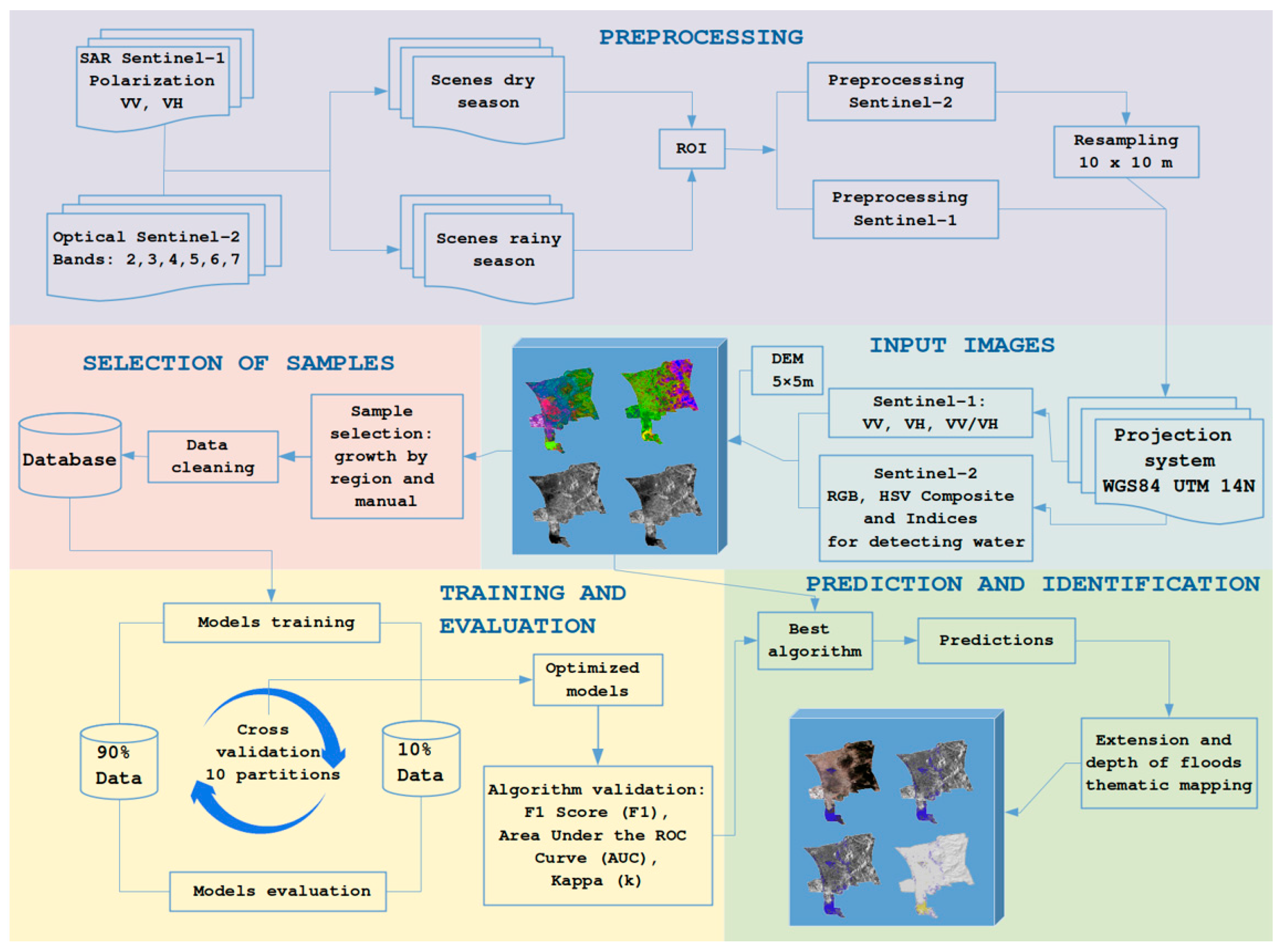
The use of optical multispectral satellite images and digital elevation models (DEMs) as complements to SAR images has the potential to increase the accuracy of classification based on the better spectral correlation between the optical sensors with their respective topographic and water-body information [11]. Combining these two types of image processing allows the extent and depth of flooding to be better detected, analyzed, and monitored [12,13,14].
DEMs are geospatial data of great importance in studies related to detection, monitoring, diagnosis, prediction and indirect estimation of depth of flood events [15,16]. DEMs are generated using different methods and technologies. Pure LIDAR data (raw data) have inherent errors due to obstacles and terrain conditions, which is why a set of cleaning procedures are usually applied [17,18]. Such procedures include interpolation techniques, which allowed us to obtain a DEM with a vertical and horizontal resolution of 5 m.
Timely information about floodwater depth is important for directing rescue and relief resources and determining road closures and accessibility. Once available, flood depth information can also be used for post-event analysis of property damage and flood-risk assessment. Several approaches for quantifying flood depth using remote sensing-based flood maps have been proposed; one of them is [19], who used “Floodwater Depth Estimation Tool (FwDET)”, developed to augment remote sensing analysis by calculating water depth based on an inundation map with an associated digital elevation model (DEM).
Furthermore, current computational power enables the implementation of machine-learning techniques for modeling multi-dimensional problems. In agriculture, these techniques have been used for estimating the height of crops, extent of irrigation, and extent and depth of flooding, as well as for identifying pests and diseases [20]. One of the key tasks in detecting flooding is classification, for which machine learning algorithms have shown superior performance to traditional binary segmentation methods [21].
Machine learning (ML) models based on decision trees can use the input dataset (Sentinel-1 SAR, Optical Sentinel-2, and DEM), to establish rules that allow it to classify the set into the categories specified by previous tags [11,17,22]. The algorithm selects the best attribute or characteristics (image pixels) and recursively partitions the labeled data until the following rule is met: all samples belong to the same attribute, there are no more samples, or there are no more features to perform the division [22]. The integration of remote sensing to ML algorithms has obtained a good performance in the detection water bodies [22,23]. One of the advantages of ML algorithms is flexibility of training with a smaller training set; and due to its structure, training and prediction times are shorter, maintaining a good precision [24].
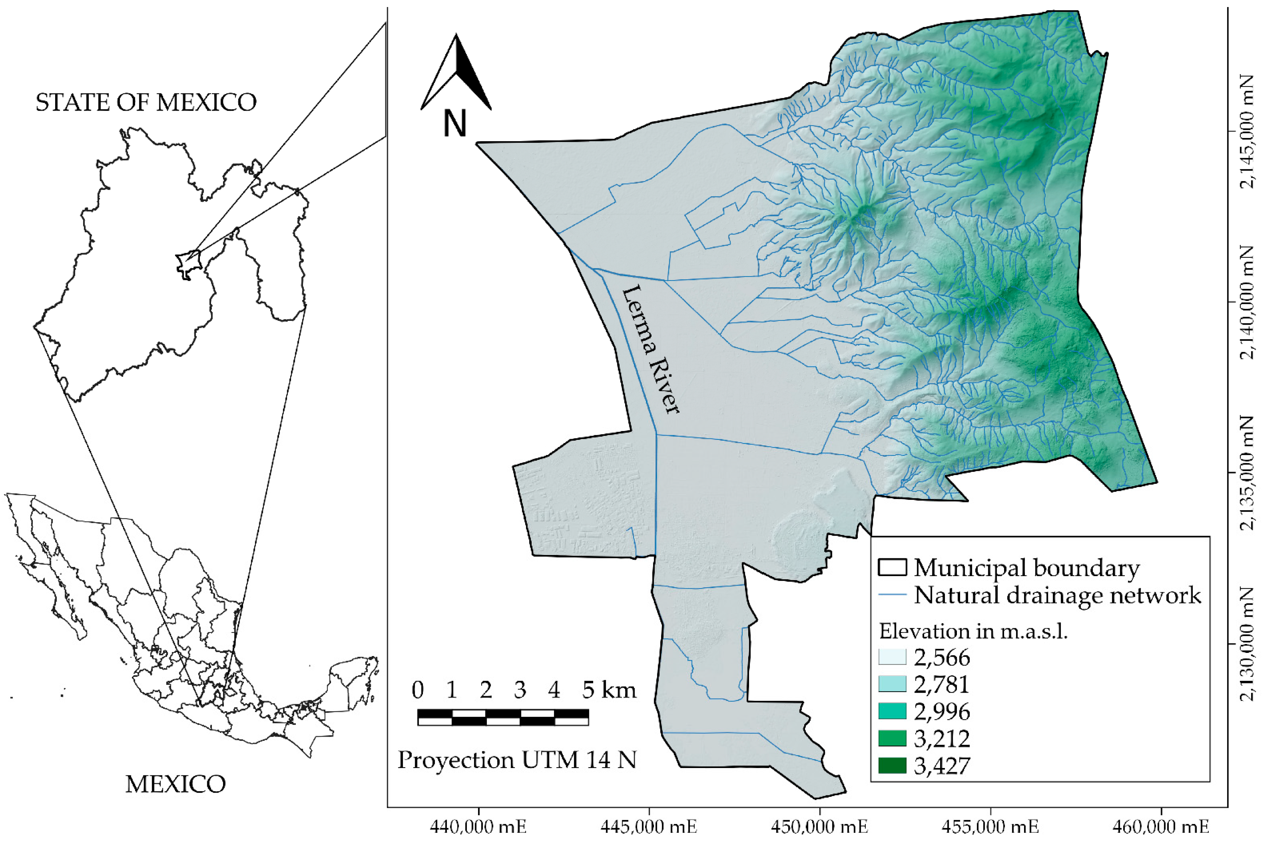
In central and southeastern Mexico, floods occur every year because of the intense rainfall during the period from June to October, with surface runoff caused by deforestation and also due to effects of climate change [25,26]. Although some previous studies have used SAR image analysis and processing methods to monitor recurrent floods in the southern part of the country, traditional classification techniques were used in most investigations. Some of them used Radarsat-2 and Sentinel-1 SAR images to track flooding using single and dual polarizations; others evaluated the Sentinel-1 data for describing the spatial and temporal variability of water bodies [27,28,29,30]. The objective of this research was to evaluate and compare the performance of two assembly algorithms: gradient boosting (GB) and random forest (RF) for different combinations of Sentinel-1 SAR images, Sentinel-2 optical images, indexes to detect water bodies, and DEMs for monitoring the extent and depth of flooding generated by excess rainfall.

2. Materials and Methods

2.1. Study Area

The study area is located in the Municipality of Lerma de Villada, State of Mexico, Mexico (Figure 1), and has a surface area of 230,810 km2 (23,081 ha) in an irregular polygon with a perimeter of 93,248 km. The study area has a minimum elevation of 2566.2 m above sea level (masl), and in the eastern part of the area, which comprises mountainous terrain, it reaches a maximum value of 3427 masl. The study area corresponds to the Lerma–Santiago hydrological region, whose natural drainage network captures runoff from the mountains in the east and transports it westward through tributaries of the Lerma River, whose path follows a course to the northwest of the State of Mexico (Figure 1).

2.2. Rainfall Data Analysis

The rainfall data for the year 2021 were analyzed, obtained from five stations near the study area (2RSMX, CGCMEX, COBMX, RECMX, and TROMX) of the National Meteorological Service [31]. To generate the spatial pattern of rainfall for the period 1 January to 30 September 2021, kriging interpolation was used based on statistical models that include autocorrelation. Only one year of rainfall data observation was analyzed (2021), as this was an atypical rainy year in the study area. In this analysis, the daily precipitation information covered two seasons: (a) the dry season (January to May), and the rainy season (June to September).

2.3. Satellite Images Used

Sentinel-1 and Sentinel-2 images were selected due to their spatial and temporal resolution; their timing in data acquisition also allows access the necessary images to cover the flood event in its entirety. Additionally, there are free access computational tools for preprocessing, as well as extensive experience in the use of this type of images in problems related to detection and classification [32].
Two Sentinel-1 SAR and two Sentinel-2 multispectral scenes were used, one from the dry season and one from the rainy season for each sensor (Table 1). The characteristics of the Sentinel-1 SAR images used were: C band, a spatial resolution of 10 m, acquisition form interferometric wide-swath (IW), processing level 1 (ground range detected or GRD), and dual polarization (VV and VH). For Sentinel-2, bands 4, 3, and 2 with 10 m original resolution, and bands 7, 6, and 5 with resampling, were used to obtain a spatial resolution of 10 m. The images were obtained from the Alaska Satellite Facility (ASF) platform (https://asf.alaska.edu/, accessed on 10 September 2021).

2.4. Software and Computing Requirements

Processing of SAR images was performed using the Sentinel-1 toolbox in the Sentinel application platform (SNAP) [33] and of Sentinel-2 images was performed with the semi-automatic classification plugin [34] extension of QGis Version 3.10.7.
The implementation of machine-learning algorithms was carried out in Python 3.7 language through the Scikit learn 0.21.3 [35] module in a Spyder 3.6 environment. Both vector and matrix mathematical operations were developed with Pandas 0.25.1, Numpy 1.16.5, and Matlab R2016a, with output graphs being constructed using Matplotlib 3.1.1 and Seaborn 0.9.0.

2.5. Sample Selection and Resampling

To incorporate pixel qualities and characteristics that correspond to each target class, the resampling process was performed on Sentinel-1 polarization VV and VH images and on the RGB false-color compounds (bands 4, 3, and 2) of Sentinel-2. The resampling was conducted with the binary classification approach, that is, there are two possible exclusive classes (1 if a pixel belongs to the “water” class, and 0 for the “non-water” class). Sample selection was developed in two phases:
(a)
In Phase 1, the coordinates (x, y) of a set of pixels representing the two target classes were obtained. This procedure was performed on a subset of the image of variable size to select pixels with greater detail. For this, three methods were used: (1) growth by region [36,37], (2) manual definition of the threshold, and (3) use of the entire subset. The method for manually defining the threshold and using the entire subset consisted of defining a threshold for binary segmentation based on analysis of the histogram of the subset and the graphic display. This procedure starts with the transformation of the input image to a single band. In the case of Sentinel-1 (SAR), only one polarization is used. Next, the histogram of the scene is calculated [7]. In the case of Sentinel-2, a limit value is defined that allows the separation of water bodies and that also allows a pixel-by-pixel validation on the RGB composite image. Before exporting the coordinates of the sampling pixels, the intra- and inter-class duplicates database was purged, based on the value of the RGB false-color pixels for the “non-water” class and backscatter (VV) values for the “water” class.
(b)
In Phase 2, the database of phase 1 was updated, and using the geographic coordinates, the pixel values were recovered for the following input combinations: RGB and HSV composite of Sentinel-2, Sentinel-1 VV, and VH polarization, and DEM and indices to detect bodies of water (Table 2). Bands 4, 3, and 2 of the Sentinel-2 image were assigned to generate the RGB composite. The HSV model represents color of three components: Hue (H), Saturation (S), and Value (V). In uniform spaces, the color difference (Euclidean distance) is proportional to the human perception of that difference. In this sense, RGB is not uniform [38]. The conversion from RGB to HSV was obtained from the OpenCV library, using the cvtColor function in Python-3.

2.6. Machine Learning Algorithms Used

Algorithms known as decision trees were introduced by Breiman et al., in 1984 [43]. These algorithms have a tree-like structure, starting with a root, followed by nodes that represent a division rule and give rise to branches on both sides. By successive divisions, one arrives at the sheets, which indicate the target classes. The decision tree is built recursively from top to bottom with the initial selection of the features to be used in each decision rule. The construction ends when all of the samples belong to the same class, the features to be subdivided are exhausted, and the maximum allowable depth of the structure has been reached [44]. The key hyperparameters that allow control of the creation of decision trees in the training process are (a) Max_features, (b) Min_samples_split, (c) Min_samples_leaf, and (d) Max_depth [45]. In this study, the GB and RF decision-tree-based ensemble algorithms were used, as described below.

2.6.1. Gradient Boosting

This assembly algorithm proposed by Friedman [46] trains decision trees sequentially. The process involves creating “Ne” (number of estimators), and for each tree, the algorithm is trained and corrected with the residual values of its predecessor. This approach allows a robust and powerful algorithm to be obtained after “Ne” iterations [47].
The cost function (L) that allows optimization of the division for each tree is the entropy expressed in Equation (1) [48]:
L = i = 1 N c y i log P i ( x )
where yi = 1 is the i-th response up to Nc (number of classes) ∈ {0, 1}, and Pi (x) = Pr(yi = 1|x), is the probability that input x generates an output and is equal to unity.

2.6.2. Random Forest

The RF assembly algorithm is based on decision trees and was proposed by Breiman in 2001 [49]. The process consists of training decision trees with different subsets of “Nce” (features with replacement) to create “Ne”.
The cost function (L) to be optimized indicates the impurity of the split in each tree, which is given by the Gini index [50] as
L = I G ( i ) = j = 1 N c p ( C j | i ) ( 1 p ( C j | i ) )  
where p(Cj|i) is the proportion of samples belonging to class j, and Nc represents the total number of classes for a particular node i.

2.7. The Training Algorithms

The approach used during training was cross validation. This involves optimizing the algorithms several times to obtain weighted ranking metrics. In this case, 10 cycles were performed, and in each one, 90% of the data was used to train the models, and the remaining 10% (which does not belong to the training set) was used to evaluate the model using validation metrics mentioned in Section 2.7.1.
Standard hyperparameters of each algorithm were selected, and data cross-validation was performed [51,52]. The process began with the definition of the number of partitions for cross-validation (Kf), whereby Kf subsets, disjoint and stratified with respect to the dependent variable, were generated for the dataset. The model was trained Kf times, and in each iteration, Kf-1 subsets were used for training, with the remainder being used for validation. In each iteration, the validation subset was changed, and at the end of the cycle, Kf trained models were obtained, allowing calculation of the indicators for comparison. The hyperparameters of the machine learning models found by the cross-validation processes were the following:
(a)
For Gradient Boosting (GB):
Loss function to be optimized (log_loss, binomial and multinomial deviation).
Learning rate (learning_rate = 0.1).
Number of estimators (n_estimators = 100).
Criterion to measure the quality of the branches (‘friedman_mse’, for the mean squared error with improvement score by Friedman).
Minimum samples for each internal node split (min_samples_split = 2).
Minimum number of samples to define a leaf (min_samples_leaf = 1).
Maximum depth (max_depth = 3).
Randomization seed (random_state = 1).
Maximum features (None, set equal to the number of features or attributes available).
(b)
For Random Forest (RF):
Number of trees that make up the forest (n_estimators = 100).
Function or criterion to measure the quality of the ramifications (gini index).
Maximum depth (None).
Minimum samples for each internal node split (min_samples_split = 2).
Minimum samples to define a leaf (min_samples_leaf = 1).
Maximum features or attributes (max_features = “sqrt”), square root of the number of features.
Randomization seed (random_state = 1).

2.7.1. Training Algorithms of Machine Learning Models for Flood Prediction

In the prediction stage, the classifier with the independent variables as inputs classified a pixel into two classes: “1, water” and “0, non-water”. Depending on the result of the classification and the actual (desired) label of the pixel, four possibilities arise: (a) true positive (VP), when a pixel is correctly classified as class 1; (b) false positive (FP), when a pixel of class “0” is wrongly classified as class 1 (type I error); (c) true negative (TN), when a pixel is correctly classified as class “0”; and (d) false negative (FN), when a pixel of class “1” is wrongly classified as class “0” (type II error).
To determine the global accuracy of the algorithms (PG), the relationship between the correctly classified values (VP + VN) and the total of the test set (VP + FP + VN + FN) was obtained. This parameter measures the performance of models on balanced samples, also considering the use of four auxiliary evaluation criteria or metrics (precision, sensitivity, F1 score, and Kappa), as described below.
Precision (P) is defined as the ability of the model to correctly classify class 1 pixels in a set whose labels are known and is calculated using Equation (3):
P = V P V P + F P
Sensitivity (S) measures the ability of the classifier to identify those pixels that represent the water class in a completely unrelated set. It is evaluated and calculated in decimal values using Equation (4):
S = V P V P + F N
The criteria of P and S follow inverse behavior curves and depend directly on the threshold that is defined to declare the model output as class 1. The harmonic mean of these criteria is better known as the F1 score and allows comparison of the evaluated models with greater certainty. In cases for which there are multiple target classes, it is convenient to use the mean of F1, known as F1 macro (F1m). F1 is calculated as
F 1 = 2 × P × S P + S
The Kappa index [53] is another discrete multivariable technique that can be used to evaluate the accuracy of algorithms. The KHAT (K) index is calculated using Equation (6) [54]:
K = N i = 1 r x i i i = 1 r ( x i + × x + i ) N 2 i = 1 r ( x i + × x + i )
where r is the total number of rows in the matrix; xii is the number of observations for the “ith” row and column; xi+ and x+i are the marginal totals for the i row and column, respectively; and N is the total number of observations.

2.8. Workflow

The workflow started with processing using optical Sentinel-2 [55,56] and SAR Sentinel-1 [57,58,59] data for the dry season to identify perennial water bodies (lagoons, rivers, and irrigation canals) through the growth model by region and manual definition of the threshold. The database was built with the independent variables, which were polarization (VH, VV, and VV/VH), RGB, HSV, and indexes (Table 2) to detect water bodies from Sentinel-2 bands. The clean database without duplicates between and inter-class allowed optimization of the models through cross-validation with Kf = 10 [60]. The classification accuracy of the standard models was evaluated and compared with the following indicators: P, S, F1, K, the ROC curve (ROC, receiver operating characteristic), and the area under the ROC curve (AUC, area under the curve). The best classifier generated the prediction for each pixel in the satellite images used in the dry and rainy seasons, with maps of flooded areas being calculated by area difference (Figure 2).

2.9. Input Combinations for Algorithm Training

Table 3 describes the inputs and combinations obtained from Sentinel-2 and Sentinel-1 for the dry and rainy seasons using the GB and RF algorithms. Three main inputs were generated: (a) Sentinel-2 (S2), (b) Sentinel-1 (S1), and (c) DEM.

2.10. Flood Extent

To determine the extent of flooding, the change in pixel classification between the two seasons was computed. Flooding was assigned for a change in pixel classification from 0 in the dry season to 1 in the rainy season, and permanent water was assigned for a value of 1 in both seasons.

2.11. Depth of Flooding

The DEM generated using LiDAR from sources E14A38 (2018) and E14A48 (2016) [61] was used to determine the depth of flooded areas by reclassifying the data every 0.50 m. Given the study area elevation range of 2567.5–3427.3 masl, the minimum elevation was used as the baseline for the reclassification and therefore for the depth of flooded areas. In addition, vector data were obtained from the hydrographic network (RH) sub-basin RH12Aa Almoloya-Otzolotepec region, Lerma-Santiago river basin [62], the pluvial drainage network, lagoons, and the great canal crossing the study area. The reclassification was carried out using the QGis reclass module. Other studies have been carried out using the DEM; for example, [19] used a Floodwater Depth Estimation Tool (FwDET), developed to augment remote sensing analysis by calculating water depth based solely on an inundation map with an associated digital elevation model (DEM). The results showed good correspondence, with an average difference of 0.18 m for the coastal (using a 1 m DEM) and 0.31 m for the riverine (using a 10 m DEM) case studies.

3. Results

3.1. Rainfall Record during 2021

The rainfall during September 2021 in the study area was the highest recorded monthly total in the year (201.22 mm) [31]. During the days of 4 to 7 September, excessive rainfall occurred in terms of both intensity and duration, which caused flooding and overflows of the Lerma River in the Lerma–Santiago basin. The minimum mean monthly precipitation from January to September of the five stations near the study area was 1.66 mm (January), and as the months passed, the cumulative precipitation increased to 815.85 mm by 30 September 2021 (Figure 3).

3.2. Samples Selected for Algorithm Training

For the Sentinel-2 RGB composite, a refined and unbalanced database of 62,400 samples (20,000 for the water class and 42,400 for the non-water class) was generated. Of these, 32,000 samples corresponded to the dry season (10,000 in the water class and 22,000 in the non-water class) (Figure 4A), and 30,400 samples for the rainy season (10,000 in the water class and 20,400 in the non-water class) (Figure 4B).

3.3. Evaluation of Algorithms to Determine Flooded Areas

Figure 5 shows the input images described in Table 3 used for training and evaluating the machine learning algorithms. HSV false-color composites of Sentinel-2 for the dry and rainy seasons are presented in Figure 5A and 5D, respectively, VV polarizations of Sentinel-1 for the dry and rainy seasons are presented in Figure 5B and 5E, respectively, and the DEM is shown in Figure 5C.

3.3.1. Results for Gradient Boosting Algorithm

For Sentinel-2 and the GB classification algorithm, for both the dry and rainy seasons, the best results were obtained with combination 8 (K = 0.9895 and 0.9716, respectively) (Table 4). For SAR Sentinel-1 and the GB algorithm, the best result for the dry season was obtained with combination 12 (K = 0.9574), and for the rainy season was obtained with combination 11 (K = 0.9560).
When combining Sentinel-2, Sentinel-1, and MDE using the GB algorithm, combination 15 gave the best result for the dry season (K = 0.9945) and combination 16 for the rainy season (K = 0.9905) (Table 4).

3.3.2. Results for Random Forest Algorithm

For Sentinel-2 and the RF classification algorithm, for both the dry and rainy seasons, the best results were obtained with combination 8 (K = 0.9885 and 0.9721, respectively) (Table 5). Similarly, with Sentinel-1 and the RF algorithm, for both the dry and rainy seasons, the best results were obtained with combination 11 (K = 0.9547 and 0.9554, respectively).
When combining Sentinel-2, Sentinel-1, and DEM using the RF algorithm, combination 15 gave the best result for the dry season (K = 0.9937) and combination 16 for the rainy season (K = 0.9878) (Table 5).

3.4. The Best Combinations for Determining Flooding According to Season and Algorithm

On the basis of the information in Table 4 and Table 5, the best input combinations for detecting permanent bodies of water in the dry and rainy seasons and flooded areas in the rainy season were able to be identified.

3.4.1. Dry Season

Both algorithms (RF and GB) showed good performance for combination 15 (Algorithm + Sentinel-2 HSV composite + Sentinel-1 VV polarization + MDE). However, a better classification was obtained with the GB algorithm; the performance indicators (F1m, AUC, and Kappa) are shown in Table 6, which were used to validate the results.
Values of indicators for evaluating the performance of the algorithms are presented in Table 7 and were obtained from the confusion matrix of the last test subset in the cross-validation phase (Kf = 10). The best-ranked algorithm was GB, with an overall accuracy of 99.81%. The performance error of the GB and RF algorithms is directly related to the false positive (FP) rate.
For the dry season, the GB algorithm predicted an extent of water bodies (surface area) of 968.43 ha (4.20% of the total study area), whereas the RF algorithm predicted an area of 836.6 ha (3.63% of the total study area) (Table 8).
The GB algorithm identified a greater extent of water bodies in the dry season compared with RF, although the distributions are similar for the two algorithms (Figure 6A,B). This is because both models use decision trees for classification.

3.4.2. Rainy Season

Both algorithms obtained the best results for the detection of floods in the rainy season with combination 16. The index that contributes best to flood detection is the AWEI index. A comparison of the performance of the two algorithms reveals that GB shows the best result than RF; the performance indicators (F1m, AUC, and Kappa) are shown in Table 9, which were used to validate the results.
Values of indicators for evaluating the performance of the algorithms are presented in Table 10 and were obtained from the confusion matrix of the last test subset in the cross-validation phase (Kf = 10). The GB algorithm showed the best performance when classifying the test set, with an overall accuracy (GP) of 99.67%, compared with 99.47% for RF. Compared with results for the dry season, the two analyzed models have lower classification accuracies because of type II errors, with a high rate of false negative classifications.
For the extent of permanent bodies of water and flooded areas in the rainy season, the GB algorithm identified 7.96% of the total area as being water, compared with 7.04% for RF (Table 11).
The GB algorithm correctly predicts flooded areas in agricultural areas located in valleys and transition zones (mountain slopes), as well as an increase in surface area along the left bank of the Lerma River and areas with urban infrastructure. The similarity of the pattern of flooded area for GB and RF can be seen in Figure 7A,B and is due largely to both of these algorithms being based on decision trees.

3.5. Extent of Flooding According to Season

Flooding was considered to be those pixels that were classified as “non-water“class during the dry season and as “water” class during the rainy season. With this criterion, the GB algorithm identified 1113.36 ha of flooding, and RF identified 670.46 ha of flooding (Table 12). The analysis of the extent of the flooding is based on the temporal change of the pixels as represented by the difference between Figure 6 (dry season) and Figure 7 (rainy season). The flooded areas are largely on the left bank of the Lerma River, agricultural plots in the Lerma valley, as well as intermittent stormwater channels in the catchment areas and runoff from the mountains into the Lerma valley (Figure 8). Regarding the evaluated algorithms, the difference between GB and RF lies in the compactness of the flooded regions identified by the evaluation metrics. Both algorithms have acceptable performance for flood identification and monitoring.

3.6. Depth of Flooded Areas

Agricultural plots of the center and north of the valley show flooded areas with depths of <0.5 m. In other areas, such as Lagoon, depths ranging from 1.0 to 1.5 m were observed. The left bank area of Lerma river, which is located in the west of the study area, showed depths of >2 m from overflow. In hillside areas, small valleys retain runoff water and flood water (Figure 9) generated by the intense rainfalls that occurred from 4 to 7 September 2021.

4. Discussion

The presence of clouds, fog, and atmospheric particles in Sentinel-2 optical images can place limitations on detecting phenomena during rainy periods, as such conditions decrease solar illumination. During image processing, it is necessary to homogenize the histograms and normalize values of the RGB composite [63]. In SAR image processing, backscatter values are converted to backscatter coefficients (dB) to increase scene contrast and enhance visual differences between target classes.
The results obtained using machine learning algorithms (models) in this research indicate that, of the analyzed inputs, the combination of Sentinel-2, Sentinel-1, and DEM obtained more reliable results than other combinations [64,65], and the more robust and efficient model was gradient boosting algorithm to classify water bodies and flooded areas. The use of optical images with SAR images forms a complementation that can reduce Type I and II classification errors in the two analyzed machine learning algorithms (GB and RF). However, if a multiclass classification is to be carried out, then the use of optical images is necessary, as it allows a wide variety of shades and textures to be distinguished, which can be perfectly correlated to detect different uses and land covers, such as bodies of water and flooded areas [66,67]. In addition, SAR images can be used to identify bodies of water with aquatic vegetation, lagoons, rivers, lakes, and irrigation canals using VV polarization; however, the potential of SAR for monitoring floods is limited by the similarity of backscatter values in (shallow) flooded areas with soils without vegetation with high moisture content [68].
For the dry season, the utilized algorithms (GB and RF) detect similar regions of water bodies. The difference between the output maps lies in the compact regions, where the GB algorithm detects a larger area of water bodies than RF. For this season, the GB algorithm has the best performance for combination 15, generated by using Sentinel 2, Sentinel-1, and DEM (HSV composite, VV polarization, and DEM) with F1m = 0.997, AUC = 0.999, and K = 0.994.
For the rainy season, the models detect very similar spatial distributions of water bodies and flooded areas. There is a difference in the number of pixels that make up each region: GB identifies 1835.7 ha of flooded areas, and RF identifies 1623.98 ha. This difference is due to the identification by GB of pixels as “water” in small valleys located on the slopes of mountains. The best combination for both the RF and GB algorithms for the rainy season is combination 8, with F1m = 0.9861 and K = 0.9721 and F1m = 0.9858 and K = 0.9716, respectively.
In the comparison of the indexes derived from Sentinel-2 for detecting bodies of water for both algorithms (GB and RF); the best performance for the dry season is obtained with the reformulated automated water extraction index (AWEISH, combination 7) [42]; and the best performance for the rainy season is obtained with the automated water withdrawal index (AWEI, combination 6) [42]. The performance of the models does not improve significantly, when these indexes are integrated but the classification accuracy of the models increases with integration with the DEM.
According to Table 6 and 
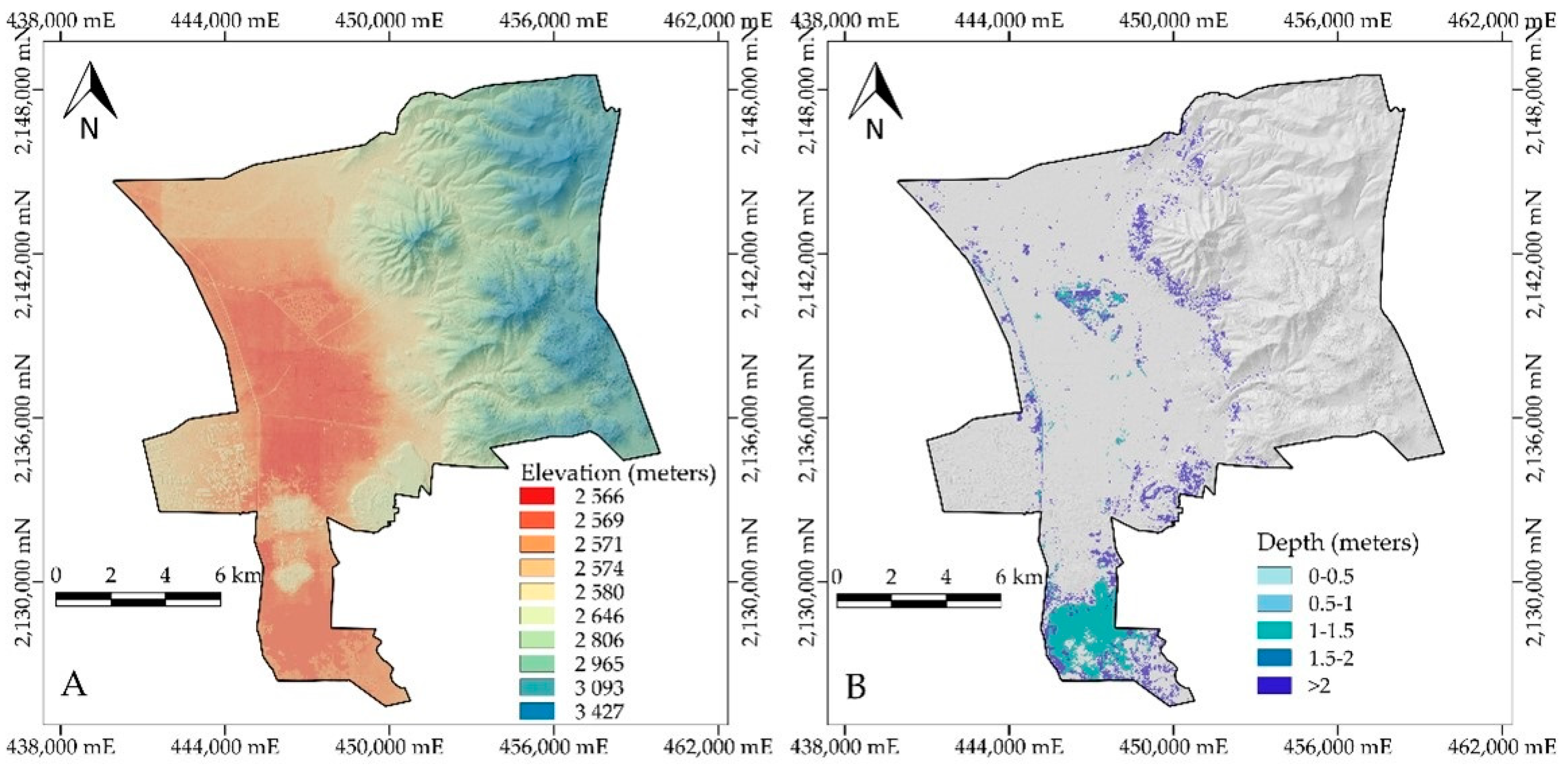
Table 9, the GB algorithm reports an extent of flooded areas of 1113.36 ha, and the evaluation metrics show that this model is superior to RF. The maps of flood extent obtained with both algorithms show a high degree of similarity. The depth of flooding in agricultural plots located in the central part of the Lerma valley and on the left bank of the Lerma River is less than 1 m, but in some parts of the lagoons, depths of 1–2 m are observed.
One of the advantages of this research is that the proposed methodology generates maps that show the extent of floods in a short time, whose results are validated using comparison metrics (F1m, AUC, and Kappa) using the best model.

5. Conclusions

In this study, we assessed 16 combinations of Sentinel-1 synthetic aperture radar (SAR) images, Sentinel-2 optical images, and DEM data to evaluate the performance of two widely used machine learning algorithms for providing information about flooding extent and depth, with a case study of flooding in the Municipality of Lerma de Villada, central Mexico.
To identify flooded areas, the combination of Sentinel-2 optical images, SAR Sentinel-1, and DEM, with GB and RF algorithms, gives more reliable results if we used only Sentinel-2 or Sentinel-1 for binary classification (water and non-water).
Determination of flooded areas requires independently analyzing the two seasons (dry and rainy) because meteorological conditions strongly affect the optical images in the rainy season and consequently generate a combined model that predicts high numbers of false positives.
For the three analysis inputs (Sentinel-2 + MDE, Sentinel-1 + MDE, and Sentinel-2 + Sentinel-1 + DEM) for both seasons (dry and rainy), the ensemble algorithms (GB and RF) show acceptable performance, with GB being slightly superior according to performance metrics.
For the detection of bodies of water in the dry season, the metrics indicate that the best algorithm is GB with combination 15 (F1m = 0.9973, AUC = 0.9999, K = 0.9945); however, the model gives a 0.27% classification error on the set of samples with which it was trained and evaluated. For the identification of flooded areas in the rainy season, with the same GB algorithm, the best results are obtained with combination 16 (F1m = 0.9953, AUC = 0.9999, and K = 0.9905); however, the model shows a 0.47% classification error on the set of samples with which it was trained and evaluated.
The GB algorithm generates the best result for the extent of flooding, with an area of 1113.36 hectares, with flooding depth ranging is <1.0 m.
The output maps of both the extent and depth of flooding should allow planning and execution of flood mitigation actions in a more timely manner and with a higher degree of accuracy than could otherwise be achieved.
This research aims to be the basis and approach to the implementation of machine learning algorithms applied to flood monitoring in southeastern Mexico. For future work, it is recommended to incorporate field validations and case studies elsewhere in order to obtain better calibrated models.

Author Contributions

Conceptualization, J.S.-R. and Y.M.F.-O.; methodology, J.S.-R. and J.P.A.-A.; software, J.P.A.-A.; validation, J.S.-R., Y.M.F.-O., J.P.A.-A. and E.D.S.-R.; formal analysis, J.P.A.-A.; investigation, J.S.-R. and G.M.-G.; resources, M.J.E.-M.; data curation, M.E.R.-G.; writing—original draft preparation, J.P.A.-A. and J.S.-R.; writing—review and editing, J.S.-R.; visualization, M.E.R.-G. and Y.M.F.-O.; supervision, J.S.-R.; project administration, Y.M.F.-O.; funding acquisition, Y.M.F.-O. All authors have read and agreed to the published version of the manuscript.

Funding

This work was supported by Colegio de Postgraduados (Mexico), funding number: 4306. The contents of this paper are solely the responsibility of the authors and do not necessarily represent the official views of the sponsors.

Institutional Review Board Statement

Not applicable.

Informed Consent Statement

Not applicable.

Data Availability Statement

The data that support the findings of this study are in this paper.

Conflicts of Interest

The authors declare no conflict of interest.

References

  1. IPCC. Summary for Policymakers. In Climate Change 2021: The Physical Science Basis, Contribution of Working Group to the Sixth Assessment Report of the Intergovernmental Panel on Climate Change; Masson-Delmotte, V., Zhai, P., Pirani, A., Connors, S.L., Péan, C., Berger, S., Caud, N., Chen, Y., Goldfarb, L., Gomis, M.I., et al., Eds.; IPCC: Geneva, Switzerland; Cambridge University: Cambridge, UK, 2021; pp. 1–40. [Google Scholar]
  2. NSTC. Science and Technology to Support Fresh Water Availability in the United States; National Science and Technology Council: Washington, DC, USA, 2004; pp. 1–19.
  3. Futrell, J.H.; Gephart, R.E.; Kabat, E.; McKnight, D.M.; Pyrtle, A.; Schimel, J.P.; Smyth, R.L.; Skole, D.L.; Wilson, J.L. Water: Challenges at the intersection of human and natural systems. NSF/DOE Tech. Rep. 2005, PNWD-3597, 1–50. [Google Scholar] [CrossRef] [Green Version]
  4. NRC. When Weather Matters: Science and Service to Meet Critical Societal Needs; National Academies Press: Washington, DC, USA, 2010; pp. 1–198. [Google Scholar]
  5. Hao, C.; Yunus, A.P.; Silva-Subramanian, S.; Avtar, R. Basin-wide flood depth and exposure mapping from SAR images and machine learning models. J. Environ. Manag. 2021, 297, 113367. [Google Scholar] [CrossRef] [PubMed]
  6. Soria-Ruíz, J.; Fernández-Ordoñez, Y.M.; Chapman, B. Radarsat-2 and Sentinel-1 SAR to detect and monitoring flooding areas in Tabasco, México. In Proceedings of the 2021 IEEE International Geoscience and Remote Sensing Symposium IGARSS, Brussels, Belgium, 11–16 July 2021; pp. 1323–1326. [Google Scholar]
  7. Carreño-Conde, F.; De Mata-Muñoz, M. Flood monitoring based on the study of Sentinel-1 SAR images: The Ebro river case study. Water 2019, 11, 2454. [Google Scholar] [CrossRef] [Green Version]
  8. Schlaer, S.; Matgen, P.; Hollaus, M.; Wagner, W. Flood detection from multi-temporal SAR data using harmonic analysis and change detection. Int. J. Appl. Earth Obs. Geoinf. 2015, 38, 15–24. [Google Scholar] [CrossRef]
  9. Pulvirenti, L.; Chini, M.; Pierdicca, N.; Guerriero, L.; Ferrazzoli, P. Flood monitoring using multi-temporal COSMO-SkyMed data: Image segmentation and signature interpretation. Remote Sens. Environ. 2011, 115, 990–1002. [Google Scholar] [CrossRef]
  10. Refice, A.; Zingaro, M.; D’Addabbo, A.; Chini, M. Integrating C- and L-band SAR imagery for detailed flood monitoring of remote vegetated areas. Water 2020, 12, 2745. [Google Scholar] [CrossRef]
  11. Konapala, G.; Kumar, S.V.; Khalique-Ahmad, S. Exploring Sentinel-1 and Sentinel-2 diversity for flood inundation mapping using deep learning. ISPRS J. Photogramm. Remote Sens. 2021, 180, 163–173. [Google Scholar] [CrossRef]
  12. Rahman, M.R.; Thakur, P.K. Detecting, mapping and analysing of flood water propagation using synthetic aperture radar (SAR) satellite data and GIS: A case study from the Kendrapara District of Orissa State of India. Egypt. J. Remote Sens. Space Sci. 2017, 21, S37–S41. [Google Scholar] [CrossRef]
  13. Xu, Y.; Xiao-Chun, Z.; Xiu-Gui, W.; Yu, Z. Flood disaster monitoring based on Sentinel-1 data: A case study of Sihu Basin and Huaibei Plain, China. Water Sci. Eng. 2021, 14, 87–96. [Google Scholar] [CrossRef]
  14. Cai, Y.; Li, X.; Zhang, M.; Lin, H. Mapping wetland using the object-based stacked generalization method based on multi-temporal optical and SAR data. Int. J. Appl. Earth Obs. Geoinf. 2020, 92, 102164. [Google Scholar] [CrossRef]
  15. Atirah, N.; Fikri, A.; Khairunniza, S.; Razif, M.; Mijic, A. The use of LiDAR-Derived DEM in flood applications: A review. Remote Sens. 2020, 12, 2308. [Google Scholar] [CrossRef]
  16. Munawar, H.S.; Hammad, A.W.A.; Waller, S.T. Remote sensing methods for flood prediction: A review. Sensors 2022, 22, 960. [Google Scholar] [CrossRef] [PubMed]
  17. Polat, N.; Uysal, M.; Toprak, A.S. An investigation of DEM generation process based on LiDAR data filtering, decimation, and interpolation methods for an urban area. Measurement 2015, 75, 50–56. [Google Scholar] [CrossRef]
  18. Avand, M.; Kuriqi, A.; Khazaei, M.; Ghorbanzadeh, O. DEM resolution effects on machine learning performance for flood probability mapping. J. Hydro-Environ. Res. 2022, 40, 1–16. [Google Scholar] [CrossRef]
  19. Cohen, S.; Raney, A.; Munasinghe, D.; Derek-Loftis, J.; Molthan, A.; Bell, J.; Rogers, L.; Galantowicz, J.; Robert-Brakenridge, G.; Kettner, A.J.; et al. The Floodwater Depth Estimation Tool (FwDET v2.0) for improved remote sensing analysis of coastal flooding. Nat. Hazards Earth Syst. Sci. 2019, 19, 2053–2065. [Google Scholar] [CrossRef] [Green Version]
  20. Xie, Q.; Wang, J.; Lopez-Sanchez, J.M.; Peng, X.; Liao, C.; Shang, J.; Zhu, J.; Fu, H.; Ballester-Berman, J.D. Crop height estimation of corn from multi-year Radarsat-2 polarimetric observables using machine learning. Remote Sens. 2021, 13, 392. [Google Scholar] [CrossRef]
  21. Liang, J.; Liu, D. A local thresholding approach to flood water delineation using Sentinel-1 SAR imagery. ISPRS J. Photogramm. Remote Sens. 2019, 159, 53–62. [Google Scholar] [CrossRef]
  22. Shahabi, H.; Shirzadi, A.; Ghaderi, K.; Omidvar, E.; Al-Ansari, N.; Clague, J.; Geertsema, M.; Khosravi, K.; Amini, A.; Bahrami, S. Flood detection and susceptibility mapping using Sentinel-1 remote sensing data and a Machine Learning approach: Hybrid intelligence of bagging ensemble based on K-Nearest Neighbor classifier. Remote Sens. 2020, 12, 266. [Google Scholar] [CrossRef] [Green Version]
  23. Hasanuzzaman, M.; Islam, A.; Bera, B.; Kumar Shit, P. A comparison of performance measures of three machine learning algorithms for flood susceptibility mapping of river Silabati (tropical river, India). Phys. Chem. Earth 2022, 127, 103198. [Google Scholar] [CrossRef]
  24. Chen, W.; Li, Y.; Xue, W.; Shahabi, H.; Li, S.; Hong, H.; Wang, X.; Bian, H.; Zhang, S.; Pradhan, B. Modeling flood susceptibility using data-driven approaches of Naïve Bayes Tree, alternating Decision Tree, and Random Forest methods. Sci. Total Environ. 2020, 701, 134979. [Google Scholar] [CrossRef]
  25. Arreguín-Cortés, F.G.; Rubio-Gutiérrez, H. Análisis de las inundaciones en la planicie tabasqueña en el periodo 1995–2010. Tecnol. Cienc. Agua 2014, 5, 3. [Google Scholar]
  26. Perevochtchikova, M.; Lezama de la Torre, J.L. Causas de un desastre: Inundaciones del 2007 en Tabasco, México. J. Lat. Am. Geogr. 2010, 9, 73–98. [Google Scholar] [CrossRef]
  27. Fernández-Ordoñez, Y.M.; Soria-Ruiz, J.; Leblon, B.; Macedo-Cruz, A.; Ramírez-Guzmán, M.E.; Escalona-Maurice, M. Imágenes de radar para estudios territoriales, caso: Inundaciones en Tabasco con el uso de imágenes SAR Sentinel-1A y Radarsat-2. Rev. Int. Estad. Geogr. 2020, 11, 4–21. [Google Scholar]
  28. López-Caloca, A.A.; Tapia-Silva, F.O.; López, F.; Pilar, H.; Ramírez-González, A.O.; Rivera, G. Analyzing short term spatial and temporal dynamics of water presence at a basin-scale in Mexico using SAR data. GISci. Remote Sens. 2020, 57, 985–1004. [Google Scholar] [CrossRef]
  29. López-Caloca, A.A.; Valdiviezo-Navarro, J.C.; Tapia-Silva, F.O. Tracking short-term seasonally flooded areas to understand the dynamics of the Coatzacoalcos river in Veracruz, Mexico. J. Appl. Remote Sens. 2021, 15, 4. [Google Scholar] [CrossRef]
  30. Amani, M.; Brisco, B.; Mahdavi, S.; Ghorbanian, A.; Moghimi, A.; DeLancey, E.R.; Merchant, M.; Jahncke, R.; Fedorchuk, L.; Mui, A.; et al. Evaluation of the Landsat-Based Canadian wetland inventory map using multiple sources: Challenges of large-scale wetland classification using remote sensing. IEEE J. Sel. Top. Appl. Earth Obs. Remote Sens. 2021, 14, 32–52. [Google Scholar] [CrossRef]
  31. Servicio Meteorológico Nacional (SMN). Resúmenes Mensuales de Temperaturas y Lluvia. Available online: https://smn.conagua.gob.mx/es/climatologia/temperaturas-y-lluvias/resumenes-mensuales-de-temperaturas-y-lluvias (accessed on 5 October 2021).
  32. European Spatial Agency (ESA); Scientific Exploitation of Operational Missions (SEOM). Sentinel Application Platform (SNAP 7.0). 2021. Available online: http://step.esa.int/main/download/snap-download/ (accessed on 5 August 2021).
  33. Tarpanelli, A.; Mondini, A.; Camici, S. Effectiveness of Sentinel-1 and Sentinel-2 for flood detection assessment in Europe. Nat. Hazards Earth Syst. Sci. 2022, 22, 2473–2489. [Google Scholar] [CrossRef]
  34. Congedo, L. Semi-Automatic Classification Plugin: A Python tool for the download and processing of remote sensing images in QGIS. J. Open Source Softw. 2021, 6, 3172. [Google Scholar] [CrossRef]
  35. Pedregosa, F.; Varoquaux, G.; Gramfort, A.; Michel, V.; Thirion, B.; Grisel, O.; Blondel, M.; Prettenhofer, P.; Weiss, R.; Dubourg, V.; et al. Scikit-learn: Machine learning in Python. J. Mach. Learn. Res. 2011, 12, 2825–2830. [Google Scholar]
  36. Mehnert, A.; Jackway, P. An improved seeded region growing algorithm. Pattern Recognit. Lett. 1997, 18, 1065–1071. [Google Scholar] [CrossRef]
  37. Li, W.; Du, Y.; Li, H.; Wang, X.; Zhu, J. Decision tree algorithm based on regional growth. Proc. Sci. 2015, 6, 1–7. [Google Scholar]
  38. Chernov, V.; Alander, J.; Bochko, V. Integer-based accurate conversion between RGB and HSV color spaces. Comput. Electr. Eng. 2015, 46, 328–337. [Google Scholar] [CrossRef]
  39. Xu, H. Modification of normalised difference water index (NDWI) to enhance open water features in remotely sensed imagery. Int. J. Remote Sens. 2006, 14, 3025–3033. [Google Scholar] [CrossRef]
  40. Rogers, A.S.; Kearney, M.S. Reducing signature variability in unmixing coastal marsh thematic mapper scenes using spectral indices. Int. J. Remote Sens. 2004, 25, 2317–2335. [Google Scholar] [CrossRef]
  41. McFeeters, S.K. The use of the normalized difference water index (NDWI) in the delineation of open water features. Int. J. Remote Sens. 1996, 17, 1425–1432. [Google Scholar] [CrossRef]
  42. Feyisa, G.L.; Meilby, H.; Fensholt, R.; Proud, S.R. Automated water extraction index: A new technique for surface water mapping using Landsat imagery. Remote Sens. Environ. 2014, 140, 23–35. [Google Scholar] [CrossRef]
  43. Breiman, L.; Friedman, J.H.; Olshen, R.A.; Stone, C.J. Classification and Regression Trees; Routledge: Oxfordshire, UK, 1984; 368p. [Google Scholar] [CrossRef]
  44. Geurts, P.; Ernst, D.; Wehenkel, L. Extremely randomized trees. Mach. Learn. 2006, 63, 3–42. [Google Scholar] [CrossRef] [Green Version]
  45. Swamynathan, M. Mastering Machine Learning with Python in Six Steps; Apress: New York, NY, USA, 2017; pp. 1–374. [Google Scholar] [CrossRef]
  46. Friedman, J. Greedy function approximation: A gradient boosting machine. Ann. Stat. 2001, 29, 1189–1232. [Google Scholar] [CrossRef]
  47. Si, M.; Du, K. Development of a predictive emissions model using a gradient boosting machine learning method. Environ. Technol. Innov. 2020, 20, 101028. [Google Scholar] [CrossRef]
  48. Tangirala, S. Evaluating the impact of GINI index and information gain on classification using decision tree classifier algorithm. Int. J. Adv. Comput. Sci. Appl. 2020, 11, 612–619. [Google Scholar] [CrossRef] [Green Version]
  49. Breiman, L. Random forests. Mach. Learn. 2001, 45, 5–32. [Google Scholar] [CrossRef] [Green Version]
  50. Gini, C. Variability and Mutability. In Memorie Di Metodologica Statistica; Pizetti, E., Salvemini, T., Eds.; Libreria Eredi Virgilio Veschi: Rome, Italy, 1912. [Google Scholar]
  51. Raschka, S. Model Evaluation, Model Selection, and Algorithm Selection in Machine Learning; Department of Statistics, University of Wisconsin–Madison: Madison, WI, USA, 2018; pp. 1–49. [Google Scholar]
  52. Raschka, S.; Mirjalili, V. Python Machine Learning, 2nd ed.; Packt Publishing Ltd.: Birmingham, UK, 2017; pp. 1–850. [Google Scholar]
  53. Cohen, J. A coefficient of agreement for nominal scales. Educ. Psychol. Meas. 1960, 20, 37–46. [Google Scholar] [CrossRef]
  54. Congalton, R.G. A Review of assessing the accuracy of classifications of remotely rensed data. Remote Sens. Environ. 1991, 37, 35–46. [Google Scholar] [CrossRef]
  55. Clerici, N.; Valbuena-Calderón, C.A.; Posada, J.M. Fusion of Sentinel-1A and Sentinel-2A data for land cover mapping: A case study in the lower Magdalena region, Colombia. J. Maps 2017, 13, 718–726. [Google Scholar] [CrossRef] [Green Version]
  56. Gašparovic, M.; Klobucar, D. Mapping floods in lowland forest using Sentinel-1 and Sentinel-2 data and an object-based approach. Forests 2021, 12, 553. [Google Scholar] [CrossRef]
  57. Congedo, L. Tutorial 2. Available online: https://semiautomaticclassificationmanual-v5.readthedocs.io/es/latest/tutorial_2.html (accessed on 5 October 2021).
  58. Baillarin, S.J.; Meygret, A.; Dechoz, C.; Petrucci, B.; Lacherade, S.; Tremas, T.; Isola, C.; Martimort, P.; Spoto, F. Sentinel-2 level 1 products and image processing performances. In Proceedings of the 2012 IEEE International Geoscience and Remote Sensing Symposium, Munich, Germany, 22–27 July 2012; pp. 197–202. [Google Scholar]
  59. Congedo, L. Breve Introducción a la Teledetección. Available online: https://semiautomaticclassificationmanual-v5.readthedocs.io/es/latest/remote_sensing.html#image-conversion-to-reflectance (accessed on 5 October 2021).
  60. MathWorks. Cvpartition. Available online: https://la.mathworks.com/help/stats/cvpartition.html (accessed on 5 October 2021).
  61. Instituto Nacional de Estadística y Geografía (INEGI). Mapas. Available online: https://www.inegi.org.mx/app/mapas/?tg=1015 (accessed on 5 September 2021).
  62. Comisión Nacional Para el Conocimiento y Uso de la Biodiversidad (CONABIO). Portal de Geoinformación. 2021. Available online: http://www.conabio.gob.mx/informacion/gis/ (accessed on 5 September 2021).
  63. Yang, Y.; Liu, Y.; Zhou, M.; Zhang, S.; Zhan, W.; Sun, C.; Duan, Y. Landsat 8 OLI image based terrestrial water extraction from heterogeneous backgrounds using a reflectance homogenization approach. Remote Sens. Environ. 2015, 171, 14–32. [Google Scholar] [CrossRef]
  64. Huang, M.; Jin, S. Rapid flood mapping and evaluation with a supervised classifier and change detection in Shouguang using Sentinel-1 SAR and Sentinel-2 optical data. Remote Sens. 2020, 12, 2073. [Google Scholar] [CrossRef]
  65. Bioresita, F.; Puissant, A.; Stumpf, A.; Malet, J.P. Fusion of Sentinel-1 and Sentinel-2 image time series for permanent and temporary surface water mapping. Int. J. Remote Sens. 2019, 40, 9026–9049. [Google Scholar] [CrossRef]
  66. Solórzano, J.; Mas, J.; Gao, Y.; Gallardo, A. Land use land cover classification with U-Net: Advantages of combining Sentinel-1 and Sentinel-2 imagery. Remote Sens. 2021, 13, 3600. [Google Scholar] [CrossRef]
  67. Gašparović, M.; Jogun, T. The effect of fusing Sentinel-2 bands on land-cover classification. Int. J. Remote Sens. 2018, 39, 822–841. [Google Scholar] [CrossRef]
  68. Chini, M.; Pelich, R.; Pulvirenti, L.; Pierdicca, N.; Hostache, R.; Matgen, P. Sentinel-1 InSAR coherence to detect floodwater in urban areas: Houston and hurricane harvey as a test case. Remote Sens. 2019, 11, 107. [Google Scholar] [CrossRef]
Figure 1. Study area in the Municipality of Lerma de Villada, State of Mexico.
Atmosphere 13 01852 g001
Figure 2. Workflow for preprocessing, sample selection, training, evaluation of machine learning algorithms, and generation of thematic maps.
Atmosphere 13 01852 g002
Figure 3. Mean and cumulative rainfall from January to September 2021.
Atmosphere 13 01852 g003
Figure 4. Distribution of samples selected for algorithm training for the dry (A) and rainy (B) seasons.
Atmosphere 13 01852 g004
Figure 5. Input images for the evaluation of machine learning algorithms: Sentinel-2 (A,D) and Sentinel-1 (B,E) for the dry and rainy seasons, respectively, and the DEM (C).
Atmosphere 13 01852 g005
Figure 6. Extent of water bodies obtained using the GB (A) and RF (B) algorithms with the best combination (combination 15) for the dry season.
Atmosphere 13 01852 g006
Figure 7. Extent of flooding in the rainy season with gradient boosting (A) and random forest (B) algorithms.
Atmosphere 13 01852 g007
Figure 8. Extent of water bodies in the dry season and flooded areas in the rainy season calculated from the spatial and temporal analysis of pixels with gradient boosting (A) and random forest (B) algorithms.
Atmosphere 13 01852 g008
Figure 9. (A) Elevation distribution over the study area (DEM from LiDAR) and (B) depth of flooded areas.
Atmosphere 13 01852 g009
Table 1. Characteristics of the Sentinel-1 and Sentinel-2 satellite images used.
SatelliteDateSeasonResolution (m)ProcessingPolarization
and Bands
Orbit and
Clouds (%)
Sentinel-110 April 2021Dry10IW 1 GRHVH, VVDescending
Sentinel-211 April 2021Dry10MSIL1C4, 3, 2, 7, 6, 55.8
Sentinel-17 September 2021Rainy10IW 1 GRHVH, VVDescending
Sentinel-28 September 2021Rainy10MSIL1C4, 3, 2, 7, 6, 528.8
Table 2. Indexes used to detect water bodies in multispectral images.
IndexReference
M N D W I 1 = G S W I R 1 G + S W I R 1 [39]
M N D W I 2 = R S W I R 1 R + S W I R 1 [40]
N D W I = G N I R G + N I R [41]
A W E I = 4 × ( G S W I R 1 ) ( 0.25 × N I R + 2.75 × S W I R 2 ) [42]
A W E I S H = B + 2.5 × G 1.5 × ( N I R + S W I R 1 ) 0.25 × S W I R 2 [42]
Where: MNDWI1 is the modification of normalized difference water index; MNDWI2 is the water difference index normalized modified by Rogers and Kearney; NDWI is the normalized difference index of water; AWEI is the automated water extraction index; AWEISH is the automated water extraction index.
Table 3. Description of the inputs and their combinations for training and evaluating machine learning algorithms.
EntryCombinationDescription
S21Algorithm + RGB composite of S2.
S22Algorithm + HSB composite of S2
S23Algorithm + HSV composite of S2 + MNDWI1 index.
S24Algorithm + HSV composite of S2 + MNDWI2 index.
S25Algorithm + HSV composite of S2 + NDWI index.
S26Algorithm + HSV composite of S2 + AWEI index.
S27Algorithm + HSV composite of S2 + AWEISH index.
S2, DEM8Algorithm + HSV composite of S2 + DEM
S2, DEM9Algorithm + H, V bands from HSV composite of S2 + DEM
S110Algorithm + (VH, VV) dual polarization of S1.
S1, DEM11Algorithm + (VH, VV) dual polarization of S1 + DEM
S1, DEM12Algorithm + (VH, VV) dual polarization of S1 + (VV/VH) polarization of S1 + DEM
S2, S113Algorithm + HSV composite of S2 + VH polarization of S1.
S2, S114Algorithm + HSV composite of S2 + VV polarization of S1.
S2, S1, DEM15Algorithm + HSV composite of S2 + VV polarization of S1 + DEM
S2, S1, DEM16Algorithm + H, V bands from HSV composite of S2 + VV polarization of S1 + AWEI index + DEM
Table 4. Values of performance indicators obtained using the GB algorithm for all combinations for the dry and rainy seasons.
CombinationF1mAUCKappaF1mAUCKappa
DryRainy
10.98150.99810.96310.89580.95950.7916
20.98160.99830.96320.89350.9610.7871
30.98430.99860.96860.89350.9610.7871
40.98350.99850.9670.89350.9610.7871
50.98390.99850.96770.89350.9610.7871
60.98380.99860.96760.92090.97530.8419
70.98450.99860.96890.91710.97360.8343
80.99480.99980.98950.98580.99880.9716
90.99270.99970.98540.9830.99840.9659
100.95380.99120.90760.94880.99030.8975
110.97860.99840.95710.9780.99850.956
120.97870.99840.95740.97760.99840.9552
130.99160.99940.98320.97480.99680.9497
140.99450.99960.9890.97540.99730.9508
150.99730.99990.99450.99440.99980.9887
160.99680.99990.99360.99530.99990.9905
Notes: F1m is the F1 score for the two target classes; AUC is the area under the ROC curve; Kappa is the K coefficient.
Table 5. Performance indicators obtained using the RF algorithm for all combinations in the dry and rainy seasons.
Combination F 1 m AUCKappa F 1 m AUCKappa
Dry SeasonRainy Season
10.98120.99610.96230.88660.94940.7732
20.98050.99560.9610.88590.94990.7718
30.9840.99760.96810.8850.94960.7701
40.98370.99680.96750.8850.94960.7701
50.98340.99720.96680.8850.94960.7777
60.98320.99740.96640.920.97360.8444
70.98480.99710.96950.91670.97060.8334
80.99420.99950.98850.98610.9980.9721
90.99210.9990.98430.98250.99710.9649
100.94840.98460.89680.94330.98330.8866
110.97740.99730.95470.97770.99770.9554
120.97710.99740.95430.97720.99740.9543
130.9920.99830.98390.97410.99520.9482
140.99440.99880.98870.9750.99520.9555
150.99690.99960.99370.99330.99960.9866
160.99630.99970.99260.99390.99960.9878
Notes: F1m is the F1 score for the two target classes; AUC is the area under the ROC curve; Kappa is the K coefficient.
Table 6. Comparison metrics obtained for the GB and RF algorithms for the best combination in the dry season.
AlgorithmCombination F 1 m AUCKappa
GB150.99730.99990.9945
RF150.99690.99960.9937
Note: F 1 m is the mean F1 score for the two target classes (water and non-water).
Table 7. Indicators of the performance of algorithms obtained from the confusion matrix for the dry season.
AlgorithmCombinationVPFPVNFNPG (%)
GB159955219910.998
RF159928219820.996
Notes: VP is true positive values, FP is false positive values, VN is true negative values, FN is false negative values, and PG is global precision.
Table 8. Extent of water bodies identified by the two algorithms for the dry season.
AlgorithmCombinationExtent of
Water Bodies
(ha)(%)
GB15968.434.20
RF15836.63.63
Table 9. Comparison metrics obtained from GB and RF algorithms for the best combination for the rainy season.
AlgorithmCombination F 1 m AUCKappa
GB160.99530.99990.9905
RF160.99390.99960.9878
Note: F 1 m is the mean F1 score for the two target classes (water and non-water).
Table 10. Indicators of the performance of algorithms obtained from the confusion matrix for the rainy season.
AlgorithmCombinationVPFPVNFNPG (%)
GB169982203280.996
RF1699552029110.994
Notes: VP is true positive values, FP is false positive values, VN is true negative values, FN is false negative values, and PG is global precision.
Table 11. Extent of flooding in the rainy season.
AlgorithmCombinationExtent of Flooding
(ha) (%)
GB161835.717.96
RF161623.987.04
Table 12. Area of water bodies in the dry season and flooding extent in the rainy season calculated by geospatial and temporal analysis of pixels (see Figure 6 and Figure 7).
AlgorithmCombinationWater Body
Dry Season
Flooded Area
Rainy Season
(ha)(%)(ha)(%)
GB15 and 16722.353.131113.364.83
RF15 and 16670.462.91953.524.13
Publisher’s Note: MDPI stays neutral with regard to jurisdictional claims in published maps and institutional affiliations.

