Article

Analyses on the Multimodel Wind Forecasts and Error Decompositions over North China

1
Key Laboratory of Meteorology Disaster, Ministry of Education (KLME)/Joint International Research Laboratory of Climate and Environment Change (ILCEC)/Collaborative Innovation Center on Forecast and Evaluation of Meteorological Disasters (CIC-FEMD), Nanjing University of Information Science and Technology, Nanjing 210044, China
2
Key Laboratory of Transportation Meteorology of China Meteorological Administration, Nanjing Joint Institute for Atmospheric Sciences, Nanjing 210000, China
3
Dongtai Meteorological Bureau, Yancheng 224200, China
4
Meteorological Bureau of Qian Xinan Buyei and Miao Autonomous Prefecture, Xingyi 562400, China
5
Beijing Meteorological Observatory, Beijing 100016, China
*
Authors to whom correspondence should be addressed.
Atmosphere 2022, 13(10), 1652; https://doi.org/10.3390/atmos13101652
Submission received: 10 August 2022 / Revised: 2 October 2022 / Accepted: 7 October 2022 / Published: 10 October 2022
(This article belongs to the Special Issue Advances in Transportation Meteorology)

Abstract

:
In this study, wind forecasts derived from the European Centre for Medium-Range Weather Forecasts (ECMWF), the National Centers for Environmental Prediction (NCEP), the Japan Meteorological Agency (JMA) and the United Kingdom Meteorological Office (UKMO) are evaluated for lead times of 1–7 days at the 10 m and multiple isobaric surfaces (500 hPa, 700 hPa, 850 hPa and 925 hPa) over North China for 2020. The straightforward multimodel ensemble mean (MME) method is utilized to improve forecasting abilities. In addition, the forecast errors are decomposed to further diagnose the error sources of wind forecasts. Results indicated that there is little difference in the performances of the four models in terms of wind direction forecasts (DIR), but obvious differences occur in the meridional wind (U), zonal wind (V) and wind speed (WS) forecasts. Among them, the ECMWF and NCEP showed the highest and lowest abilities, respectively. The MME effectively improved wind forecast abilities, and showed more evident superiorities at higher levels for longer lead times. Meanwhile, all of the models and the MME manifested consistent trends of increasing (decreasing) errors for U, V and WS (DIR) with rising height. On the other hand, the main source of errors for wind forecasts at both 10 m and isobaric surfaces was the sequence component (SEQU), which rose rapidly with increasing lead times. The deficiency of the less proficient NCEP model at the 10 m and isobaric surfaces could mainly be attributed to the bias component (BIAS) and SEQU, respectively. Furthermore, the MME tended to produce lower SEQU than the models at all layers, which was more obvious at longer lead times. However, the MME showed a slight deficiency in reducing BIAS and the distribution component of forecast errors. The results not only recognized the model forecast performances in detail, but also provided important references for the use of wind forecasts in business departments and associated scientific researches.

1. Introduction

Wind, the movement of air, is one of the most important meteorological elements, and plays a significant role in determining and controlling climate and weather [1]. It has various impacts on human life and economic society, in both positive and negative ways. Appropriate wind conditions can help many industries, such as wind power production, whereas high winds can cause downed trees and power lines, flying debris and buildings to collapse, which may lead to power outages, transportation disruptions, damage to buildings and vehicles, and injury or death [2]. With respect to transportation fields at the near surface, windy conditions can create dangerous driving situations on highways [3]. As for at higher levels, abnormal winds can increase risks in terms of unstable aircraft, posing profound threats to aviation safety [4]. Thus, accurate and reliable forecasts of winds play an important role in both reducing traffic accidents and improving the efficiency of traffic operations [5,6].
So far, due to improved understanding of atmospheric physical processes and the rapid development of computer technology, numerical weather prediction (NWP) has been greatly developed and used in various predictions of weather and climate [7,8,9]. Taking wind as an example, subjective forecasts are always limited in ability because of the lack of enough observations, while the NWP could enrich wind forecasts with multiple lead times and multiple levels, as required [10]. In addition, it has been demonstrated that the NWP models are generally capable of reasonably forecasting atmospheric conditions. However, obvious differences in forecasting abilities always feature different NWP models in different regions. Comprehensive assessments are necessary for the rational application of NWP products and for further enhancing forecast ability [11,12,13].
On the other hand, considering the chaotic characteristics of atmosphere dynamics, even the best NWP model has inevitable systematic biases. Therefore, it is important to further post-process NWP model outputs to effectively improve forecasting abilities [14,15,16]. Correspondingly, many statistical post-processing methods, which enhance forecast abilities by learning a function derived from the historical performances of models, have been developed and widely utilized in recent years. Such as the frequency matching method [17,18], the mean bias removal [19], the pattern projection methods [20,21] and the decaying average method [22,23]. Moreover, due to the inherent limitation and uncertainty of an individual NWP model, the multimodel ensemble methods, including the straightforward ensemble mean, the bias-removed ensemble mean and other advanced superensemble algorithms, have been proposed to calibrate forecast errors of temperature, precipitation, wind and other variables, making full use of valid information from various NWP models [24,25,26,27].
Over the past few decades, the multimodel ensemble forecasts based on various algorithms have been demonstrated as capable of effectively improving single NWP results, which is always featured with lower root mean square errors, higher correlation coefficients and many other metrics with higher abilities [28,29,30]. However, most of these assessments could only provide composite scores, which lack certain physical interpretabilities and give little insight into which aspects of the forecasts are good or bad. In this regard, decomposing performance measures into multiple interpretable elements has been considered an intelligent option to obtain more realistic and insightful assessments, and comparisons between different forecast systems [31,32,33]. At present, error decomposition has been widely utilized to analyze the sources of errors and to indicate future directions for improvement [34,35]. Taking the metric of mean square error (MSE) as an example [32], Murphy et al. [36] decomposed the MSE into correlation, conditional bias, unconditional bias and possible other contributions. Afterwards, Geman et al. [37] decomposed the MSE into bias and variance. More recently, Hodson et al. [38] have further decomposed it into components of bias, distribution and sequence.
In this study, the wind forecasts derived from the European Centre for Medium-Range Weather Forecasts (ECMWF), the National Center for Environmental Prediction (NCEP), the United Kingdom Meteorological Office (UKMO) and the Japan Meteorological Agency (JMA), accompanied by a multimodel ensemble mean (MME), are evaluated and compared for multiple layers including ground (10 m) and isobaric surfaces (500 hPa, 700 hPa, 850 hPa and 925 hPa). The study area selected is North China (46° N–36° N, 111° E–119° E; NC), which features the most populous region and a major agricultural and industrial sector [39,40]. Meanwhile, forecast errors are decomposed to diagnose the error sources of wind forecasts in NWP models, and analyzed to determine which aspects of the forecasts are improved by the MME. The manuscript is organized as follows. The datasets and methods are briefly described in Section 2. Section 3 displays the comprehensive evaluation of the wind forecast abilities of ECMWF, NCEP, UKMO, JMA and MME. Finally, a summary and discussion are presented in Section 4.

2. Data and Method

2.1. Data

The used forecast datasets of meridional wind (u) and zonal wind (v) at ground (10 m) and isobaric surfaces (500 hPa, 700 hPa, 850 hPa, 925 hPa) with lead times of 1–7 days were derived from ECMWF, NCEP, UKMO and JMA in the the Observing System Research and Predictability Experiment (THORPEX) Interactive Grand Global Ensemble (TIGGE).
In addition, ERA5 reanalysis is selected for verification. ERA5 is a product of the Integrated Forecast System (IFS) release 41r2, which was operational at ECMWF during the period March 2016 to November 2016. ERA5 therefore benefits from a decade of developments in model physics, core dynamics and data assimilation [41]. Various considerations have to be made when choosing the verification dataset to evaluate the performance of NWP models. Station observation has the advantage of being independent of all models, but wind observational datasets over isobaric surfaces are difficult to obtain. Meanwhile, reanalysis provides consistent “maps without gaps” of essential climate variables by optimally combining observations and models [42]. Moreover, ERA5 data has been demonstrated to be capable of effectively reflecting and describing the local atmospheric conditions in observations, and has been widely used in associated studies including forecast error evaluation, analyzing the thermodynamic characteristics of warm sector heavy rainfall, etc. [43,44,45,46]. On the other hand, a previous study has proved that whether the verification data consist of reanalysis or observations, it has little impact on final assessment results [47]; therefore, we chose ERA5 for verification in this study.
Correspondingly, the study area is unified as North China (46° N–36° N, 111° E–119° E; NC), with a horizontal resolution of 0.5° × 0.5°, and the entire year of 2020 is selected for evaluation. Both forecast and verification datasets are obtained from the ECMWF archive at https://apps.ecmwf.int/datasets/, accessed on 1 August 2022. The topography of North China and its surrounding area is described in Figure 1.

2.2. Verification Metrics

Aimed at quantitative assessments of forecast results of different NWP models and the MME method over North China for assessed period, several metrics are employed; including the root mean square error ( R M S E ) and temporal correlation coefficient ( T C C ):
R M S E = 1 n ( f i o i ) 2
T C C = i = 1 n ( f i f ¯ ) ( o i o ¯ ) i = 1 n ( f i f ¯ ) 2 i = 1 n ( o i o ¯ ) 2
where n indicates the total number of samples. The term f i and o i represent the forecast and observation of sample i , respectively. The terms f ¯ and o ¯ refer to the average forecast and observation, respectively.
In addition, the error decomposition proposed by Hodsonal et al. [38] is utilized to diagnose the sources of error for both NWP models and the MME method. Firstly, the M S E at each grid can be calculated by Equation (3):
M S E = 1 n i = 1 n ( f i o i ) 2
where f i and o i represent the forecast and observation of sample i , respectively. According to the decomposing method proposed by Geman et al. [37], the M S E can be decomposed into bias and variance:
M S E ( e ) = ( E ( e 2 ) E ( e ) 2 ) + E ( e ) 2 = V a r ( e ) + B i a s ( e ) 2
where e represents the forecast error of the model as the difference between the forecast and observation, while E ( e ) represents the mean of the forecast error which is equal to B i a s ( e ) and V a r ( e ) represents the variance of the forecast error. The variance component quantifies the extent to which the model reproduces the observed variability, while the bias component quantifies the ability of the model to reproduce the average characteristics of the observations. Meanwhile, the variance component can be further decomposed to obtain a deeper understanding of model performance [38]. The derivation begins by monotonically sorting the model predictions and observations, then decomposing the M S E of the result:
w = s o r t ( f ) s o r t ( o )
M S E ( w ) = B i a s ( w ) 2 + V a r ( w )
where s o r t ( f ) and s o r t ( o ) represent the sorted observations and forecasts, respectively, and w represents the forecast error after sorting. Considering that changing the sequence of the data does not change the mean error of the data, bias before and after the sorting is equal. Meanwhile, the sorted observations and forecasts share the same time series, and the variance at this point, V a r ( w ) , describes the error caused by the data distribution ( D i s t ( e ) ); thus, the Equations (7) and (8) can be obtained:
V a r ( w ) = D i s t ( e )
M S E ( w ) = B i a s ( e ) 2 + D i s t ( e )
Furthermore, the difference between M S E ( e ) and M S E ( w ) can be attributed to the time series variation, Sequence(e); thus, the following equation can be obtained:
M S E ( e ) M S E ( w ) = V a r ( e ) V a r ( w ) = S e q u e n c e ( e )
In conclusion, the MSE can be decomposed into the bias element, the distribution element and the sequence element as follows:
M S E ( e ) = B i a s ( e ) 2 + V a r ( e ) = B i a s ( e ) 2 + ( V a r ( e ) V a r ( w ) ) + V a r ( w ) = B i a s ( e ) 2 + S e q u e n c e ( e ) + D i s t r i b u t i o n ( e )
where B i a s ( e ) 2 is the bias component, which characterizes the ability of the forecast to reproduce the average characteristics of the observations, S e q u e n c e ( e ) is the sequence error component, which characterizes the error due to the forecast being ahead of (or lagging behind) the observations.   D i s t r i b u t i o n ( e ) is the distribution error component, which characterizes the error due to the difference in data distribution between the forecasts and the observations. In order to transfer the units of associated error components from ( m s ) 2 into m / s , we divide both sides of the equation by RMSE at the same time and obtain the error decomposition of the RMSE.

3. Result

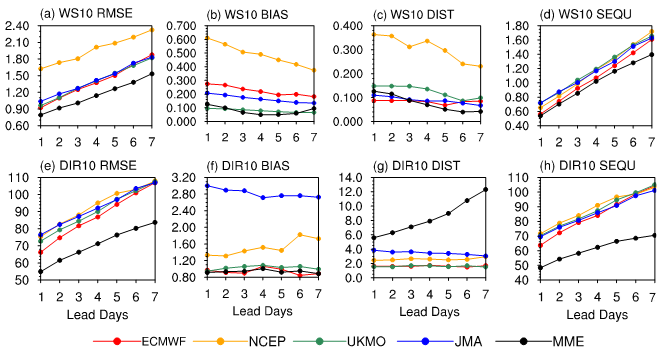
3.1. Evaluation of Multiple NWP Models and the MME

Figure 2 describes the regional averaged RMSE and TCC of ECMWF, NCEP, UKMO, JMA and MME for wind forecasts at the 10 m level over North China (NC) during a validation period of 1–7 lead days, including the meridional wind (U10), zonal wind (V10), wind speed (WS10) and wind direction (DIR10). Generally, multiple forecasts are characterized by consistent trends of increasing RMSE and decreasing TCC with growing lead times. The ECMWF shows the best performance, but with limited superiorities to UKMO and JMA, while the NCEP shows the lowest ability among the four NWP models. Specifically, the ECMWF features the lowest RMSEs and the highest TCCs at most lead times for all the elements. On the other hand, NCEP tends to show the highest RMSEs and the lowest TCCs, but it does not show much difference in comparison to other models in terms of WS10 forecasts. Furthermore, the MME is significantly superior to the individual NWP models, which is more evident for longer lead times. The RMSEs of the MME are lower than ECMWF by 0.3–0.5 m/s (12°–35°) for U10, V10 and WS10 (DIR10) for all lead times, and the MME shows TCCs of 0.1–0.15 higher than ECMWF for wind forecasts.
For assessments of the spatial distribution of forecast abilities for the NWP models and MME, with the lead time of 1 day taken as an example, Figure 3 describes the spatial distributions of RMSE for U10, V10, WS10 and DIR10 derived from ECMWF, NCEP and MME, which denote the best NWP model, the worst NWP model and the multimodel ensemble mean, respectively. In terms of U10 and V10, the lower RMSEs are continuously seen around central NC, whereas the highest RMSEs occur around northwestern NC. Meanwhile, the RMSEs of NCEP are higher than ECMWF over the whole area, and the advantages of MME to ECMWF are mainly reflected over the southwest NC. As for DIR10, the RMSE spatial distribution of ECMWF, NCEP and MME are generally consistent, with the largest RMSEs reaching up to 120° occurring at central NC, while the lowest RMSEs of lower than 40° are seen at northwestern NC. It is worth noting that the RMSEs are obviously lower over all regions in the MME than ECMWF.
In order to assess the wind forecasts at multiple isobaric surfaces, Figure 4 describes the regional averaged RMSE of U, V, WS and DIR at 500 hPa, 850 hPa, 700 hPa and 925 hPa, derived from ECMWF, NCEP, UKMO, JMA and MME over NC, with lead times of 1, 4 and 7 days taken as examples. Generally, the multiple forecasts are characterized by consistent trends of increasing RMSE (decreasing RMSE) for U, V and WS (DIR) with the rising height. Among them, the RMSE of U, V and WS show the highest growth rates between 925 hPa and 850 hPa, and the highest growth rate of DIR is seen between 700 hPa and 500 hPa. Furthermore, the ECMWF shows lower RMSE than the other NWP models at all isobaric surfaces, which is more evident at higher levels. The advantages of ECMWF diminish with increased lead times. Furthermore, the MME tends to show lower RMSE for U, V and WS (DIR) than ECMWF at all levels for all lead times, which is more obvious at higher (lower) levels for longer lead times.
To reveal the spatial distribution of wind forecast abilities at the isobaric surfaces for NWP models and the MME, Figure 5 describes the RMSE spatial distribution for U500, V500, WS500 and DIR500 derived from ECMWF, NCEP and MME, with the lead time of 1 day taken as an example. Generally, multiple forecasts show similar error distribution characteristics for U500, V500 and WS500. Specifically, the lower RMSEs are seen at central and northeastern NC, while the largest RMSEs occur at northwestern NC. Furthermore, NCEP shows limited forecast ability, with RMSEs reaching up to 2.2 m/s at most areas for U500, V500 and WS500, while the RMSEs of MME are mostly lower than 2 m/s. In terms of DIR500, the lowest RMSEs are seen at central NC for ECMWF, NCEP and MME, while the largest occurs at the northwestern and southern NC. Furthermore, the MME shows clear superiority to the two NWP models, with its RMSEs of lower than 60° for most areas.
To summarize, there is little difference in the performances of the four NWP models in terms of wind direction forecasts, but clear differences occur in the meridional wind, zonal wind and wind speed forecasts. The ECMWF shows general advantages over the other three at both 10 m and isobaric surfaces, which are more pronounced at isobaric surfaces. Furthermore, the forecast abilities of MME are superior to ECMWF for U, V, WS and DIR, which are more distinct at higher levels for longer lead times. It is worth noting that multiple forecasts manifest with the consistent trends of increasing (decreasing) RMSE for U, V and WS (DIR) with rising height. In addition, all the NWP models and MME tend to show higher forecast abilities at central NC, while they manifest with lower ability at northwestern NC for both ground and isobaric surfaces.

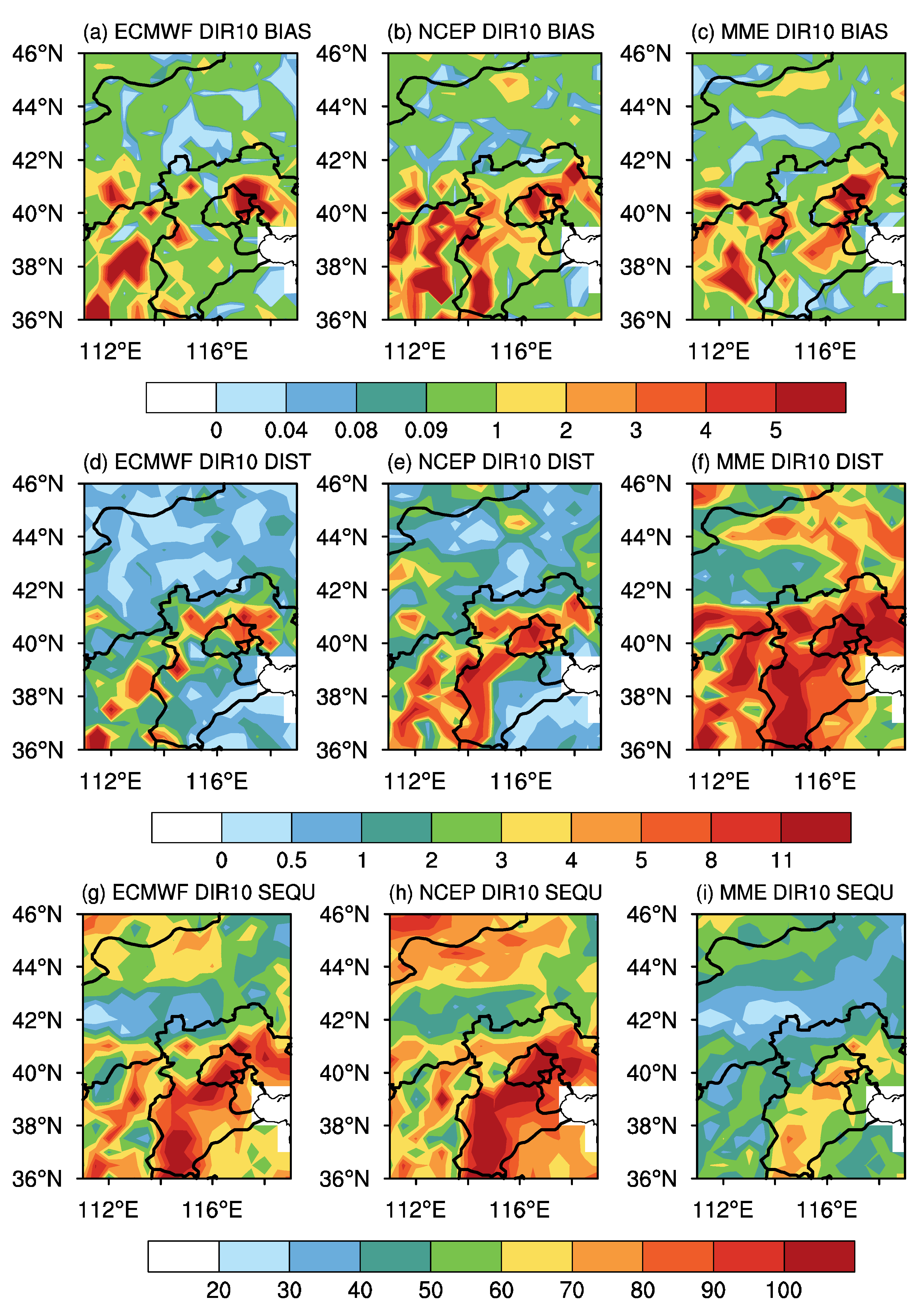
3.2. Error Decompositions of the Wind Forecasts

Although the forecast abilities of NWP models and MME have been assessed in Section 3.1 via metrics, including RMSE and TCC, they tend to provide overall ability scores and give little insight into which aspects of the models are good or bad. Thus, the error decomposition method is utilized in this section to diagnose the error sources of wind forecasts in NWP models, and to analyze which aspects of the forecasts are improved by the MME method.
Figure 6 describes the regional-averaged RMSE, the decomposed bias component (BIAS), the distribution error component (DIST) and the sequence error component (SEQU) of the 10 m wind speed (WS10) and direction (DIR10) over NC derived from ECMWF, NCEP, UKMO, JMA and MME for lead times of 1–7 days. Generally, SEQU is the main source of error for both WS10 and DIR10, and rises rapidly with increasing lead times. While BIAS and DIST account for a relatively small proportion of the total error and do not increase with growing lead times. It implies that the 10 m wind forecast errors are mainly attributed to the forecasts being ahead of (lagging behind) the observations. However, the deficiency of NCEP for WS10, compared with other NWP models, could mainly be attributed to the BIAS and DIST. Furthermore, the MME tends to generate lower SEQU than four NWP models for both WS10 and DIR10, which is more evident at longer lead times, while the BIAS and DIST of the MME could not show obvious superiority over the best NWP model.
To assess the spatial distributions of each error component, Figure 7 and Figure 8 describe the BIAS, DIST and SEQU spatial distributions derived from ECMWF, NCEP and MME over NC for WS10 and DIR10, respectively, with the lead time of 1 day taken as an example. Generally, multiple forecasts perform with consistent spatial distribution for both WS10 and DIR10. In terms of WS10, the largest BIASs and DISTs occur at central NC, while also characterized by the lowest SEQUs. In addition, the largest SEQUs of up to 1 m/s can be seen at northwestern and southeastern NC. Although MME is generally superior to ECMWF, its DISTs at northwestern NC are obviously higher than the ECMWF results. For DIR10, the largest BIASs, DISTs and SEQUs mainly occur at central NC, and the lowest DISTs and SEQUs can be seen at northwestern NC. Moreover, the MME shows lower SEQUs than the two NWP models over most areas, but the DISTs of the MME are generally higher than the two NWP models, which is more distinct at southeastern NC. It is worth noting that the higher BIASs and DISTs tend to occur in the regions characterized with high altitudes, while SEQUs are less affected. This implies that the BIASs and DISTs might be associated with the deficiency of NWP models in simulating real terrain.
Aiming at diagnoses of the wind forecast errors at the isobaric surface, Figure 9 shows the regional averaged RMSE and the components of BIAS, DIST and SEQU for WS500 and DIR500 over NC derived from the four NWP models and MME, with lead times of 1–7 days. Generally, the SEQU remains the main source of errors and they rise rapidly with increasing lead times for both WS500 and DIR500. Furthermore, the proportions accounted for by SEQU in total errors are higher than those in 10 m wind forecasts for both WS500 and DIR500. Unlike the 10 m wind forecasts, the insufficiency of the NCEP forecasts at 500 hPa could mainly be attributed to the SEQU. On the other hand, the MME is characterized by lower SEQU, along with higher BIAS and DIST, than all NWP models for the WS500, which is more evident at longer lead times.
Figure 10 and Figure 11 further describe the spatial distributions of BIAS, DIST and SEQU components derived from ECMWF, NCEP and MME over NC for WS500 and DIR500, with the lead time of 1 day taken as an example. In terms of WS500, the SEQUs of NCEP over most areas are greater than 2 m/s, which accounts for the overall insufficiency of the model. Furthermore, the MME shows generally lower SEQUs than the two NWP models, while the BIASs of MME at northern NC are higher than ECMWF and NCEP. For DIR500, the three forecast systems show generally consistent distributions, and the largest SEQUs are mainly distributed at northern NC. Furthermore, MME performs with the lower SEQUs than ECMWF and NCEP for most areas, but there are higher DISTs at northwestern NC in MME than the two models. In addition, MME could not produce overt improvements to ECMWF and NCEP in terms of the BIAS component.
In summary, the main source of wind forecast errors at both 10 m and isobaric surfaces is the SEQU component, which rises rapidly with increasing lead times. The proportions accounted for by SEQU in total errors at isobaric surfaces are higher than that at the 10 m level. The deficiency of NCEP at both 10 m and isobaric surfaces could mainly be attributed to the BIAS and SEQU terms, respectively. Furthermore, the MME tends to perform with lower SEQU than NWP models at both 10 m and isobaric surfaces, which is more distinct for longer lead times. However, the MME shows a slight deficiency in reducing BIAS and DIST. There are even higher DISTs for MME than NWP models, which are not included in detail here and require exploration in future work.

4. Conclusions and Discussion

In this study, the wind forecasts of 2020 derived from ECMWF, NCEP, UKMO and JMA over NC for lead times of 1–7 days at 10 m and isobaric surfaces (500 hPa, 700 hPa, 850 hPa and 925 hPa) were evaluated and the straightforward multimodel ensemble mean method (MME) was utilized to improve wind forecast abilities. Furthermore, the error decomposition method was also applied to diagnose the error sources of wind forecasts in NWP models and analyze which aspects of the forecasts were improved by the MME method. Associated results were obtained as follows.
Generally, there was little difference in the performances of the four NWP models in terms of wind direction forecasts, but evident differences occurred in the meridional wind, zonal wind and wind speed forecasts. The ECMWF showed general advantages over the other three NWP models at both 10 m and isobaric surfaces, which were more pronounced at isobaric surfaces. Furthermore, the forecast abilities of MME were superior to ECMWF for U, V, WS and DIR, which were more obvious at higher levels for longer lead times. It is worth noting that multiple forecasts manifested with the consistent trends of increasing (decreasing) RMSE for U, V, WS (DIR) with rising height. In addition, all the NWP models and MME tended to show higher forecast ability at central NC, while they manifested with lower ability at northwestern NC for both ground and isobaric surfaces.
The main source of wind forecast errors at both 10 m and isobaric surfaces was the SEQU component, which rose rapidly with increasing lead times. In addition, the proportions accounted by SEQU in total errors at isobaric surfaces were higher than that at the 10 m level. Furthermore, the deficiency of NCEP at the 10 m and isobaric surfaces could mainly be attributed to the BIAS and SEQU terms, respectively. Furthermore, the MME tended to perform with lower SEQU than NWP models at both 10 m and isobaric surfaces, which was more distinct for longer lead times. However, the MME showed slight deficiency in reducing BIAS and DIST, and there were even higher DISTs for the MME than the NWP models. These results not only provide an important reference for the use of wind NWP results in business departments and scientific research, but also in directing further improvement of NWPs in the future.
Moreover, according to the current study, higher BIASs and DISTs tended to occur at regions with high altitudes for wind forecasts at 10 m, which implied that the BIAS and DIST might be associated with the deficiency of the model in simulating the real terrain [48,49]. Thus, calibration methods incorporating geographic information should also be examined in the future [50,51]. On the other hand, the examined MME method is one of the most basic and straightforward multimodel ensemble methods, which assigns all models with the same role. Considering the deficiency of MME in reducing the BIAS and DIST of wind forecasts, the multimodel ensemble methods based on more complex algorithms assigning different weights for different models, including Kalman filter [52,53], object-based diagnosis [54] and deep learning methods [6,55], are also on the way to be utilized to further improve wind forecast ability. Furthermore, with the development of modern observation channels and technologies, observations are enriched and could be taken into consideration to assess and calibrate the model products in a more realistic way.

Author Contributions

Y.L. and X.Z. contributed to conception and design of the study. H.W., S.Z. and Y.Z. contributed to the analysis. H.Z., D.K. and C.H. organized the database. All authors contributed to manuscript revision, read, and approved the submitted version. All authors have read and agreed to the published version of the manuscript.

Funding

The study was jointly supported by the Collaboration Project of Urumqi Desert Meteorological Institute of China Meteorological Administration “Precipitation forecast based on machine learning”, the National Key R&D Program of China (Grant No. 2017YFC1502002), the Basic Research Fund of CAMS (Grant No. 2022Y027), the research project of Jiangsu Meteorological Bureau (Grant No. KQ202209).

Institutional Review Board Statement

Not applicable.

Informed Consent Statement

Not applicable.

Data Availability Statement

The forecast and observation data in this paper are publicly available. The datasets are obtained from the ECMWF archive in https://apps.ecmwf.int/datasets/, 1 August 2022.

Acknowledgments

The authors are grateful to ECMWF, NCEP, UKMO and JMA for their datasets.

Conflicts of Interest

The authors declare that the research was conducted in the absence of any commercial or financial relationships that could be construed as a potential conflict of interest.

References

  1. Sloughter, J.M.; Gneiting, T.; Raftery, A.E. Probabilistic wind vector forecasting using ensembles and Bayesian model averaging. Mon. Weather. Rev. 2013, 141, 2107–2119. [Google Scholar] [CrossRef] [Green Version]
  2. Adeyeye, K.; Ijumba, N.; Colton, J. Exploring the environmental and economic impacts of wind energy: A cost-benefit perspective. Int. J. Sustain. Dev. World Ecol. 2020, 27, 718–731. [Google Scholar] [CrossRef]
  3. Wen, Y.; Chen, Z. Study on the Estimation of Designed Wind Speed for Jingyue Yangtze River Highway Bridge. J. Wuhan Univ. Technol. Transp. Sci. Eng. 2010, 34, 306–309. [Google Scholar]
  4. Wynnyk, C.M. Wind analysis in aviation applications. In Proceedings of the 2012 IEEE/AIAA 31st Digital Avionics Systems Conference (DASC), Williamsburg, VA, USA, 14–18 October 2012; pp. 5C2-1–5C2-10. [Google Scholar]
  5. Wilczak, J.; Finley, C.; Freedman, J.; Cline, J.; Bianco, L.; Olson, J.; Djalalova, I.; Sheridan, L.; Ahlstrom, M.; Manobianco, J.; et al. The Wind Forecast Improvement Project (WFIP): A public—Private partnership addressing wind energy forecast needs. Bull. Am. Meteorol. Soc. 2015, 96, 1699–1718. [Google Scholar] [CrossRef]
  6. Veldkamp, S.; Whan, K.; Dirksen, S. Statistical postprocessing of wind speed forecasts using convolutional neural networks. Mon. Weather. Rev. 2021, 149, 1141–1152. [Google Scholar] [CrossRef]
  7. Zhu, S.; Remedio, A.R.C.; Sein, D.V.; Sielmann, F.; Ge, F.; Xu, J.; Peng, T.; Jacob, D.; Fraedrich, K.; Zhi, X. Added value of the regionally coupled model ROM in the East Asian summer monsoon modeling. Theor. Appl. Climatol. 2020, 140, 375–387. [Google Scholar] [CrossRef] [Green Version]
  8. Bauer, P.; Thorpe, A.; Brunet, G. The quiet revolution of numerical weather prediction. Nature 2015, 525, 47–55. [Google Scholar] [CrossRef]
  9. Zhu, S.; Ge, F.; Sielmann, F.; Pan, M.; Fraedrich, K.; Remedio, A.R.C.; Sein, D.V.; Jacob, D.; Wang, H.; Zhi, X. Seasonal temperature response over the Indochina Peninsula to a worst-case high-emission forcing: A study with the regionally coupled model ROM. Theor. Appl. Climatol. 2020, 142, 613–622. [Google Scholar] [CrossRef]
  10. Bengtsson, L.; Andrae, U.; Aspelien, T.; Batrak, Y.; Calvo, J.; de Rooy, W.; Gleeson, E.; Hansen-Sass, B.; Homleid, M.; Hortal, M.; et al. The HARMONIE–AROME model configuration in the ALADIN–HIRLAM NWP system. Mon. Weather. Rev. 2017, 145, 1919–1935. [Google Scholar] [CrossRef]
  11. Zhang, L.; Kim, T.; Yang, T.; Hong, Y.; Zhu, Q. Evaluation of Subseasonal-to-Seasonal (S2S) precipitation forecast from the North American Multi-Model ensemble phase II (NMME-2) over the contiguous US. J. Hydrol. 2021, 603, 127058. [Google Scholar] [CrossRef]
  12. Lyu, Y.; Zhu, S.; Zhi, X.; Dong, F.; Zhu, C.; Ji, L.; Fan, Y. Subseasonal forecasts of precipitation over Maritime Continent in boreal summer and the sources of predictability. Front. Earth Sci. 2022, 10, 970791. [Google Scholar] [CrossRef]
  13. Louvet, S.; Sultan, B.; Janicot, S.; Kamsu-Tamo, P.H.; Ndiaye, O. Evaluation of TIGGE precipitation forecasts over West Africa at intraseasonal timescale. Clim. Dyn. 2016, 47, 31–47. [Google Scholar] [CrossRef]
  14. Lorenz, E.N. Atmospheric predictability as revealed by naturally occurring analogues. J. Atmos. Sci. 1969, 26, 636–646. [Google Scholar] [CrossRef]
  15. Zhang, H.; Chen, M.; Fan, S. Study on the construction of initial condition perturbations for the regional ensemble prediction system of North China. Atmosphere 2019, 10, 87. [Google Scholar] [CrossRef] [Green Version]
  16. Schulz, B.; Lerch, S. Machine learning methods for postprocessing ensemble forecasts of wind gusts: A systematic comparison. Mon. Weather. Rev. 2022, 150, 235–257. [Google Scholar] [CrossRef]
  17. Zhu, Y.; Luo, Y. Precipitation calibration based on the frequency-matching method. Weather. Forecast. 2015, 30, 1109–1124. [Google Scholar] [CrossRef]
  18. Guo, R.; Yu, H.; Yu, Z.; Tang, J.; Bai, L. Application of the frequency-matching method in the probability forecast of landfalling typhoon rainfall. Front. Earth Sci. 2022, 16, 52–63. [Google Scholar] [CrossRef]
  19. Hacker, J.P.; Rife, D.L. A practical approach to sequential estimation of systematic error on near-surface mesoscale grids. Weather. Forecast. 2007, 22, 1257–1273. [Google Scholar] [CrossRef]
  20. Kim, H.M.; Ham, Y.G.; Scaife, A.A. Improvement of initialized decadal predictions over the North Pacific Ocean by systematic anomaly pattern correction. J. Clim. 2014, 27, 5148–5162. [Google Scholar] [CrossRef]
  21. Lyu, Y.; Zhi, X.; Zhu, S.; Fan, Y.; Pan, M. Statistical calibrations of surface air temperature forecasts over east Asia using pattern projection methods. Weather. Forecast. 2021, 36, 1661–1674. [Google Scholar] [CrossRef]
  22. Belorid, M.; Kim, K.R.; Cho, C. Bias Correction of short-range ensemble forecasts of daily maximum temperature using decaying average. Asia Pac. J. Atmos. Sci. 2020, 56, 503–514. [Google Scholar] [CrossRef]
  23. Han, K.; Choi, J.T.; Kim, C. Comparison of statistical post-processing methods for probabilistic wind speed forecasting. Asia Pac. J. Atmos. Sci. 2018, 54, 91–101. [Google Scholar] [CrossRef]
  24. Krishnamurti, T.N.; Kishtawal, C.M.; LaRow, T.E.; Bachiochi, D.R.; Zhang, Z.; Williford, C.E.; Gadgil, S.; Surendran, S. Improved weather and seasonal climate forecasts from multimodel superensemble. Science 1999, 285, 1548–1550. [Google Scholar] [CrossRef] [Green Version]
  25. Jun, S.; Kang, N.Y.; Lee, W.; Chung, Y. An alternative multi-model ensemble forecast for tropical cyclone tracks in the western North Pacific. Atmosphere 2017, 8, 174. [Google Scholar] [CrossRef] [Green Version]
  26. Ji, L.; Zhi, X.; Zhu, S.; Fraedrich, K. Probabilistic precipitation forecasting over East Asia using Bayesian model averaging. Weather. Forecast. 2019, 34, 377–392. [Google Scholar] [CrossRef]
  27. Zhang, L.; Zhi, X.F. Multimodel consensus forecasting of low temperature and icy weather over central and southern China in early 2008. J. Trop. Meteorol. 2015, 21, 67–75. [Google Scholar]
  28. Krishnamurti, T.N.; Kishtawal, C.M.; Zhang, Z.; LaRow, T.; Bachiochi, D.; Williford, E.; Gadgil, S.; Surendran, S. Multimodel ensemble forecasts for weather and seasonal climate. J. Clim. 2000, 13, 4196–4216. [Google Scholar] [CrossRef]
  29. Krishnamurti, T.N.; Kumar, V.; Simon, A.; Bhardwaj, A.; Ghosh, T.; Ross, R. A review of multimodel superensemble forecasting for weather, seasonal climate, and hurricanes. Rev. Geophys. 2016, 54, 336–377. [Google Scholar] [CrossRef]
  30. Zhi, X.; Qi, H.; Bai, Y.; Lin, C. A comparison of three kinds of multimodel ensemble forecast techniques based on the TIGGE data. Acta Meteorol. Sin. 2012, 26, 41–51. [Google Scholar] [CrossRef]
  31. Koh, T.Y.; Wang, S.; Bhatt, B.C. A diagnostic suite to assess NWP performance. J. Geophys. Res. Atmos. 2012, 117, D13. [Google Scholar] [CrossRef]
  32. Gupta, H.V.; Kling, H.; Yilmaz, K.K.; Martinez, G.F. Decomposition of the mean squared error and NSE performance criteria: Implications for improving hydrological modelling. J. Hydrol. 2009, 377, 80–91. [Google Scholar] [CrossRef] [Green Version]
  33. Zhang, Y.; Ye, A.; Nguyen, P.; Analui, B.; Sorooshian, S.; Hsu, K. New insights into error decomposition for precipitation products. Geophys. Res. Lett. 2021, 48, e2021GL094092. [Google Scholar] [CrossRef]
  34. Sinha, T.; Sankarasubramanian, A.; Mazrooei, A. Decomposition of sources of errors in monthly to seasonal streamflow forecasts in a rainfall–runoff regime. J. Hydrometeorol. 2014, 15, 2470–2483. [Google Scholar] [CrossRef] [Green Version]
  35. Mazrooei, A.; Sinha, T.; Sankarasubramanian, A.; Kumar, S.; Peters-Lidard, C.D. Decomposition of sources of errors in seasonal streamflow forecasting over the US Sunbelt. J. Geophys. Res. Atmos. 2015, 120, 11,809–11,825. [Google Scholar] [CrossRef]
  36. Murphy, A.H. Skill scores based on the mean square error and their relationships to the correlationcoefficient. Mon. Weather. Rev. 1988, 116, 2417–2424. [Google Scholar] [CrossRef]
  37. Geman, S.; Bienenstock, E.; Doursat, R. Neural networks and the bias/variance dilemma. Neural Comput. 1992, 4, 1–58. [Google Scholar] [CrossRef]
  38. Hodson, T.O.; Over, T.M.; Foks, S.S. Mean squared error, deconstructed. J. Adv. Model. Earth Syst. 2021, 13, e2021MS002681. [Google Scholar] [CrossRef]
  39. Zhang, L.; Zhou, T.; Wu, P.; Chen, X. Potential predictability of North China summer drought. J. Clim. 2019, 32, 7247–7264. [Google Scholar] [CrossRef]
  40. Liu, Y.; Pan, Z.; Zhuang, Q.; Miralles, D.G.; Teuling, A.J.; Zhang, T.; An, P.; Dong, Z.; Zhang, J.; He, D.; et al. Agriculture intensifies soil moisture decline in Northern China. Sci. Rep. 2015, 5, 11261. [Google Scholar] [CrossRef] [Green Version]
  41. Hersbach, H.; Bell, B.; Berrisford, P.; Hirahara, S.; Horányi, A.; Muñoz-Sabater, J.; Nicolas, J.; Peubey, C.; Radu, R.; Schepers, D.; et al. The ERA5 global reanalysis. Q. J. R. Meteorol. Soc. 2020, 146, 1999–2049. [Google Scholar] [CrossRef]
  42. Olauson, J. ERA5: The new champion of wind power modelling? Renew. Energy 2018, 126, 322–331. [Google Scholar] [CrossRef] [Green Version]
  43. Hamill, T.M.; Hagedorn, R.; Whitaker, J.S. Probabilistic forecast calibration using ECMWF and GFS ensemble reforecasts. Part II: Precipitation. Mon. Weather. Rev. 2008, 136, 2620–2632. [Google Scholar] [CrossRef]
  44. Tarek, M.; Brissette, F.P.; Arsenault, R. Large-scale analysis of global gridded precipitation and temperature datasets for climate change impact studies. J. Hydrometeorol. 2020, 21, 2623–2640. [Google Scholar] [CrossRef]
  45. Graham, R.M.; Hudson, S.R.; Maturilli, M. Improved performance of ERA5 in Arctic gateway relative to four global atmospheric reanalyses. Geophys. Res. Lett. 2019, 46, 6138–6147. [Google Scholar] [CrossRef] [Green Version]
  46. Zhang, L.; Ma, X.; Zhu, S.; Guo, Z.; Zhi, X.; Chen, C. Analyses and applications of the precursor signals of a kind of warm sector heavy rainfall over the coast of Guangdong, China. Atmos. Res. 2022, 280, 106425. [Google Scholar] [CrossRef]
  47. Hagedorn, R.; Buizza, R.; Hamill, T.M.; Leutbecher, M.; Palmer, T.N. Comparing TIGGE multimodel forecasts with reforecast-calibrated ECMWF ensemble forecasts. Q. J. R. Meteorol. Soc. 2012, 138, 1814–1827. [Google Scholar] [CrossRef]
  48. Bao, X.; Zhang, F.; Sun, J. Diurnal variations of warm-season precipitation east of the Tibetan Plateau over China. Mon. Weather. Rev. 2011, 139, 2790–2810. [Google Scholar] [CrossRef]
  49. Bromwich, D.H.; Cullather, R.I.; Grumbine, R.W. An assessment of the NCEP operational global spectral model forecasts and analyses for Antarctica during FROST. Weather. Forecast. 1999, 14, 835–850. [Google Scholar] [CrossRef]
  50. Steinacker, R.; Ratheiser, M.; Bica, B.; Chimani, B.; Dorninger, M.; Gepp, W.; Lotteraner, C.; Schneider, S.; Tschannett, S. A mesoscale data analysis and downscaling method over complex terrain. Mon. Weather. Rev. 2006, 134, 2758–2771. [Google Scholar] [CrossRef] [Green Version]
  51. Han, L.; Chen, M.; Chen, K.; Chen, H.; Zhang, Y.; Lu, B.; Song, L.; Qin, R. A deep learning method for bias correction of ECMWF 24–240 h forecasts. Adv. Atmos. Sci. 2021, 38, 1444–1459. [Google Scholar] [CrossRef]
  52. Zhu, S.; Zhi, X.; Ge, F.; Fan, Y.; Zhang, L.; Gao, J. Subseasonal forecast of surface air temperature using superensemble approaches: Experiments over Northeast Asia for 2018. Weather. Forecast. 2021, 36, 39–51. [Google Scholar] [CrossRef]
  53. He, C.; Zhi, X.; You, Q.; Song, B.; Fraedrich, K. Multi-model ensemble forecasts of tropical cyclones in 2010 and 2011 based on the Kalman Filter method. Meteorol. Atmos. Phys. 2015, 127, 467–479. [Google Scholar] [CrossRef]
  54. Ji, L.; Zhi, X.; Simmer, C.; Zhu, S.; Ji, Y. Multimodel ensemble forecasts of precipitation based on an object-based diagnostic evaluation. Mon. Weather. Rev. 2020, 148, 2591–2606. [Google Scholar] [CrossRef]
  55. Peng, T.; Zhi, X.; Ji, Y.; Ji, L.; Tian, Y. Prediction skill of extended range 2-m maximum air temperature probabilistic forecasts using machine learning post-processing methods. Atmosphere 2020, 11, 823. [Google Scholar] [CrossRef]
Figure 1. Topography (m) of North China (marked region) and its surrounding area.
Atmosphere 13 01652 g001
Figure 2. Variations in RMSE and TCC of U10, V10, WS10 and DIR10, at lead times of 1–7 days derived from ECMWF, NCEP, UKMO, JMA and MMA averaged over North China.
Atmosphere 13 01652 g002
Figure 3. Spatial distributions of RMSEs for U10, V10, WS10 and DIR10 with a lead time of 1 day derived from ECMWF, NCEP and MME.
Atmosphere 13 01652 g003
Figure 4. Variations in RMSE for U, V, WS and DIR at isobaric surfaces (500 hPa, 700 hPa, 850 hPa, 925 hPa) for lead times of 1–7 days, derived from ECMWF, NCEP, UKMO, JMA and MMA, averaged over North China.
Atmosphere 13 01652 g004
Figure 5. Spatial distributions of RMSEs for U500, V500, WS500 and DIR500 with a lead time of 1 day derived from ECMWF, NCEP and MME.
Atmosphere 13 01652 g005
Figure 6. Variations in RMSE, decomposed BIAS, DIST and SEQU for WS10 and DIR10 at lead times of 1–7 days derived from ECMWF, NCEP, UKMO, JMA and MMA, averaged over North China.
Atmosphere 13 01652 g006
Figure 7. Spatial distributions of decomposed BIAS, DIST and SEQU for WS10 with a lead time of 1 day derived from ECMWF, NCEP and MME.
Atmosphere 13 01652 g007
Figure 8. Spatial distributions of decomposed BIAS, DIST and SEQU for DIR10 with a lead time of 1 day derived from ECMWF, NCEP and MME.
Atmosphere 13 01652 g008
Figure 9. Variations in RMSE, decomposed BIAS, DIST and SEQU for WS500 and DIR500 at lead times of 1–7 days derived from ECMWF, NCEP, UKMO, JMA and MMA, averaged over North China.
Atmosphere 13 01652 g009
Figure 10. Spatial distributions of decomposed BIAS, DIST and SEQU for WS500 with a lead time of 1 day derived from ECMWF, NCEP and MME.
Atmosphere 13 01652 g010
Figure 11. Spatial distributions of decomposed BIAS, DIST and SEQU for DIR500 with a lead time of 1 day derived from ECMWF, NCEP and MME.
Atmosphere 13 01652 g011
Publisher’s Note: MDPI stays neutral with regard to jurisdictional claims in published maps and institutional affiliations.

