
Regime Changes in Atmospheric Moisture under Climate Change

Abstract
:1. Introduction
2. Materials and Methods
3. Results
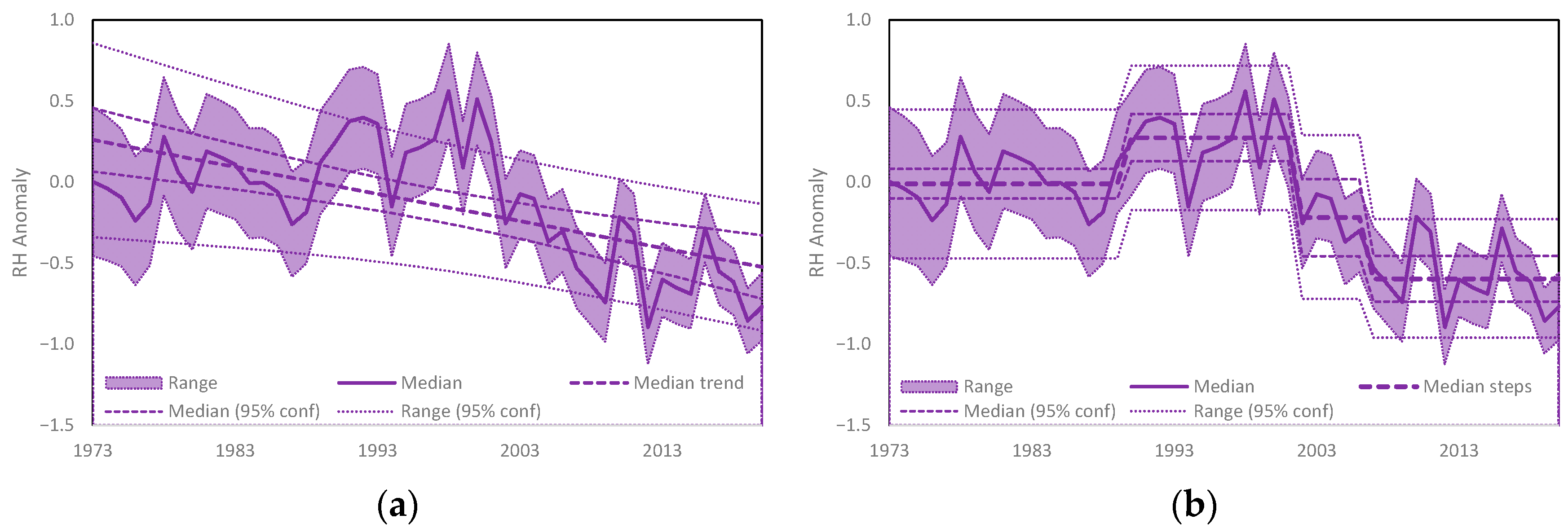
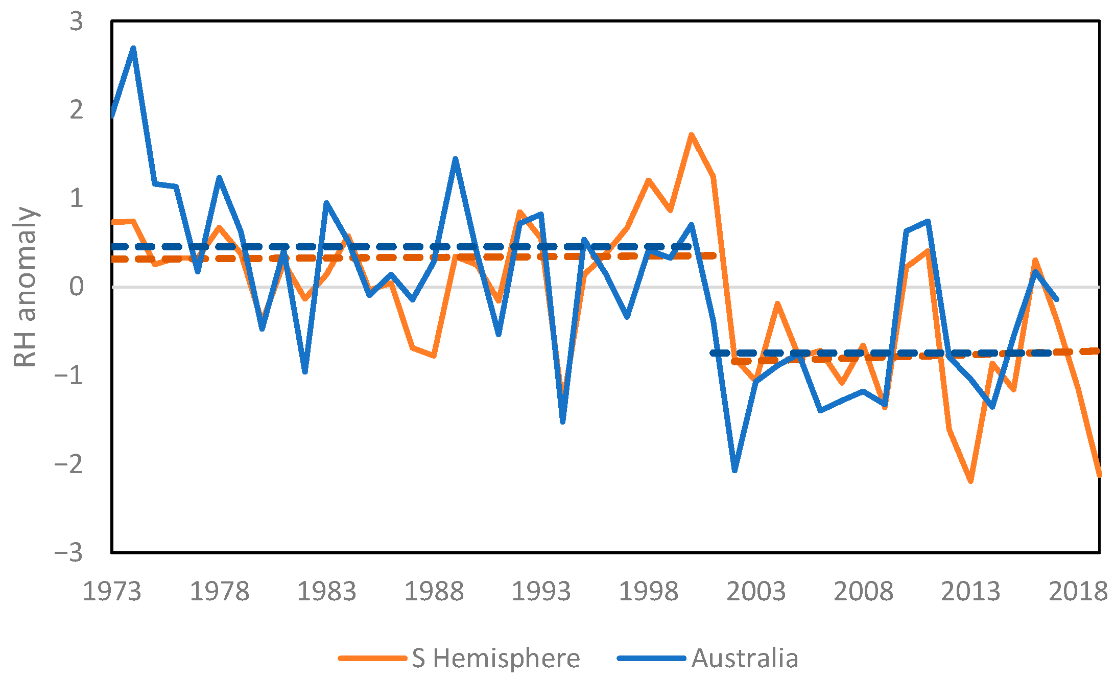
3.1. Observations
Exploring Uncertainty
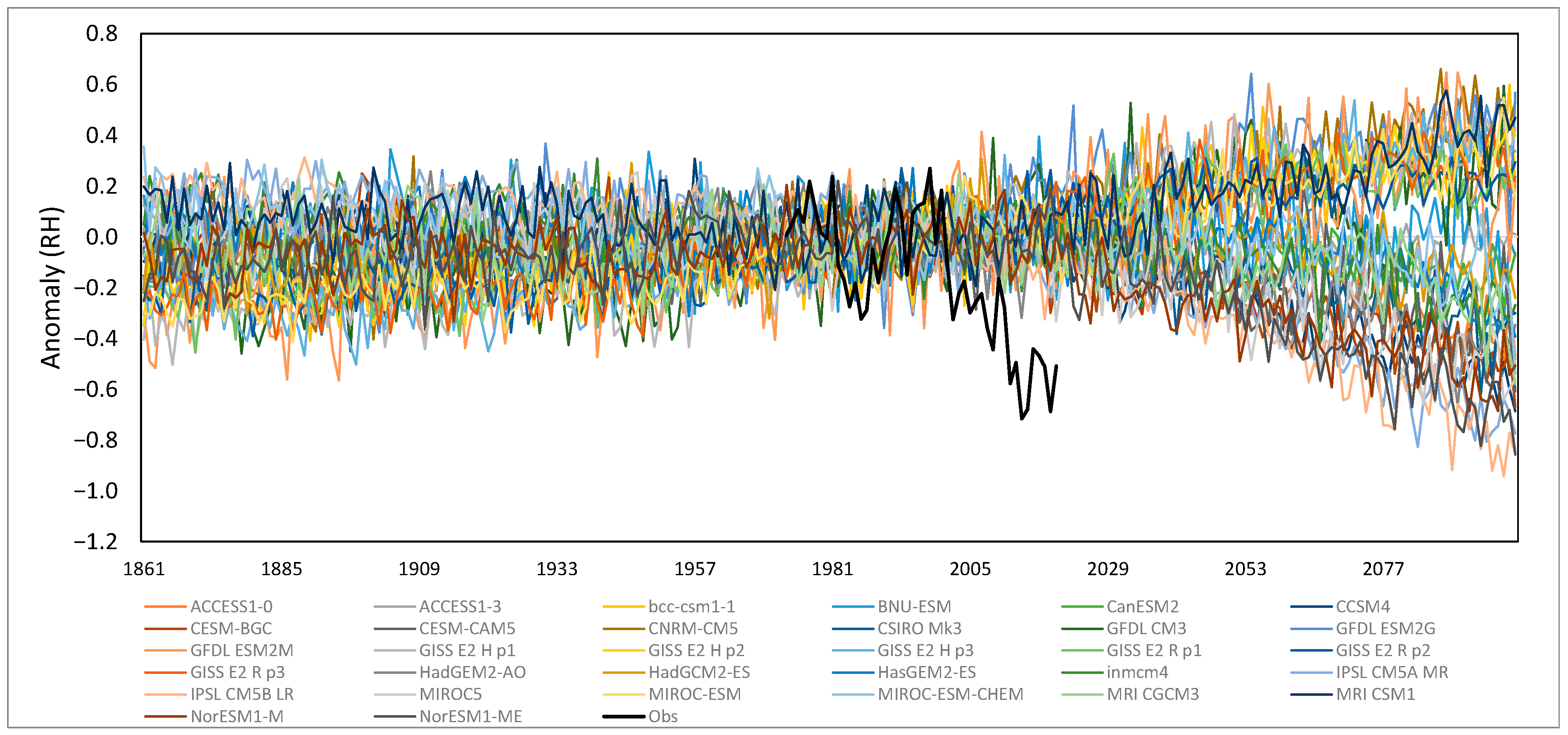
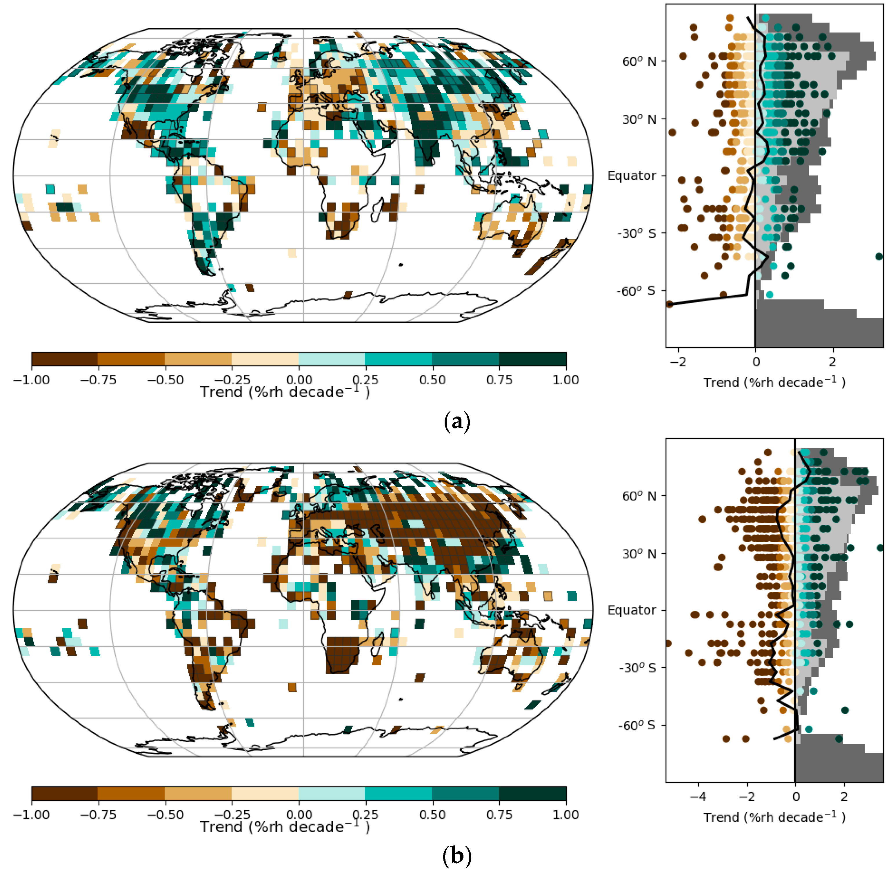
3.2. Comparison with Climate Models
3.3. Attribution
Other Studies
3.4. Impacts
4. Discussion
4.1. Attribution Methods
4.2. Contributing Processes and Mechanisms
5. Conclusions
Supplementary Materials
Author Contributions
Funding
Institutional Review Board Statement
Informed Consent Statement
Data Availability Statement
Acknowledgments
Conflicts of Interest
References
- Belolipetsky, P.V.; Bartsev, S.; Ivanova, Y.; Saltykov, M. Hidden staircase signal in recent climate dynamic. Asia-Pac. J. Atmos. Sci. 2015, 51, 323–330. [Google Scholar] [CrossRef]
- Jones, R.N.; Young, C.K.; Handmer, J.; Keating, A.; Mekala, G.D.; Sheehan, P. Valuing Adaptation under Rapid Change; National Climate Change Adaptation Research Facility: Gold Coast, QLD, Australia, 2013; p. 182. [Google Scholar]
- Reid, P.C.; Beaugrand, G. Global synchrony of an accelerating rise in sea surface temperature. J. Mar. Biol. Assoc. UK 2012, 92, 1435–1450. [Google Scholar] [CrossRef]
- Jones, R.N. Detecting and attributing nonlinear anthropogenic regional warming in southeastern Australia. J. Geophys. Res. 2012, 117, D04105. [Google Scholar] [CrossRef]
- Belolipetsky, P.V. The Shifts Hypothesis—An alternative view of global climate change. arXiv 2014, arXiv:1406.5805. [Google Scholar]
- Reid, P.C.; Hari, R.E.; Beaugrand, G.; Livingstone, D.M.; Marty, C.; Straile, D.; Barichivich, J.; Goberville, E.; Adrian, R.; Aono, Y. Global impacts of the 1980s regime shift. Global Change Biol. 2016, 22, 682–703. [Google Scholar] [CrossRef] [PubMed]
- Jones, R.N.; Ricketts, J.H. Reconciling the signal and noise of atmospheric warming on decadal timescales. Earth Syst. Dyn. 2017, 8, 177–210. [Google Scholar] [CrossRef]
- Mayo, D.G. Statistical Inference as Severe Testing; Cambridge University Press: Cambridge, UK, 2018; p. 486. [Google Scholar]
- IPCC. Climate Change 2021: The Physical Science Basis. Contribution of Working Group I to the Sixth Assessment Report of the Intergovernmental Panel on Climate Change; Masson-Delmotte, V., Zhai, P., Priani, A., Connors, S., Péan, C., Berger, S., Eds.; Cambridge University Press: Cambridge, UK, 2021.
- Jones, R.N.; Ricketts, J.H. The Pacific Ocean heat engine. Earth Syst. Dyn. Discuss. 2021, 2021, 1–47. [Google Scholar] [CrossRef]
- Pall, P.; Allen, M.; Stone, D.A. Testing the Clausius–Clapeyron constraint on changes in extreme precipitation under CO2 warming. Clim. Dyn. 2007, 28, 351–363. [Google Scholar] [CrossRef]
- O’Gorman, P.A.; Muller, C.J. How closely do changes in surface and column water vapor follow Clausius–Clapeyron scaling in climate change simulations? Environ. Res. Lett. 2010, 5, 025207. [Google Scholar] [CrossRef]
- Kim, S.; Sharma, A.; Wasko, C.; Nathan, R. Linking total precipitable water to precipitation extremes globally. Earth’s Future 2022, 10, e2021EF002473. [Google Scholar] [CrossRef]
- Parker, T.; Gallant, A.; Hobbins, M.; Hoffmann, D. Flash drought in Australia and its relationship to evaporative demand. Environ. Res. Lett. 2021, 16, 064033. [Google Scholar] [CrossRef]
- Otkin, J.A.; Zhong, Y.; Hunt, E.D.; Christian, J.I.; Basara, J.B.; Nguyen, H.; Wheeler, M.C.; Ford, T.W.; Hoell, A.; Svoboda, M. Development of a flash drought intensity index. Atmosphere 2021, 12, 741. [Google Scholar] [CrossRef]
- Beer, T.; Williams, A. Estimating Australian forest fire danger under conditions of doubled carbon dioxide concentrations. Clim. Change 1995, 29, 169–188. [Google Scholar] [CrossRef]
- Rodriguez-Iturbe, I. Ecohydrology: A hydrologic perspective of climate-soil-vegetation dynamies. Water Resour. Res. 2000, 36, 3–9. [Google Scholar] [CrossRef]
- Allan, R.; Barlow, M.; Byrne, M.P.; Cherchi, A.; Douville, H.; Fowler, H.J.; Gan, T.Y.; Pendergrass, A.G.; Rosenfeld, D.; Swann, A.L. Advances in understanding large-scale responses of the water cycle to climate change. Ann. N. Y. Acad. Sci. 2020, 1472, 49–75. [Google Scholar] [CrossRef]
- Davis, R.E.; McGregor, G.R.; Enfield, K.B. Humidity: A review and primer on atmospheric moisture and human health. Environ. Res. 2016, 144, 106–116. [Google Scholar] [CrossRef] [PubMed]
- Gimeno, L.; Dominguez, F.; Nieto, R.; Trigo, R.; Drumond, A.; Reason, C.J.; Taschetto, A.S.; Ramos, A.M.; RameshKumar, M.; Marengo, J. Major mechanisms of atmospheric moisture transport and their role in extreme precipitation events. Annu. Rev. Environ. Resour. 2016, 41, 117–141. [Google Scholar] [CrossRef]
- Dai, A. Drought under global warming: A review. Wiley Interdiscip. Rev. Clim. Change 2011, 2, 45–65. [Google Scholar] [CrossRef]
- Maronna, R.; Yohai, V.J. A bivariate test for the detection of a systematic change in mean. J. Am. Stat. Assoc. 1978, 73, 640–645. [Google Scholar] [CrossRef]
- Ricketts, J.H. A probabilistic approach to climate regime shift detection based on Maronna’s bivariate test. In Proceedings of the 21st International Congress on Modelling and Simulation (MODSIM2015), Gold Coast, QLD, Australia, 29 November–4 December 2015; pp. 1310–1316. [Google Scholar]
- Ricketts, J.H. Understanding the Nature of Abrupt Decadal Shifts in a Changing Climate. Ph.D. Thesis, Victoria University, Melbourne, VIC, Australia, 2019. [Google Scholar]
- Zaiontz, C. Real Statistics Resource Pack, v6.0. 2018. Available online: www.real-statistics.com (accessed on 29 September 2019).
- Willett, K.; Dunn, R.; Thorne, P.; Bell, S.; De Podesta, M.; Parker, D.; Jones, P.; Williams, C., Jr. HadISDH land surface multi-variable humidity and temperature record for climate monitoring. Clim. Past 2014, 10, 1986–2006. [Google Scholar] [CrossRef]
- Smith, A.; Lott, N.; Vose, R. The integrated surface database: Recent developments and partnerships. Bull. Am. Meteorol. Soc. 2011, 92, 704–708. [Google Scholar] [CrossRef] [Green Version]
- Willett, K.M.; Dunn, R.J.; Kennedy, J.J.; Berry, D.I. Development of the HadISDH marine humidity climate monitoring dataset. Earth Syst. Sci. Data 2020, 12, 2853–2880. [Google Scholar] [CrossRef]
- Freeman, E.; Woodruff, S.D.; Worley, S.J.; Lubker, S.J.; Kent, E.C.; Angel, W.E.; Berry, D.I.; Brohan, P.; Eastman, R.; Gates, L. ICOADS Release 3.0: A major update to the historical marine climate record. Int. J. Climatol. 2017, 37, 2211–2232. [Google Scholar] [CrossRef]
- Willett, K.M.; Williams, C.N., Jr.; Dunn, R.J.; Thorne, P.W.; Bell, S.; de Podesta, M.; Jones, P.D.; Parker, D.E. HadISDH: An updateable land surface specific humidity product for climate monitoring. Clim. Past. 2013, 9, 657–677. [Google Scholar] [CrossRef]
- Byrne, M.P.; O’Gorman, P.A. Trends in continental temperature and humidity directly linked to ocean warming. Proc. Natl. Acad. Sci. USA 2018, 115, 4863–4868. [Google Scholar] [CrossRef]
- Vicente-Serrano, S.M.; Nieto, R.; Gimeno, L.; Azorin-Molina, C.; Drumond, A.; El Kenawy, A.; Dominguez-Castro, F.; Tomas-Burguera, M.; Peña-Gallardo, M. Recent changes of relative humidity: Regional connections with land and ocean processes. Earth Syst. Dyn. 2018, 9, 915–937. [Google Scholar] [CrossRef]
- Dunn, R.J.; Willett, K.M.; Ciavarella, A.; Stott, P.A. Comparison of land surface humidity between observations and CMIP5 models. Earth Syst. Dyn. 2017, 8, 719. [Google Scholar] [CrossRef]
- Sun, C.; Kucharski, F.; Li, J.; Jin, F.-F.; Kang, I.-S.; Ding, R. Western tropical Pacific multidecadal variability forced by the Atlantic multidecadal oscillation. Nat. Commun. 2017, 8, 1–10. [Google Scholar] [CrossRef]
- University of East Anglia Climatic Research Unit; Harris, I.C.; Jones, P.D. CRU TS4.03: Climatic Research Unit (CRU) Time-Series (TS) Version 4.03 of High-Resolution Gridded Data of Month-By-Month Variation in Climate (Jan. 1901–Dec. 2018), Centre for Environmental Data Analysis. 2020. Available online: https://catalogue.ceda.ac.uk/uuid/10d3e3640f004c578403419aac167d82 (accessed on 20 April 2020).
- Thorne, P.W.; Parker, D.E.; Christy, J.R.; Mears, C.A. Uncertainties in Climate Trends: Lessons from Upper-Air Temperature Records. Bull. Am. Meteorol. Soc. 2005, 86, 1437–1442. [Google Scholar] [CrossRef]
- Loeb, N.G.; Johnson, G.C.; Thorsen, T.J.; Lyman, J.M.; Rose, F.G.; Kato, S. Satellite and ocean data reveal marked increase in Earth’s heating rate. Geophys. Res. Lett. 2021, 48, e2021GL093047. [Google Scholar] [CrossRef]
- Thomson, A.; Calvin, K.; Smith, S.; Kyle, G.P.; Volke, A.; Patel, P.; Delgado-Arias, S.; Bond-Lamberty, B.; Wise, M.; Clarke, L.; et al. RCP4.5: A pathway for stabilization of radiative forcing by 2100. Clim. Change 2011, 109, 77–94. [Google Scholar] [CrossRef] [Green Version]
- Douville, H.; Plazzotta, M. Midlatitude summer drying: An underestimated threat in CMIP5 models? Geophys. Res. Lett. 2017, 44, 9967–9975. [Google Scholar] [CrossRef]
- Gulev, S.K.; Thorne, P.W.; Ahn, J.; Dentener, F.J.; Domingues, C.M.; Gerland, S.; Gong, D.; Kaufman, D.S.; Nnamchi, H.C.; Quaas, J.; et al. Changing state of the climate system. In Climate Change 2021: Contribution of Working Group I to the Sixth Assessment Report of the Intergovernmental Panel on Climate Change; Masson-Delmotte, V., Zhai, P., Pirani, A., Connors, S.L., Péan, C., Berger, S., Caud, N., Chen, Y., Goldfarb, L., Gomis, M.I., et al., Eds.; Cambridge University Press: Cambridge, UK, 2021; pp. 287–422. [Google Scholar]
- Hartmann, D.L.; Tank, A.M.G.K.; Rusticucci, M.; Alexander, L.V.; Brönnimann, S.; Charabi, Y.; Dentener, F.J.; Dlugokencky, E.J.; Easterling, D.R.; Kaplan, A.; et al. Observations: Atmosphere and Surface. In Climate Change 2013: The Physical Science Basis. Contribution of Working Group I to the Fifth Assessment Report of the Intergovernmental Panel on Climate Change; Stocker, T.F., Qin, D., Plattner, G.-K., Tignor, M., Allen, S.K., Boschung, J., Nauels, A., Xia, Y., Bex, V., Midgley, P.M., Eds.; Cambridge University Press: Cambridge, UK; New York, NY, USA, 2013; pp. 159–254. [Google Scholar]
- Boer, G. The ratio of land to ocean temperature change under global warming. Clim. Dyn. 2011, 37, 2253–2270. [Google Scholar] [CrossRef]
- Dommenget, D. The Ocean’s Role in Continental Climate Variability and Change. J. Clim. 2009, 22, 4939–4952. [Google Scholar] [CrossRef]
- Gimeno, L.; Drumond, A.; Nieto, R.; Trigo, R.M.; Stohl, A. On the origin of continental precipitation. Geophys. Res. Lett. 2010, 37. [Google Scholar] [CrossRef]
- Gimeno, L.; Stohl, A.; Trigo, R.M.; Dominguez, F.; Yoshimura, K.; Yu, L.; Drumond, A.; Durán-Quesada, A.M.; Nieto, R. Oceanic and terrestrial sources of continental precipitation. Rev. Geophys. 2012, 50. [Google Scholar] [CrossRef]
- Van der Ent, R.J.; Savenije, H.H.; Schaefli, B.; Steele-Dunne, S.C. Origin and fate of atmospheric moisture over continents. Water Resour. Res. 2010, 46. [Google Scholar] [CrossRef]
- Chadwick, R.; Good, P.; Willett, K. A simple moisture advection model of specific humidity change over land in response to SST warming. J. Clim. 2016, 29, 7613–7632. [Google Scholar] [CrossRef]
- Eyring, V.; Gillett, N.; Achutarao, K.; Barimalala, R.; Barreiro Parrillo, M.; Bellouin, N.; Cassou, C.; Durack, P.; Kosaka, Y.; McGregor, S.; et al. Human Influence on the Climate System. In Climate Change 2021: Contribution of Working Group I to the Sixth Assessment Report of the Intergovernmental Panel on Climate Change; Masson-Delmotte, V., Zhai, P., Pirani, A., Connors, S.L., Péan, C., Berger, S., Caud, N., Chen, Y., Goldfarb, L., Gomis, M.I., et al., Eds.; Cambridge University Press: Cambridge UK, 2021. [Google Scholar]
- Jones, R.N.; Ricketts, J.H. Constructing and Assessing Fire Climates for Australia; Victoria University: Melbourne, VIC, Australia, 2021; p. 65. [Google Scholar]
- Luke, R.H.; McArthur, A.G. Bushfires in Australia; Australian Government Publishing Service: Canberra, ACT, Australia, 1978; p. 359.
- McArthur, A.G. Fire Behaviour in Eucalypt Forests; Forestry and Timber Bureau: Canberra, ACT, Australia, 1967; p. 36. [Google Scholar]
- Noble, I.; Gill, A.; Bary, G. McArthur’s fire-danger meters expressed as equations. Aust. J. Ecol. 1980, 5, 201–203. [Google Scholar] [CrossRef]
- Harris, S.; Lucas, C. Understanding the variability of Australian fire weather between 1973 and 2017. PLoS ONE 2019, 14, e0222328. [Google Scholar] [CrossRef]
- Lucas, C.; Harris, S. Seasonal McArthur Forest Fire Danger Index (FFDI) Data for Australia: 1973–2017. 2019. Mendeley Data. Available online: https://data.mendeley.com/datasets/xf5bv3hcvw/2 (accessed on 7 February 2020).
- Jolly, W.M.; Cochrane, M.A.; Freeborn, P.H.; Holden, Z.A.; Brown, T.J.; Williamson, G.J.; Bowman, D.M.J.S. Climate-induced variations in global wildfire danger from 1979 to 2013. Nat. Commun. 2015, 6, 7537. [Google Scholar] [CrossRef] [Green Version]
- Li, J.; Thompson, D.W.; Barnes, E.A.; Solomon, S. Quantifying the lead time required for a linear trend to emerge from natural climate variability. J. Clim. 2017, 30, 10179–10191. [Google Scholar] [CrossRef]
- Hawkins, E.; Sutton, R. Time of emergence of climate signals. Geophys. Res. Lett. 2012, 39. [Google Scholar] [CrossRef]
- Chen, D.; Rojas, M.; Samset, B.; Cobb, K.; Diongue Niang, A.; Edwards, P.; Emori, S.; Faria, S.; Hawkins, E.; Hope, P. Framing, context, and methods. In Climate Change 2021: The Physical Science Basis. Contribution of Working Group I to the Sixth Assessment Report of the Intergovernmental Panel on Climate Change; Masson-Delmotte, V., Zhai, V., Pirani, A., Conners, S.L., Péan, C., Berger, S., Caud, N., Chen, Y., Goldfarb, L., Gomis, M.I., et al., Eds.; Cambridge University Press: Cambridge UK, 2021. [Google Scholar]
- Santer, B.D.; Fyfe, J.C.; Solomon, S.; Painter, J.F.; Bonfils, C.; Pallotta, G.; Zelinka, M.D. Quantifying stochastic uncertainty in detection time of human-caused climate signals. Proc. Natl. Acad. Sci. USA 2019, 116, 19821–19827. [Google Scholar] [CrossRef]
- James, R.; Washington, R.; Schleussner, C.F.; Rogelj, J.; Conway, D. Characterizing half-a-degree difference: A review of methods for identifying regional climate responses to global warming targets. Wiley Interdiscip. Rev. Clim. Change 2017, 8, e457. [Google Scholar] [CrossRef]
- Santer, B.D.; Mears, C.; Doutriaux, C.; Caldwell, P.; Gleckler, P.J.; Wigley, T.M.L.; Solomon, S.; Gillett, N.P.; Ivanova, D.; Karl, T.R.; et al. Separating signal and noise in atmospheric temperature changes: The importance of timescale. J. Geophys. Res. 2011, 116, D22105. [Google Scholar] [CrossRef]
- Jones, R.N.; Ricketts, J.H. Climate as a complex, self-regulating system. Earth Syst. Dyn. Discuss. 2021, 2021, 1–47. [Google Scholar] [CrossRef]
- Simmons, A.J.; Willett, K.M.; Jones, P.D.; Thorne, P.W.; Dee, D.P. Low-frequency variations in surface atmospheric humidity, temperature, and precipitation: Inferences from reanalyses and monthly gridded observational data sets. J. Geophys. Res. Atmos. 2010, 115. [Google Scholar] [CrossRef]
- Heede, U.K.; Fedorov, A.V.; Burls, N.J. Time Scales and Mechanisms for the Tropical Pacific Response to Global Warming: A Tug of War between the Ocean Thermostat and Weaker Walker. J. Clim. 2020, 33, 6101–6118. [Google Scholar] [CrossRef]
- Held, I.M.; Soden, B.J. Robust responses of the hydrological cycle to global warming. J. Clim. 2006, 19, 5686–5699. [Google Scholar] [CrossRef]
- Ebi, K.L.; Ziska, L.H.; Yohe, G.W. The shape of impacts to come: Lessons and opportunities for adaptation from uneven increases in global and regional temperatures. Clim. Change 2016, 139, 341–349. [Google Scholar] [CrossRef] [Green Version]
- Ricketts, J.; Jones, R. Severe Testing and Characterization of Change Points in Climate Time Series. In Recent Advances in Numerical Simulations; InTech Open: London, UK, 2021; p. 209. [Google Scholar] [CrossRef]
- Douville, H.; Decharme, B.; Delire, C.; Colin, J.; Joetzjer, E.; Roehrig, R.; Saint-Martin, D.; Oudar, T.; Stchepounoff, R.; Voldoire, A. Drivers of the enhanced decline of land near-surface relative humidity to abrupt 4xCO2 in CNRM-CM6-1. Clim. Dyn. 2020, 55, 1613–1629. [Google Scholar] [CrossRef]
- Kosaka, Y.; Xie, S.-P. The tropical Pacific as a key pacemaker of the variable rates of global warming. Nat. Geosci. 2016, 9, 669–673. [Google Scholar] [CrossRef]
- Hu, S.; Fedorov, A.V. Cross-equatorial winds control El Niño diversity and change. Nat. Clim. Change 2018, 8, 798–802. [Google Scholar] [CrossRef]
- Lucas, C.; Rudeva, I.; Nguyen, H.; Boschat, G.; Hope, P. Variability and changes to the mean meridional circulation in isentropic coordinates. Clim. Dyn. 2022, 58, 257–276. [Google Scholar] [CrossRef]
- Kociuba, G.; Power, S.B. Inability of CMIP5 models to simulate recent strengthening of the Walker circulation: Implications for projections. J. Clim. 2015, 28, 20–35. [Google Scholar] [CrossRef]
- Constantinou, N.C.; Hogg, A.M. Intrinsic oceanic decadal variability of upper-ocean heat content. J. Clim. 2021, 34, 6175–6189. [Google Scholar] [CrossRef]
- Lee, J.-Y.; Marotzke, J.; Bala, G.; Cao, L.; Corti, S.; Dunne, J.P.; Engelbrecht, F.; Fischer, E.; Fyfe, J.C.; Jones, C.; et al. Future global climate: Scenario-based projections and near-term information. In Climate Change 2021: The Physical Science Basis. Contribution of Working Group I to the Sixth Assessment Report of the Intergovernmental Panel on Climate Change; Masson-Delmotte, V., Zhai, V., Pirani, A., Conners, S.L., Péan, C., Berger, S., Caud, N., Chen, Y., Goldfarb, L., Gomis, M.I., et al., Eds.; Cambridge University Press: Cambridge, UK, 2021. [Google Scholar]


| Region | Ti0 | Year | Shift | Month | p-Value | T Month |
|---|---|---|---|---|---|---|
| Global land | 9.8 | 1987 | 0.13 | May-87 | p < 0.05 | Feb-87 |
| 10.0 | 1997 | 0.13 | Jun-97 | p < 0.05 | Dec-97 | |
| 9.4 | 2015 | 0.16 | Sep-15 | p < 0.05 | Dec-14 | |
| NH land | 11.0 | 1987 | 0.14 | Nov-87 | p < 0.01 | Dec-87 |
| 8.8 | 1997 | 0.11 | Mar-97 | p < 0.05 | Feb-98 | |
| 11.7 | 2015 | 0.15 | Sep-15 | p < 0.01 | Dec-14 | |
| SH land | NR | Jun-77 | ||||
| Aug-12 | ||||||
| Tropical land | 9.4 | 1978 | 0.25 | Aug-77 | p < 0.05 | Sep-76 |
| 20.0 | 1995 | 0.27 | Feb-95 | p < 0.01 | Jun-97 | |
| 8.2 | 2016 | 0.23 | May-15 | p < 0.05 | May-15 | |
| Global ocean | Apr-87 | |||||
| 22.7 | 1995 | 0.18 | May-97 | p < 0.01 | Jun-97 | |
| 12.2 | 2015 | 0.16 | Jun-15 | p < 0.01 | May-14 | |
| NH ocean | 11.7 | 1988 | 0.14 | Nov-87 | p < 0.01 | May-88 |
| 11.0 | 1994 | 0.09 | Jul-94 | p < 0.01 | Feb-97 | |
| 11.9 | 2014 | 0.11 | May-14 | p < 0.01 | May-14 | |
| SH ocean | 11.8 | 2015 | 0.18 | Aug-15 | p < 0.01 | Jul-15 |
| Tropical ocean | 16.4 | 1987 | 0.22 | Apr-87 | p < 0.01 | Dec-78 |
| 13.4 | 2016 | 0.29 | Jul-15 | p < 0.01 | Apr-15 | |
| Global blended | Apr-87 | |||||
| 24.3 | 1995 | 0.19 | Oct-94 | p < 0.01 | Jun-97 | |
| 11.8 | 2015 | 0.15 | Sep-15 | p < 0.01 | Apr-14 | |
| NH blended | 15.0 | 1988 | 0.16 | Dec-87 | p < 0.01 | Apr-88 |
| 10.7 | 1997 | 0.10 | Mar-97 | p < 0.01 | Feb-98 | |
| 12.5 | 2015 | 0.11 | Aug-14 | p < 0.01 | Dec-14 | |
| SH blended | Nov-97 | |||||
| 7.9 | 2015 | 0.11 | May-15 | p < 0.1 | May-14 | |
| Tropical blended | Nov-76 | |||||
| 18.5 | 1995 | 0.24 | May-95 | p < 0.01 | Jun-97 | |
| 10.2 | 2016 | 0.25 | Jul-15 | p < 0.05 | May-15 |
| Region | Ti0 | Year | Shift | Month | p-Value |
|---|---|---|---|---|---|
| Global land | 11.94 | 1990 | 0.28 | Mar-89 | p < 0.01 |
| 10.29 | 2002 | −0.49 | Feb-02 | p < 0.01 | |
| 8.23 | 2007 | −0.39 | May-07 | p < 0.05 | |
| NH land | 13.23 | 1990 | 0.43 | Nov-89 | p < 0.01 |
| 9.04 | 1999 | −0.49 | Nov-98 | p < 0.05 | |
| 13.48 | 2006 | −0.59 | Feb-05 | p < 0.01 | |
| SH land | 20.4 | 2002 | −1.18 | Dec-01 | p < 0.01 |
| Tropical land | 8.8 | 2012 | −0.40 | May-12 | p~0.05 |
| Global ocean | 19.0 | 1982 | −0.39 | Dec-81 | p < 0.01 |
| NH ocean | 16.0 | 2000 | −0.30 | Sep-99 | p < 0.01 |
| 15.8 | 2014 | −0.50 | Jan-14 | p < 0.01 | |
| SH ocean | 23.0 | 1985 | −0.79 | Apr-85 | p < 0.01 |
| Tropical ocean | 9.1 | 2017 | 0.43 | Mar-17 | p < 0.05 |
| Global blended | 15.8 | 2002 | −0.27 | Dec-01 | p < 0.01 |
| 13.0 | 2012 | −0.29 | Nov-11 | p < 0.01 | |
| NH blended | 15.8 | 1991 | 0.32 | Feb-91 | p < 0.01 |
| 13.5 | 1999 | −0.48 | Nov-98 | p < 0.01 | |
| 10.9 | 2008 | −0.34 | Aug-07 | p < 0.01 | |
| 7.3 | 2017 | −0.33 | Feb-17 | p~0.05 | |
| SH blended | 21.7 | 2002 | −0.79 | Dec-01 | p < 0.01 |
| Tropical blended | NR |
| Shifts | Lower Limit | Median | Upper Limit |
|---|---|---|---|
| 1990 | 0.27 | 0.28 | 0.22 * |
| 2002 | −0.45 | −0.49 | −0.52 |
| 2007 | −0.33 ** | −0.39 | −0.40 * |
| Total change | −0.51 | −0.59 | −0.71 |
| Trends | |||
| 1973–2020 | −0.12 | −0.17 | −0.21 |
| Total change | −0.58 | −0.78 | −0.99 |
| Test | Ti0 | Year | Shift |
|---|---|---|---|
| Median | 11.96 | 1990 | 0.29 |
| 0.72 | 0.47 | 0.01 | |
| Station uncertainty | 10.95 | 1989 | 0.28 |
| 1.86 | 1.94 | 0.04 | |
| Overall uncertainty | 10.70 | 1989 | 0.29 |
| 1.86 | 1.94 | 0.04 | |
| Bias sampling | 10.37 | 1990 | 0.29 |
| 1.74 | 1.96 | 0.03 |
| Region | Variable | Ti0 | Year | Shift | p-Value | Ti0 | Year | Shift | p-Value |
|---|---|---|---|---|---|---|---|---|---|
| NH ocean | T-q | 6.6 | 1987 | 0.05 | NR | ||||
| T-RH/q-RH | 8.5 | 1978 | −0.30 | p < 0.05 | |||||
| 11.1 | 2000 | −0.31 | p < 0.05 | 18.6 | 1998 | −0.42 | p < 0.01 | ||
| 9.4 | 2014 | −0.44 | p < 0.05 | 16.4 | 2014 | −0.63 | p < 0.01 | ||
| NH land | T-q | 7.3 | 2004 | −0.07 | NR | ||||
| T-RH/q-RH | 8.9 | 1999 | −0.46 | p < 0.05 | 10.9 | 1999 | −0.44 | p~0.01 | |
| 12.7 | 2006 | −0.62 | p < 0.01 | 14.5 | 2006 | −0.62 | p < 0.01 | ||
| NH blended | T-q | 10.0 | 1988 | 0.07 | p < 0.05 | ||||
| T-RH/q-RH | 13.0 | 1991 | 0.29 | p < 0.01 | 11.0 | 1991 | 0.28 | p < 0.01 | |
| 10.3 | 1999 | −0.40 | p < 0.01 | 16.8 | 1999 | −0.61 | p < 0.01 | ||
| 11.5 | 2008 | −0.36 | p < 0.01 | 13.9 | 2014 | −0.66 | p < 0.01 | ||
| SH ocean | T-q | 20.4 | 1985 | −0.12 | p < 0.01 | ||||
| T-RH/q-RH | 23.7 | 1985 | −0.88 | p < 0.01 | 13.6 | 1983 | −0.59 | p < 0.01 | |
| 15.6 | 1998 | −0.49 | p < 0.01 | ||||||
| SH land | T-q | 5.7 | 2002 | −0.10 | NR | ||||
| T-RH/q-RH | 8.7 | 2002 | −0.80 | p < 0.1 | 11.8 | 2002 | −0.66 | p < 0.01 | |
| 11.4 | 2012 | −0.88 | p < 0.01 | ||||||
| SH blended | T-q | 6.3 | 1975 | −0.16 | NR | ||||
| T-RH/q-RH | 9.8 | 1985 | −0.40 | p < 0.05 | |||||
| 11.3 | 2002 | −0.61 | p < 0.05 | 12.4 | 2002 | −0.50 | p < 0.01 | ||
| 8.0 | 2016 | 0.83 | p < 0.05 | 9.3 | 2012 | −0.47 | p < 0.05 | ||
| Global ocean | T-q | 6.1 | 1982 | −0.06 | NR | ||||
| T-RH/q-RH | 12.3 | 1982 | −0.34 | p < 0.01 | 20.6 | 1982 | −0.42 | p < 0.01 | |
| 13.4 | 2013 | −0.33 | p < 0.01 | ||||||
| Global land | T-q | 7.8 | 2004 | −0.08 | p < 0.1 | ||||
| T-RH/q-RH | 25.2 | 2005 | −0.71 | p < 0.01 | 24.2 | 2002 | −0.60 | p < 0.01 | |
| 10.0 | 2012 | −0.43 | p < 0.01 | ||||||
| Global blended | T-q | 5.0 | 2002 | −0.05 | NR | ||||
| T-RH/q-RH | 8.2 | 1982 | −0.22 | p~0.05 | 9.6 | 1982 | −0.21 | p < 0.05 | |
| 14.8 | 2002 | −0.36 | p < 0.01 | 17.4 | 2002 | −0.33 | p < 0.01 | ||
| 11.5 | 2012 | −0.32 | p < 0.01 | 13.5 | 2012 | −0.33 | p < 0.01 | ||
| Tropical ocean | T-q | 9.4 | 2017 | 0.13 | p < 0.05 | ||||
| T-RH/q-RH | 12.0 | 1982 | −0.62 | p < 0.1 | |||||
| 9.3 | 1988 | 0.35 | p < 0.05 | ||||||
| Tropical land | T-q | 7.7 | 1995 | 0.10 | p < 0.1 | ||||
| T-RH/q-RH | 11.5 | 1978 | 0.60 | p < 0.01 | 8.7 | 2012 | −0.46 | p < 0.1 | |
| Tropical blended | T-q | 4.1 | 1995 | 0.05 | NR | ||||
| T-RH/q-RH | 4.5 | 1995 | 0.19 | NR | 12.1 | 1982 | −0.53 | p < 0.05 |
Publisher’s Note: MDPI stays neutral with regard to jurisdictional claims in published maps and institutional affiliations. |
© 2022 by the authors. Licensee MDPI, Basel, Switzerland. This article is an open access article distributed under the terms and conditions of the Creative Commons Attribution (CC BY) license (https://creativecommons.org/licenses/by/4.0/).
Share and Cite
Jones, R.N.; Ricketts, J.H. Regime Changes in Atmospheric Moisture under Climate Change. Atmosphere 2022, 13, 1577. https://doi.org/10.3390/atmos13101577
Jones RN, Ricketts JH. Regime Changes in Atmospheric Moisture under Climate Change. Atmosphere. 2022; 13(10):1577. https://doi.org/10.3390/atmos13101577
Chicago/Turabian StyleJones, Roger N., and James H. Ricketts. 2022. "Regime Changes in Atmospheric Moisture under Climate Change" Atmosphere 13, no. 10: 1577. https://doi.org/10.3390/atmos13101577