1. Introduction
Ground-based pollution monitoring networks provide regional air quality observations at coarse and nonuniform spatial resolutions. Traditionally, air quality research in the United States (U.S.) has relied on data from the Environmental Protection Agency (EPA)’s regulatory ground networks, which use sophisticated and well-validated techniques but whose costs limit them to a handful of locations in even the most populated areas [
1]. Across U.S. jurisdictions, the location of monitors varies substantially and may not capture local pollution episodes or spatial variations within a city. This nonuniform spatial distribution of air quality data has important environmental justice implications for vulnerable communities because Black and other historically marginalized groups living in the U.S. are more likely to live in locations with the greatest exposures [
2,
3,
4,
5]. Fortunately, widespread efforts have been made in recent years to develop alternative technologies capable of measuring fine particulate matter (PM
2.5) at increasingly fine spatial resolutions [
6]. These new exposure methods have the potential to improve our understanding of pollution exposures in high-risk communities and ultimately increase environmental justice in the U.S. and abroad.
The spatial resolution of air quality estimates, particularly PM
2.5, has improved dramatically since the development of remote sensing instruments capable of measuring ground-level pollution from satellites. Remote sensing PM
2.5 estimates are often derived from Aerosol Optical Depth (AOD), a measure of light extinction by aerosols in an atmospheric air column [
7]. AOD measurements help increase the spatiotemporal resolution of both long- and short-term exposure estimates of air quality when combined with ground monitors [
8]. Others have successfully leveraged current knowledge of pollutant chemistry, topography, and meteorology to create computational models, providing more highly resolved estimates of air pollution [
9]. Much of the continued drive to improve exposure assessment methods stems from the gap between relatively coarse air quality resolutions and more finely resolved local health data, which if narrowed could drastically improve the quality of health impact assessments [
10].
Each air quality measurement technology has its inherent strengths and limitations, and no one alone can provide the spatial or temporal coverage required for risk communication and community health assessment [
11]. Stationary ground monitor networks, primarily intended to assess regional compliance with federal air quality laws, provide high-accuracy and near-continuous measurements representative of city-level air quality concentrations. They are key in the validation of other air pollution exposure technologies and provide the data on which compliance with the EPA’s National Ambient Air Quality Standards (NAAQS) are based. However, they are also labor-intensive and costly, limiting their coverage in much of the U.S. to urban centers in order to prioritize regional air quality assessments. The sophistication of ground monitor instruments also has limited temporal coverage of PM
2.5, with filter-based mass concentration samples limited to daily or every 3 or 6 day measurements. Satellite remote sensing has removed many of these resolution barriers but at the cost of measurement precision. They are also incapable of capturing the most highly resolved spatial and temporal coverage from a single satellite due to the physics of their orbital patterns. Specifically, polar-orbiting satellites capture the highest spatial resolutions due to their lower altitudes, while geostationary satellites can provide hourly coverage for wide planetary regions [
12]. Additionally, successful AOD measurements are limited to cloud-free, daylight conditions. For models, the large computational requirements necessary to generate highly resolved datasets limits the overall area covered, creating a tradeoff between spatial resolution and total coverage [
13,
14]. Low-cost stationary and portable sensor systems can greatly increase ground-level spatiotemporal coverage, but their accuracy and precision are currently limited [
1].
Although these technologies have been traditionally utilized as distinct data sources, more recent approaches embrace an integrated approach in order to maximize the resolutions and coverage of exposure data [
9,
12,
15]. This approach is promoted in a 2017 workshop report by the American Thoracic Society (ATS), authored by a multi-disciplinary group of experts who promote more compositional methods for future air pollution exposure efforts [
11]. Ground networks, with their precision and standardization, can provide a baseline for the validation of newer methods. Satellite remote sensing has the advantage of filling in spatial and temporal gaps not captured on the ground. Low-cost sensors can capture sharp street-level concentration gradients, aiding in the identification of urban hot spots [
1]. They also have the potential to increase ground-based spatial resolutions and efforts to improve these estimates via calibration against regulatory-level monitors and advanced modeling are showing increasing success [
16,
17]. Chemical transport models, which use knowledge of atmospheric chemistry and meteorology to simulate pollutant dispersion in the atmosphere, can forecast air quality several days in advance, while advanced statistical models can merge multiple technologies to increase overall spatiotemporal resolution. Together, these existing methods have the potential to produce spatial resolutions down to street levels and temporal measurements approaching real-time. This is particularly important in urban areas, where peak concentrations are strongly tied to commute times, and plume dispersion among buildings and other obstacles is not well understood [
18,
19]. However, ATS workshop participants agreed that the most pressing barriers to method integration are less technological and more practical: computational time and costs and the willingness of various experts to work together towards integrating these technologies. They advise that when moving towards integrated air quality exposure assessments, it is critical that the needs of the data user be considered in order to use limited resources in efficient ways. Air quality management groups, for instance, will have different spatiotemporal data needs than epidemiologists or clinicians. Understanding the real-world spatiotemporal patterns of air pollutants can help data users avoid producing costly, high-resolution data that provide little additional information.
One successful method of technological integration has been the combination of satellite remote sensing data products with models. A strong example of this data fusion is the National Aeronautics and Space Administration (NASA)’s Multi-Angle Implementation of Atmospheric Correction (MAIAC) AOD, a high-resolution satellite aerosol data project based on remote sensing observations from NASA’s Moderate Resolution Imaging Spectroradiometer (MODIS) instrument aboard the Terra and Aqua polar-orbiting satellites. Incorporating both time series analyses of MODIS data and image processing, MAIAC is one of the best methods available for the correction of atmospheric and surface effects on AOD estimates and has been validated extensively against ground networks via mixed effects and ensemble modeling [
14,
20]. By incorporating additional atmospheric and topographical parameters, MAIAC increases the horizontal spatial resolution of remote sensing data from 10 × 10 km
2 as in the standard MODIS AOD product to 1 × 1 km
2. Although cloud cover and bright surfaces still interfere with its AOD coverage, a number of gap-filling models have been developed to produce MAIAC-sourced datasets capable of meeting the needs of health studies throughout the world [
10,
20,
21,
22,
23].
Despite these advancements, the computational requirements for high-resolution spatial PM
2.5 data remain burdensome. As decisions are made on where to allocate monitoring resources, environmental justice should play a key role in monitoring network resource allocation. In California, more vulnerable communities (facing higher health, social, and/or climate change risks) have PM
2.5 concentrations that are 2.54 µg/m
3 higher on average than less vulnerable communities [
24]. The major source of PM
2.5 in the state as well as the top contributor to these disparities is vehicular emissions [
24], although depending on the location the majority of emissions may instead come from local biomass burning, agricultural activities, and oil production [
25]. To address these disparities, California’s 2017 Assembly Bill 617 (AB 617) allocates state funds for communities most at risk from the health impacts of local air quality [
26]. As a result of this statute, the California Air Resources Board (CARB) created the Community Air Pollution Program (CAPP) to determine qualifying areas where monitoring and emission reduction programs will be established. Based on 2019 community selection and identification processes, there were thirteen CAPP communities in metropolitan areas throughout the state that have benefited from the program’s funding and expert support (
https://ww2.arb.ca.gov/capp, accessed on 2 January 2022). CAPP selects candidates from “disadvantaged” communities, defined by California Senate Bill (SB) 535 as areas that (1) experience disproportionate levels of environmental pollution and (2) have concentrated populations characterized by low income, high unemployment, low levels of home ownership, high rent burden, low education levels, or sensitive groups [
27,
28]. Candidate communities meeting this definition are identified by CAPP during annual statewide assessments which compile indicators of air quality, emission sources, sensitive groups (i.e., school, day care, and hospital locations), public health (i.e., prevalence of asthma, low birth weight, and cardiovascular disease), and poor socioeconomic conditions (i.e., poverty and unemployment) [
27].
In this study, we assessed whether regulatory ground monitoring networks are capturing critical spatial variability within high-risk California communities, and the relative contribution of high-resolution air pollution data towards exposure assessment and environmental justice efforts in California. Using MAIAC-derived 1 km2 daily PM2.5 data from 2015–2018, high-resolution estimates for the thirteen CAPP communities were examined and compared with their nearest ground monitor. While doing so, we considered the magnitude of these differences from both spatial and temporal perspectives, allowing us to test the efficacy of ground monitoring networks at both scales. A second analysis considered the relative information obtained from our high-resolution dataset by comparing PM2.5 variations within and between ZIP Codes in the state’s largest metropolitan centers. This work provides new detail on the spatiotemporal air quality patterns occurring in California’s highest risk communities and offers new insight into the diminishing returns of increasingly refined PM2.5 spatial resolution relative to other avenues of exposure assessment among a large sample of urban areas.
2. Materials and Methods
The high-resolution, daily PM
2.5 predictions for California (2015–2018) used in this study came from NASA’s MODIS MAIAC AOD product, provided at a 1 km
2 horizontal spatial resolution [
29]. Two Random Forest (RF) models were applied to process these observations and generate the PM
2.5 predictions. The first RF model was for missing AOD gap filling (mostly due to cloud cover), with cloud fractions and AOD-related meteorological variables as model parameters. The second RF model provided PM
2.5 predictions, with gap-filled MAIAC AOD, meteorological, and land-use variables as model parameters. This produced a uniform dataset at a 1 km
2 resolution for the entire state of California, designed to meet the spatial needs of health studies. Complete details on model creation and evaluation can be found in Bi et al. (2020) [
30,
31].
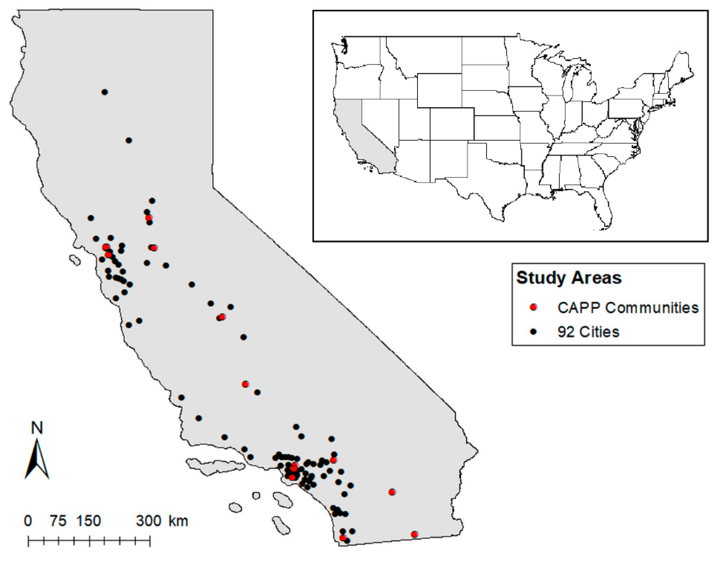
Figure 1 depicts a map with locations of the thirteen communities included in CAPP at the time of this study. Shapefiles for each community were obtained from CARB in 2020 and linked spatially to the high-resolution PM
2.5 dataset based on overlapping 1 km
2 grid centroids. Additionally, the nearest active PM
2.5 monitor was identified for each community, and their 4-year daily averages obtained from the U.S. EPA Air Data for comparison (
https://www.epa.gov/outdoor-air-quality-data, accessed on 2 January 2022). Of the thirteen communities, seven had a monitor inside the community, five had monitors within 5.1 km from community boundaries, and one community (Shafter) had a monitor 21.1 km away. The 24 h Federal Reference Method (FRM) primary monitor data were used from each site, except in cases where only Federal Equivalent Method (FEM) monitoring data were available within a relevant distance to the community. FRM monitors use manual gravimetric methods measuring PM
2.5 mass over 24 h periods, while FEM monitors may be manually operated or automatic as long as they meet strict operating specifications [
32]. FEM sites in this analysis included the Richmond/San Pablo, West Oakland, and Stockton communities, whose monitoring data came from continuous samplers reported as hourly data and aggregated to produce 24 h averages. FRM/FEM methods are well-validated and controlled and are required for air quality data used to inform compliance with national standards. They were selected for use in this study because their data are commonly used in exposure and health impact research, including use as a validation tool for air quality models and low-cost sensors [
11,
16,
17].
Local daily bias of the exposure model was calculated for each community by comparing each community’s ground monitor observations with its nearest model estimates (all estimates within a distance of 1 km from the monitor). For days with a monitor measurement, the daily bias value was calculated and used to adjust all community model values. The four-year (2015–2018) averages of these biases were then calculated for each community, and this daily bias average was used to correct model estimates on days without a monitor measurement. Average differences between ground measurements and MAIAC-derived predictions ranged from −2.24 to 0.66 µg/m
3 among the thirteen communities, which is well within the range of ±3 µg/m
3 estimated from a ten-year analysis of MAIAC estimates in the southeastern U.S. by Hu et al. (2014) [
10].
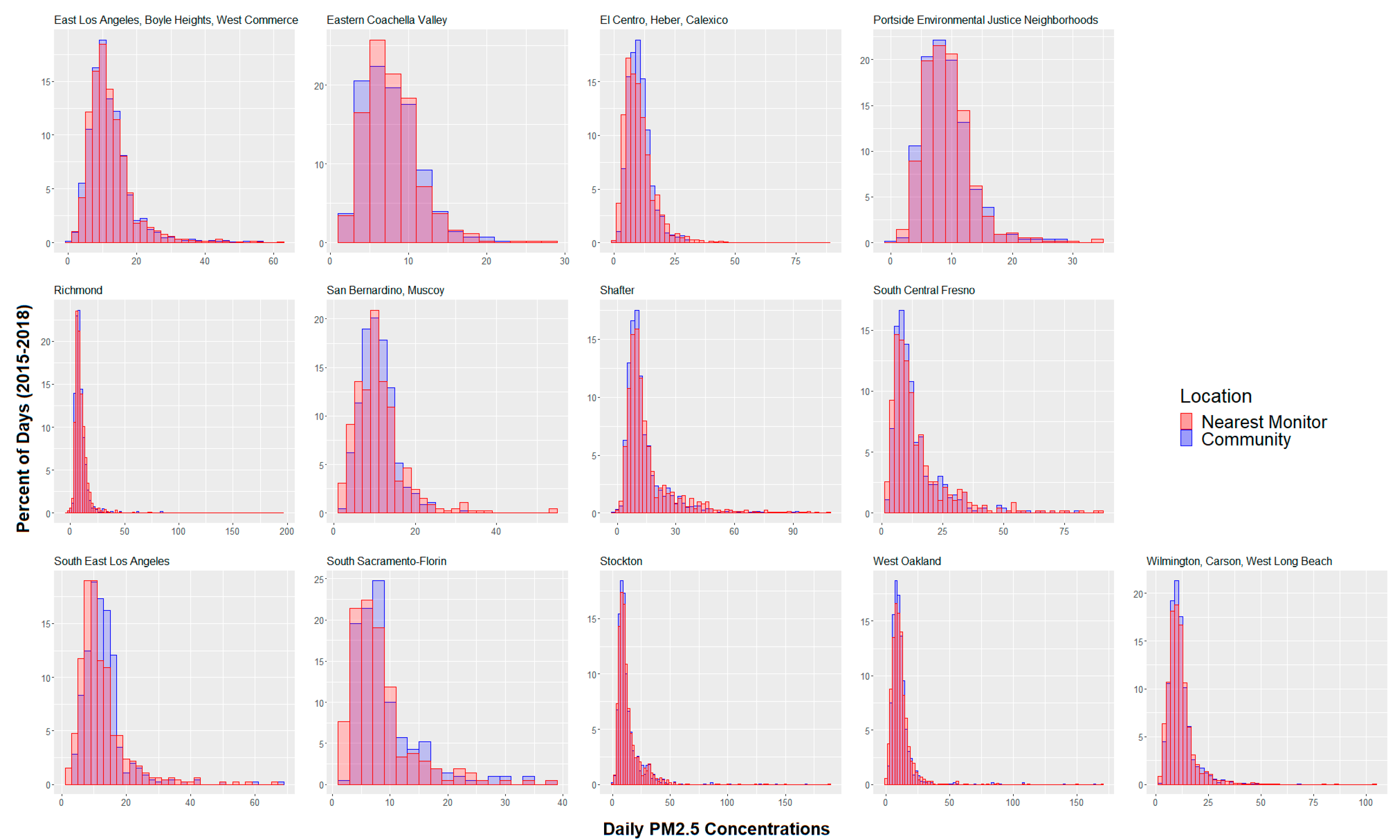
Using these corrected values, separate temporal and spatial analyses were performed for each community. To assess how well ground monitors capture day-to-day changes in community exposures, we created histograms showing the distribution of daily pollution estimates from modeled estimates compared with those from nearest monitor daily measurements. For spatial analyses, we created maps depicting four-year averages for all model estimates and their nearest monitor and examined their concentration gradients for exposure variations.
Additionally, presented in
Figure 1 are the locations of all cities in California with three or more Zone Improvement Plan Codes (ZIP Codes) (
N = 92). For this sample, ZIP Codes were linked spatially to their primary city following the December 2019 United States Postal Service-defined boundaries [
33]. ZIP Codes were then merged with our high-resolution PM
2.5 data based on overlapping 1 km
2 grid centroids (ranging from 1 to 1141 centroids per ZIP Code) and averaged to produce ZIP Code-level daily concentrations.
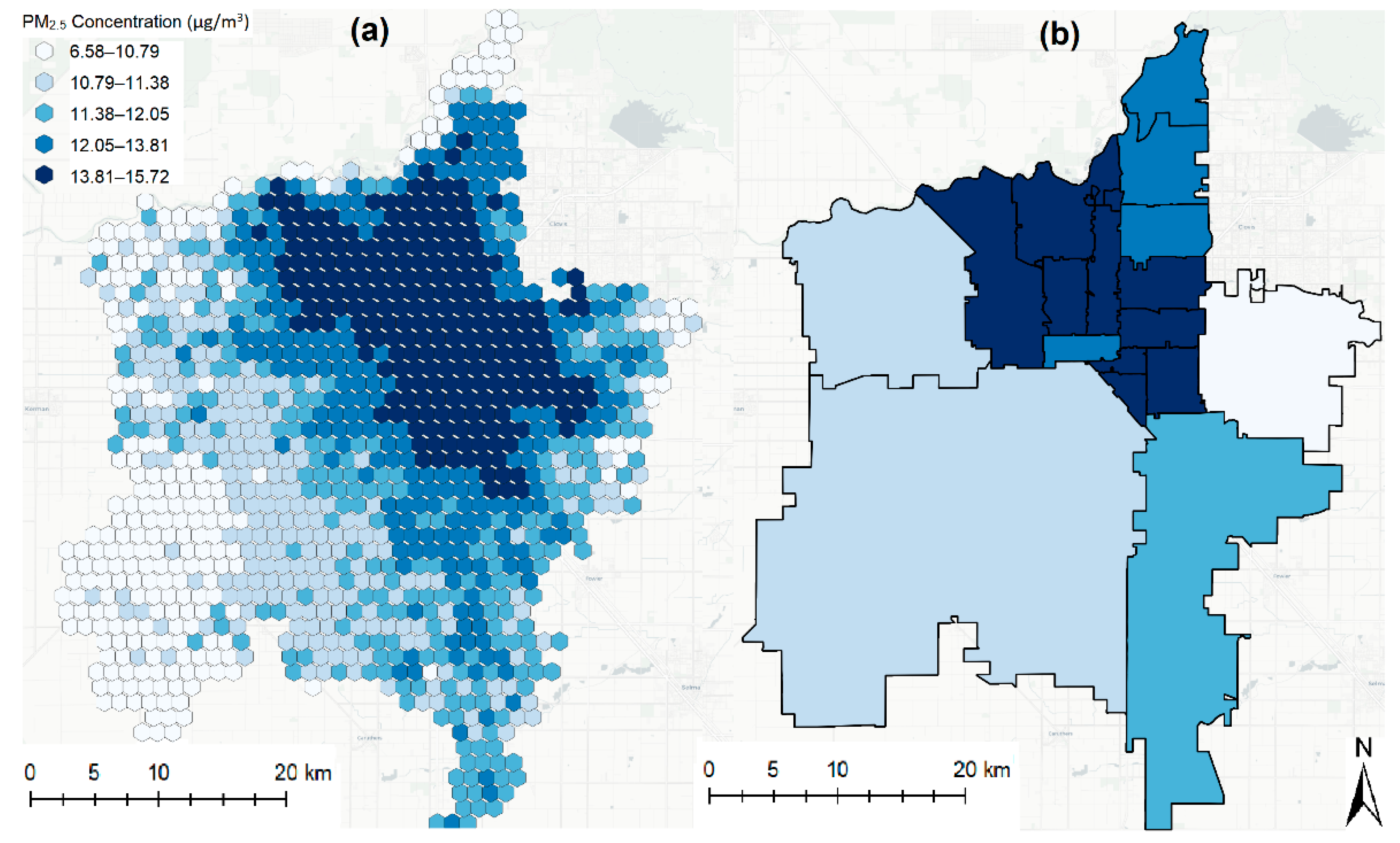
Figure 2 presents a simple visual example of these two spatial resolutions in the city of Fresno.
Daily Coefficients of Variation (CV) were calculated for all ZIP Codes (
N = 590) to compare within-ZIP Code variations. The CV was selected as a measure of ZIP Code-level variation due to its ability to produce relative variances that can be compared among different groups. In this case, the CV represents the relative difference in PM
2.5 concentrations among 1 km
2 resolution estimates within a ZIP Code. Daily CVs were calculated for each ZIP Code using Equation (1), based on methods presented by Dai et al. [
34]:
where
is the PM
2.5 concentration of the ith 1 km
2 resolution estimate,
is the mean PM
2.5 concentration of the ZIP Code, and
n is the number of 1 km
2 resolution estimates in the ZIP Code. In order to examine variation at the 1 km
2 resolution scale, a daily relative percent difference (RPD) was calculated for each 1 km
2 resolution estimate as shown in Equation (2):
Daily PM
2.5 concentrations and variance statistics (CV and RPD) were aggregated by region, season, and ZIP Code area. Northern and Southern California were defined as cities north and south of the 36th parallel north, respectively. In order to account for the effects of seasonal ozone changes, our warm season was defined according to which half of the year had the highest ozone levels on average during the four study years in our study areas based on daily 8 h max data provided by EPA Air Data (
https://www.epa.gov/outdoor-air-quality-data, accessed on 2 January 2022); this resulted in a warm season from April–September and a cold season from October–March.
Finally, subsequent models were created in order to compare potential exposure bias and misclassification in the study sample. The first model was designed to assess exposure biases due to differences in spatial resolution. For the study’s largest-population city (Los Angeles), 100 random coordinates were sampled to represent “home” locations, and their 1 km2 and ZIP Code resolution estimates were plotted against one another for each of twenty dates randomly sampled from the study period. A second model was then created to examine exposure misclassification due to the assumption of daily exposures based solely on home address locations. Here, 100 additional city coordinates were randomly sampled as “work” locations and paired with the initial home locations. Because the intent of this analysis is to create a simple example comparing the impacts of diurnal movement vs. spatial resolution on exposure misclassification, the labels “work” and “home” are only intended to differentiate the two locations and do not represent true commercial and residential areas. Assuming each pair represented an individual who spends 50% of their time at home and 50% of their time at work (again, this is an illustrative value not intended to reflect true temporal patterns), the daily 1 km2 resolution estimates for each location was calculated. These were then plotted against the 1 km2 resolution estimates of the home-only model using the same randomly sampled dates from the first model. R-squared values were calculated for all correlation plots, then averaged across both models and compared.
All analyses were run using R version 4.1.0 [
35] and ArcMap version 10.8.1 [
36].
3. Results
A summary of the CAPP communities is presented in
Table 1, with areas ranging from 17 to 747 km
2. Most communities had a monitor less than 1 km away, with a maximum distance of 21 km to the nearest site (Shafter). After correcting community estimates for model bias, the four-year PM
2.5 daily averages were well represented by nearest monitor measurements, with most community averages falling within 1 µg/m
3 of their nearest monitor. No obvious relationship between monitor distance or community size is apparent from these summary statistics.
Temporal differences between ground observations and modeled estimates are presented in
Figure 3. Here, histograms comparing the frequency of daily PM
2.5 concentrations for modeled community averages versus ground monitors reveal a strong temporal correlation between the two exposure assessment methods for all thirteen communities. A slight underestimation of daily community values occurs in Southeast Los Angeles and South Sacramento—Florin, whose distributions for monitored data have modes about 2 µg/m
3 lower than the modes of modeled values. These two communities have moderately distanced monitors (3.9 and 5.1 km away, respectively); however, no underestimation is observed in Shafter, whose monitor is over 20 km away.
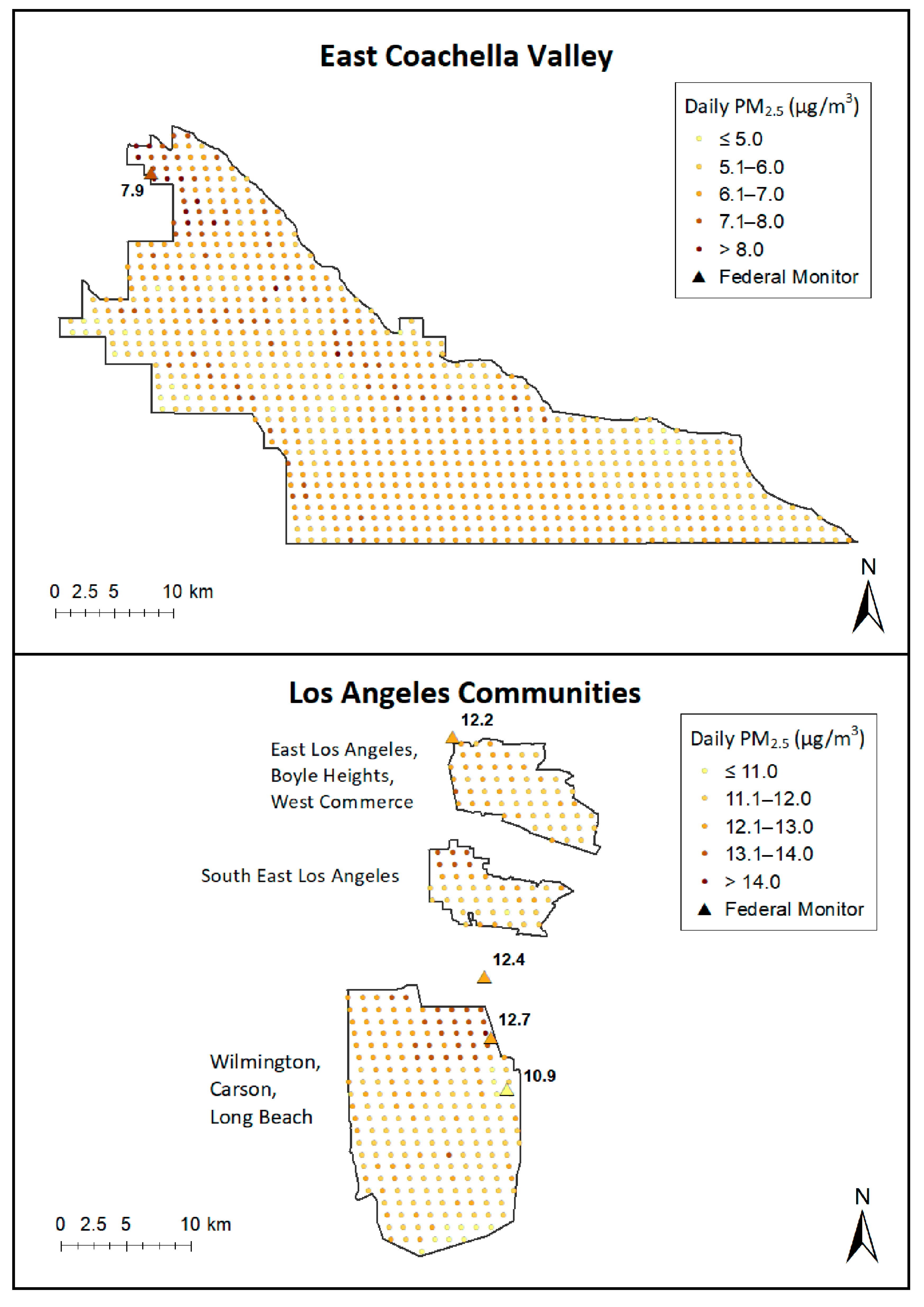
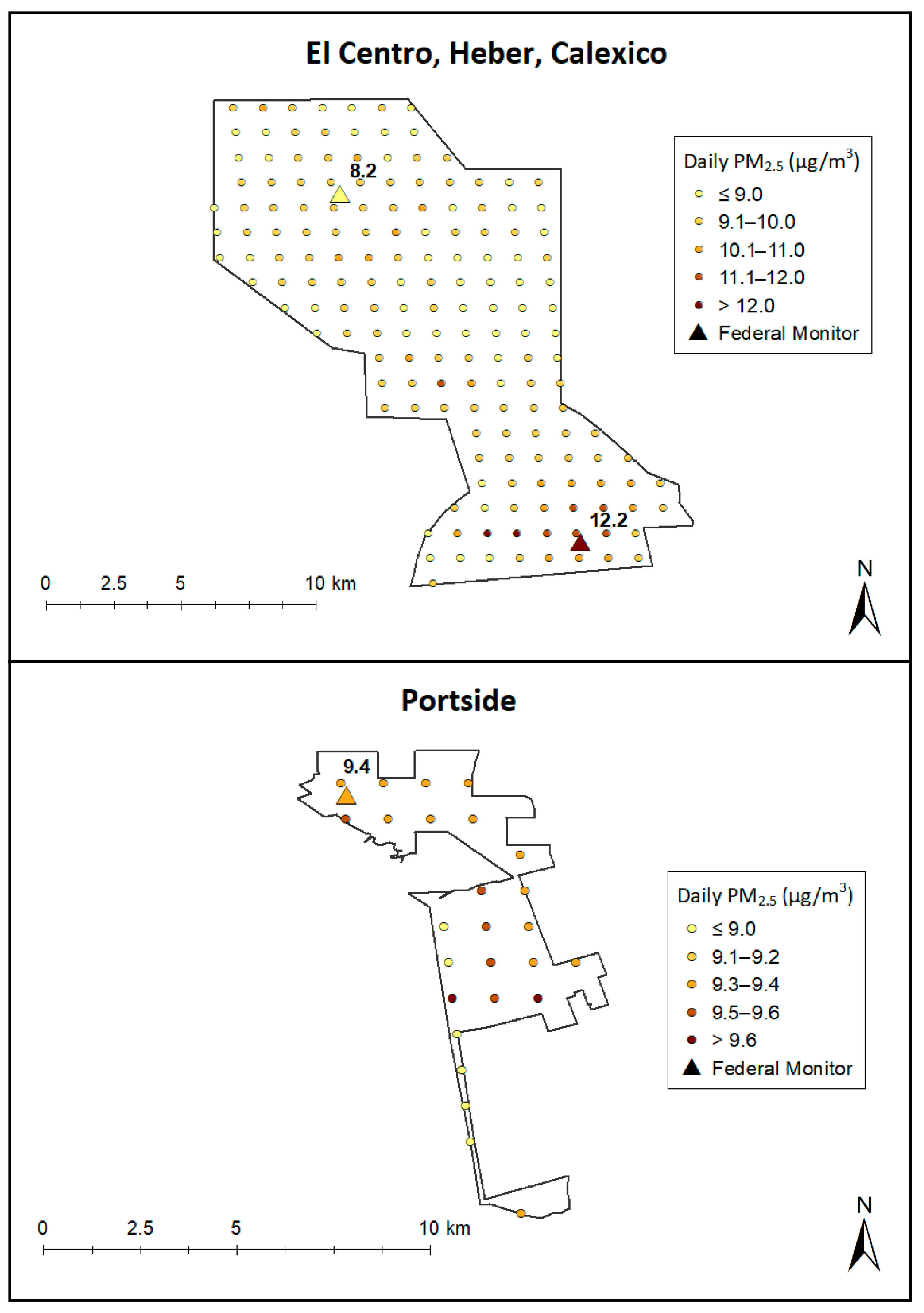
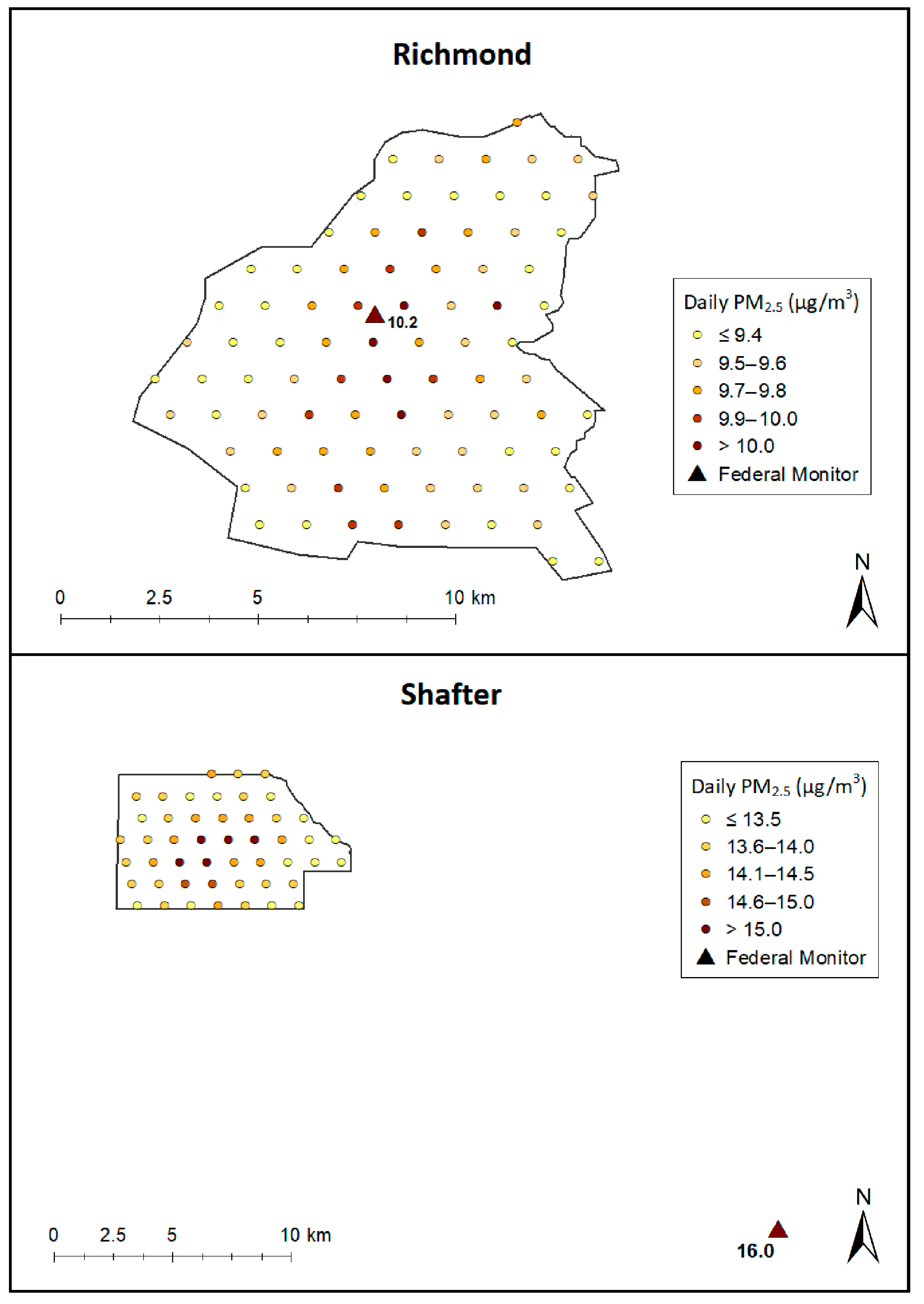
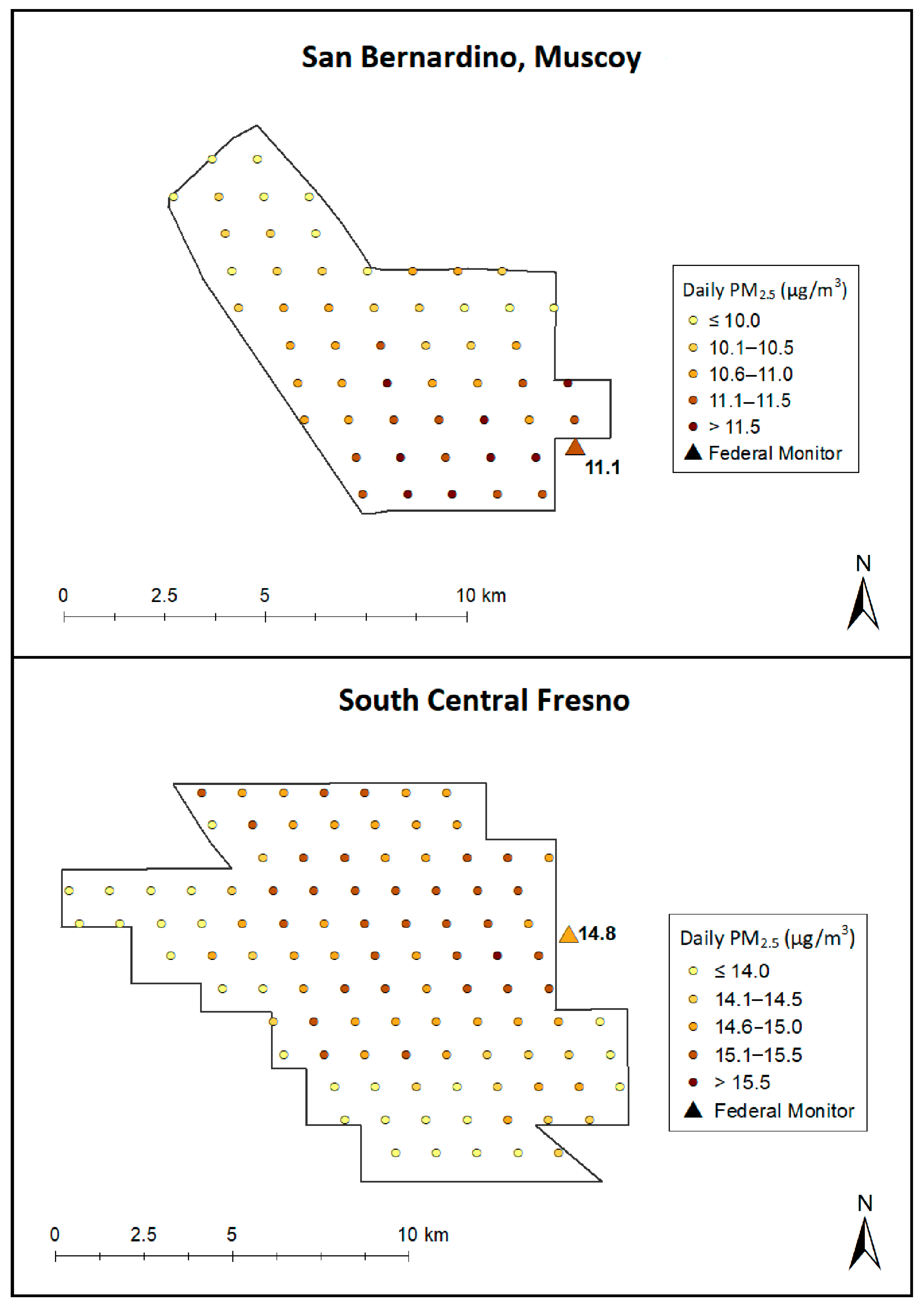
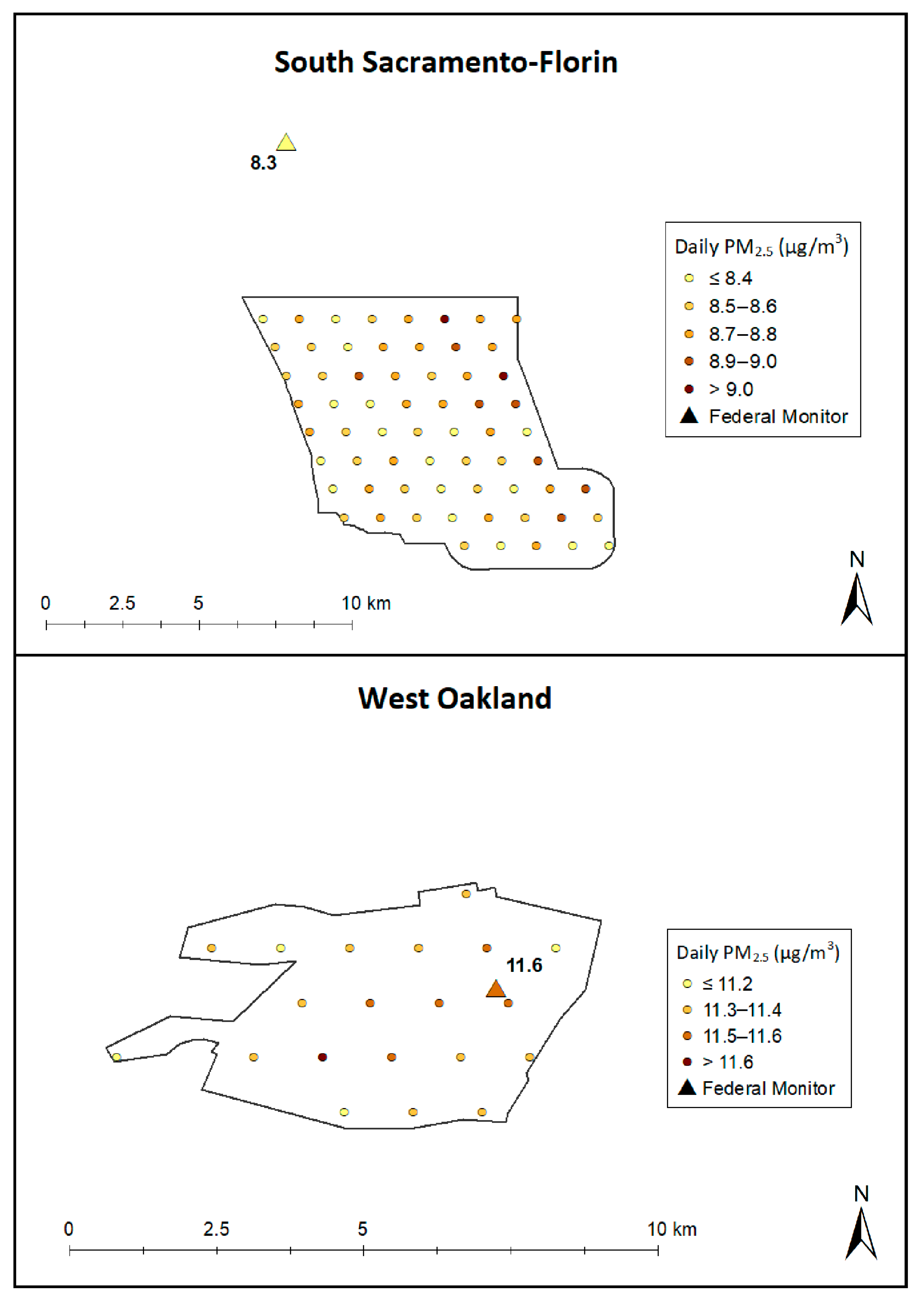
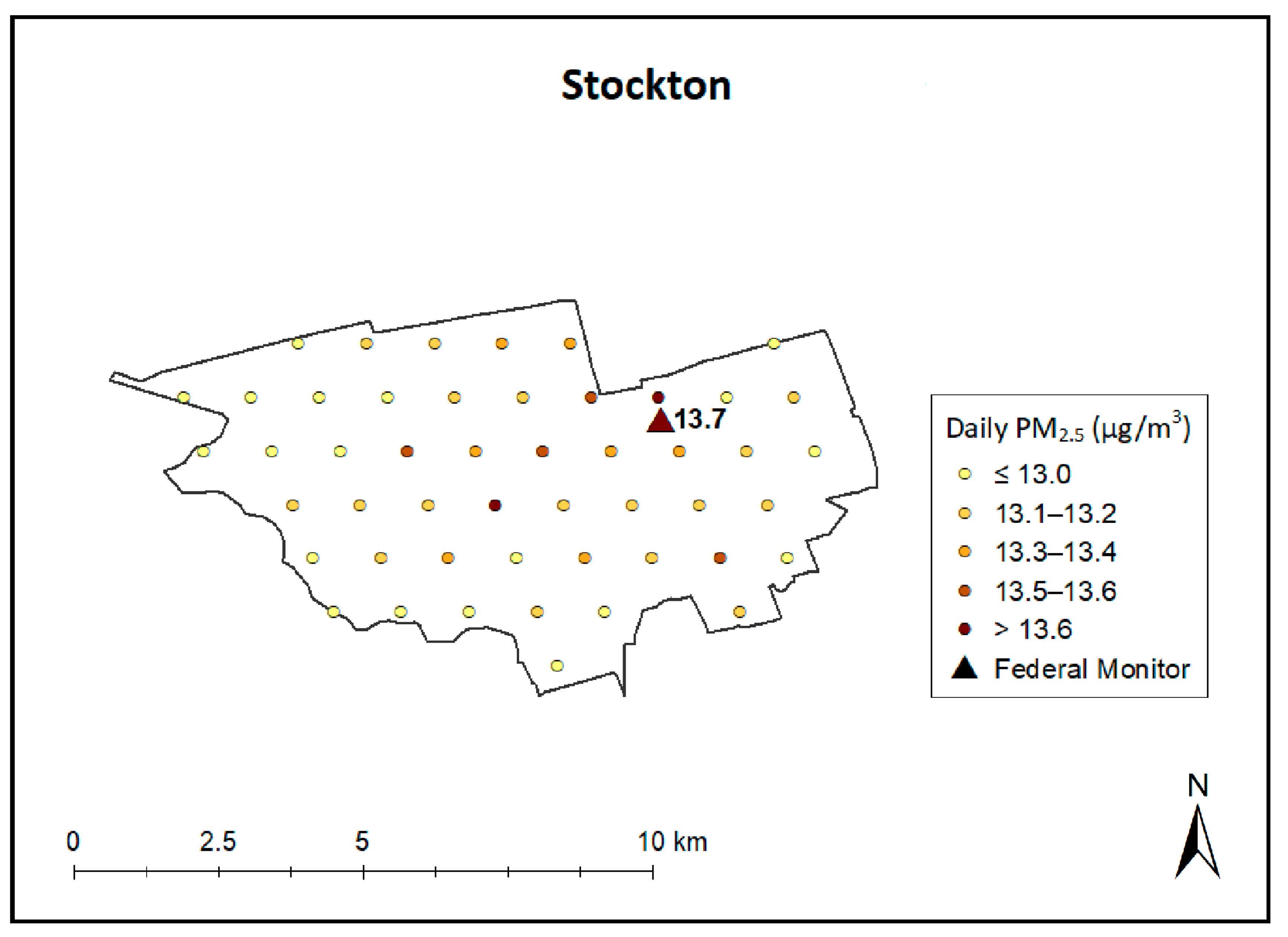
In contrast, maps of 4-year average daily PM
2.5 reveal spatial gradients of varying scales across all thirteen communities (
Figure 4). Among communities with both strong (the three Los Angeles communities, South Sacramento—Florin) and weak gradients (East Coachella Valley, San Bernardino—Muscoy, South Central Fresno, West Oakland), we found spatial differences in exposure within the community that their nearest ground monitors cannot capture. Even though many of these ground measurements provide a fair representation of their community’s average exposure, they mask variations, resulting in an incomplete exposure profile. Other communities in our sample have monitors located at the highest pollution sites, including Portside, Richmond, and Stockton. While these measurements provide more complete exposure profiles, there remain additional polluted areas within each of these communities whose location details are unavailable without more highly resolved data. Additionally, these central site monitors provide little to no information regarding the extent and boundaries of concentration gradients.
Table 2 summarizes the PM
2.5 concentrations and variances for all ZIP Codes across the study sample, with subsets by ZIP Code area. Here, geographic area is approximated using the number of 1 km
2 centroids within its boundaries, i.e., a ZIP Code with 10 estimates will have an area of 10 km
2. CV values represent relative within-ZIP Code variances that can be compared and aggregated across the state. The CV is presented as a percentage ranging from 0 to 100; a higher CV indicates greater variance among the 1 km
2 resolution estimates within a ZIP Code, while a lower CV indicates less variance within a ZIP Code. In this sample, the year-round CV was 7%, indicating relatively little variance within ZIP-codes. This trend was consistent across regions and seasons, with slightly higher CV values during the cold season (CV = 9%) and the lowest in the warm season (CV = 6%). Looking at these results by ZIP Code area, within-ZIP Code variation increases with increasing ZIP Code size, reaching 14% year-round and statewide for ZIP Codes with areas larger than 50 km
2. Additionally, within-ZIP Code variations increase during the cold season, the highest being observed in the largest ZIP Codes in Southern California (CV = 21%). Generally, these increases in CV are negligible in smaller ZIP Codes (less than 50 km
2).
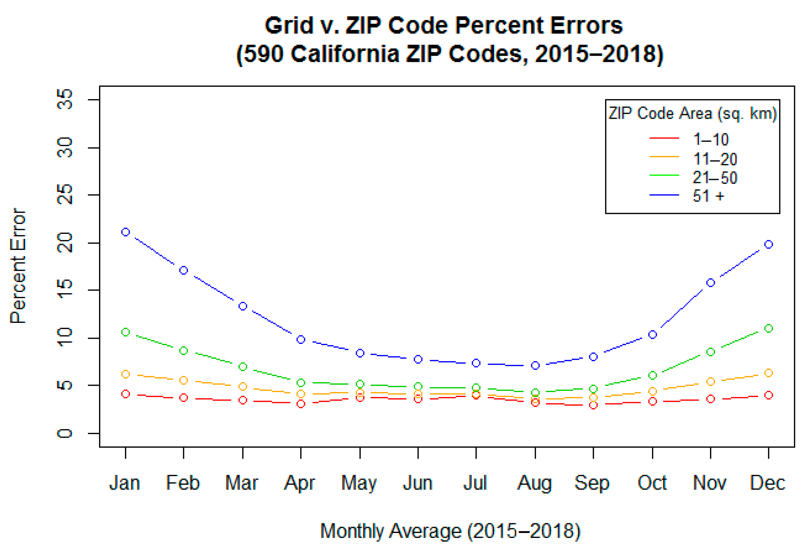
Figure 5 presents four-year monthly averages of RPDs between 1 km
2 resolution estimates and their corresponding ZIP Code average, grouped by ZIP Code area. This plot reveals little difference between RPDs among the smallest ZIP Code groups (with areas up to 50 km
2) during the warm season, while RPD increases incrementally with ZIP Code area during the cold season among all groups. For ZIP Codes larger than 50 km
2, RPDs are greater than smaller ZIP Codes year-round and average over 20% during the coldest months.
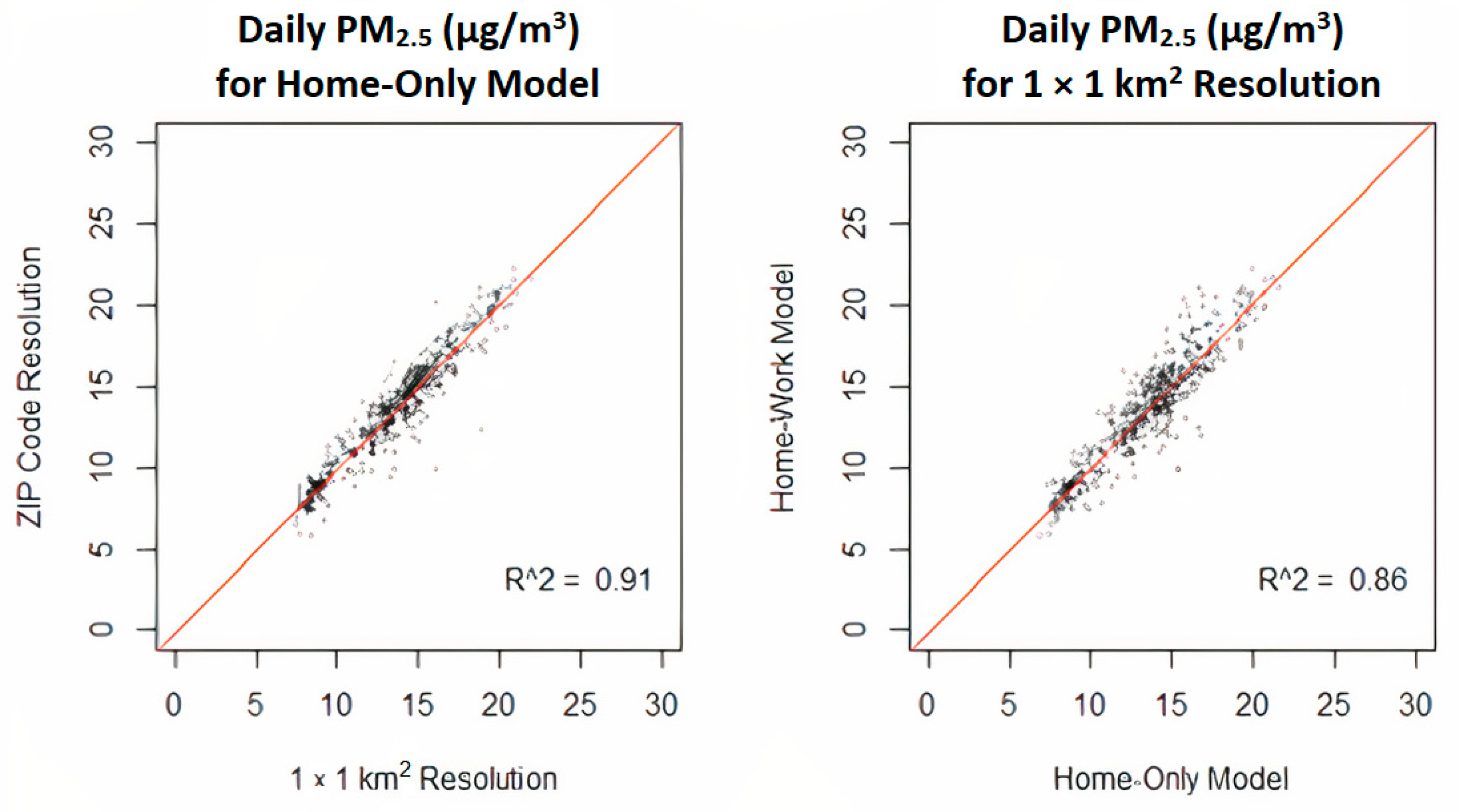
Finally, the Los Angeles correlation plots resulted in slightly better fits when comparing differing spatial resolutions versus differences in home-only and home-work modeled concentration estimates. For the twenty dates randomly selected between 2015–2018, correlation plots comparing 1 km
2 and ZIP Code-level resolutions for the home-only model had an average R
2 of 0.95 (ranging from 0.89–0.98), while those comparing 1 km
2 resolution estimates of the home-only to the home-work model had an average R
2 of 0.92 (ranging from 0.85–0.96).
Figure 6 presents an example for one of these paired comparisons.
4. Discussion
In this study, we compared ground monitors to an integrated dataset of high-resolution, uniform PM2.5 estimates in their respective ability to capture critical spatiotemporal patterns of air pollution in high-risk communities. We found that among California communities most impacted by environmental injustice (namely, those with disproportionate pollution exposures), regulatory ground monitors are generally successful in capturing the day-to-day changes in PM2.5 but are less effective at capturing spatial variations in neighborhood exposures. While the exposure profiles of these disadvantaged neighborhoods become much clearer using satellite-derived pollution estimates, we found that ultra-high-resolution data at resolutions of 1 km2 offer little additional information to the average California community as compared to estimates made at the ZIP-code level. This information is vital when designing effective strategies to reduce the emissions of PM2.5 and its precursor gases and the health impacts of air pollution among communities at the highest risk of air pollution health impacts.
Gaps in ambient air quality monitoring data are not homogenous. Sullivan and Krupnick (2018) found that 24.4 million people in the U.S. live in counties exceeding PM
2.5 NAAQS based on satellite assessments yet federally classified as in attainment [
37]. For reference, U.S. national PM
2.5 standards are set at 12 µg/m
2 for long-term exposures (based on the 3-year average of the annual mean concentration) and 35 µg/m
2 for short-term exposures (based on the 3-year average of the 24 h 98th percentile concentration) (
https://www.epa.gov/criteria-air-pollutants/naaqs-table, accessed on 2 January 2022). Additionally, recent evidence suggests that the siting of new ground monitors may be impacted by income- and race-based discrimination. Grainger and Schreiber (2019) found that in the U.S., new ground monitors are less likely to be sited in low-income communities and that counties in attainment of EPA standards (with little federal oversight) are less likely to monitor high-pollution neighborhoods unless those areas are largely high-income and white [
38]. Fortunately, this is not the case in California state, as demonstrated by Lee [
39], who found that ground monitors are significantly more likely to be located in communities with larger proportions of people of color, living in poverty, and with lower education levels. Even so, we still observed variations of exposure among CAPP communities that cannot be captured by ground networks alone. Thus, the uniform air quality predictions derived from satellite instruments and modeling methods are vital not only for the unbiased identification of the most high-risk communities for environmental injustice but for improving the spatial resolution of those already identified.
High-resolution pollution estimates are key to characterizing exposures in disproportionately impacted communities, but it is important to understand the resolution needed to detect meaningful differences in pollution exposures. This is an important consideration for local jurisdictions who have limited resources for air quality monitoring and management. In most cases, the variation between ZIP Codes far outweighed the variation within, with the exception of ZIP Codes larger than 50 km2 in area. The latter had relative percent differences among their high-resolution predictions that were consistently higher year-round (and over 10% higher during the winter) than those observed in all the smaller ZIP Code groups. This suggests that regions with any demographic profile where a single ground monitor represents areas larger than 50 km2 would also benefit from high-resolution air quality data and/or expanded ground-level monitoring. Otherwise, for the average community there is little additional information to be gained at resolutions below 50 km2. This is supported by observations of the six CAPP communities with areas larger than 50 km2, with missing information presenting in at least two ways. The large areas of Wilmington, Carson, West Long Beach; South Central Fresno; and South Sacramento–Florin resulted in numerous community concentration variations not being captured by ground monitor measurements. Other large CAPP communities (Eastern Coachella Valley; El Centro, Heber, Calexico; and Richmond) had monitors whose measures successfully captured spatial differences in exposure but could not provide information on their highly variable gradation patterns. In contrast, smaller CAPP communities had fewer changes in pollution at a spatial level and thus had profiles better represented by the nearest monitor.
This idea of diminishing returns from very high-resolution spatial air quality data is supported in the existing literature. In a comparable analysis, Lee [
39] examined variations in exposure among 55 urban areas in California using 1 × 1 km
2 resolution PM
2.5 estimates derived from MODIS MAIAC AOD. Within-urban PM
2.5 variability was between 31.4–35.6% of the between-urban variability throughout the state (although this percentage was notably larger in more highly populated areas). A study by Dai et al. [
36] in China, whose methods served as a model for our work, supports the dominance of temporal over spatial variance in PM
2.5 urban exposure assessment. Their study compared between- and within-urban variation of PM
2.5 from monitoring stations in five Chinese megacities, finding greater concentration differences between cities than within. This was very similar to our observations from 92 California cities, wherein between-ZIP Code variance was predominant. Furthermore, in all five cities in the Dai et al. study greater variations were observed by season than by distance from city center (see Figure 10 of the study). Similarly, our analysis found much more profound changes in PM
2.5 concentrations throughout the year than between 1 km
2 and ZIP Code-level estimates on any given day. Specifically, in
Figure 5 we see how the differences in RPD between different ZIP Code areas become more pronounced during the colder months; during the warmer months, the RPDs among the three ZIP Code groups with areas below 50 km
2 are barely distinguishable. Though at different geospatial scales, both studies confirm that improvements in intra-urban spatial resolutions for PM
2.5 result in smaller gains in exposure information relative to greater temporal-level data. This concept is further supported in a study by Huang et al. [
40], which used satellite-derived estimates coupled with road-level monitors to produce spatiotemporal prediction models for PM
2.5 concentrations in New York City at 100 m resolutions for 2015. Rankings of variable importance in their random forest models clearly indicate that temporal predictors dominate over spatial ones (see
Figure 3 of the study). While it is true that the spatial variation of PM
2.5 within the city is apparent (see
Figure 5 of the study), the lowest concentration category on these maps is approximately 7.0 µg/m
3, implying that the spatial model has a large intercept and further supporting the greater impact of temporal variables in these models. Likewise, our analysis of 92 cities produced relatively narrow concentration ranges day-to-day compared to monthly and seasonal variation. Thus, when both spatial and temporal data are available for daily PM
2.5, its temporal variation is likely to overwhelm spatial variation.
The similarities of PM
2.5 estimates at either 1 km
2 and ZIP Code-level spatial resolutions are fully consistent with this pollutant’s dispersion patterns. Commonly formed as a secondary pollutant, PM
2.5 emerges after its precursor gases have undergone a significant number of chemical reactions throughout an urban area [
41]. In contrast, primary pollutants arising from traffic pollution, including nitrogen dioxide (NO
2) and carbon monoxide (CO), show highly heterogeneous distribution patterns within cities that typically align with major roadways. These differences have implications for environmental justice, as supported in a study by Rosofsky et al. (2018), where inequalities in exposure levels were larger for NO
2 than PM
2.5 between different sociodemographic groups [
42]. Additionally, different PM fractions may themselves vary in dispersion patterns. Coarse PM mass tends to deposit closer to its source due to gravitational settling, while ultrafine particles show strong gradients near heavy traffic sources due to their short half-lives before coagulating into larger particles [
43,
44]. Thus, had the present analysis been performed using a pollutant with known heterogeneous intra-urban dispersion patterns, the variance within ZIP Codes would likely have been greater than what was observed with PM
2.5.
This assumption is supported by previous studies comparing the variations of intra-urban resolutions between PM
2.5 to other traffic-related air pollutants. Using a spatial decomposition approach to breakdown major air pollutants by major source, a nationwide analysis by Wang et al. [
45] found that local PM
2.5 is composed mainly from regional sources, with little variability within cities and no clear spatial gradients at resolutions smaller than 1 km. In contrast, NO
2 showed significant differences in mean concentrations at intra-urban spatial levels, as it is derived primarily from neighborhood-level traffic sources. This work suggests that the geographical level at which a pollutant is derived is also the level where the greatest variability in its concentration is observed. Because of the strong contribution from regional industrial emissions to PM
2.5 concentrations, highly refined intra-city spatial resolutions are unlikely to provide more information than larger resolutions, a conclusion supported by our results in California urban areas. Additionally, Wang et al. observed slight increases in the variability of PM
2.5 for larger urban areas; similarly, we found increases in within-ZIP Code variability for ZIP Codes with areas larger than 50 km
2.
Compared to limited spatial resolutions, greater information gaps may be due to exposure misclassification from the lack of individual movement-based data for those commuting to different areas within their city throughout the day. This was true in our sub-analysis of Los Angeles, which found a higher correlation between 1 km
2 and ZIP Code-level resolutions than between models that did and did not assume a home-only location. In other words, missing location data on individual movement patterns may be a larger source of exposure misclassification than the bias created from lower spatial resolutions. This relatively simplistic model is supported by a more complex analysis of Los Angeles residents performed by Lu (2021), in which personal PM
2.5 exposures (using 500 m
2 gridded model estimates) were underestimated by 22% for all workers and up to 61% for those with the longest commutes when mobility data were excluded from the model [
46]. By incorporating more highly resolved location-based data, a wealth of new information can be obtained pertaining to environmental justice. In the case of Lu (2021), mobility data narrowed exposure gaps between White vs. ethnic minority and low- vs. high-income groups by including the higher-level exposures from work and other activities outside the home [
46]. Similarly, Park and Kwan (2020) found that daytime exposures were more equal among racial groups given similar daytime urban pollution exposures, and that home-only models may underestimate total daily exposures for White populations [
47]. Clearly, we still have much to learn regarding environmental disparities in the context of urban air quality. Without near-real time location information on a population, higher spatial resolution data (i.e., less than or equal to 1 km
2) cannot be used to assess local exposures in any meaningful way. As part of their call for integrated exposure science methods, authors of the 2017 ATS Workshop Report [
11] suggest incorporating information already available from other sources, such as social metadata on time-activity patterns, which can significantly increase the spatiotemporal resolution of health studies. Shifting the research focus of PM
2.5 exposure assessment from spatial resolution improvements to better activity-level estimates may ultimately provide richer information for calculating urban air quality impacts on health.
Ultimately, our comparisons of intra-urban spatial resolutions in cities across California suggest that for the average community, little health-relevant information is lost by aggregating 1 km
2 resolution estimates to ZIP Code levels, except for ZIP Codes larger than 50 km
2. However, we acknowledge that these diminishing returns may be largely due to the current limitations in the modeling of remote sensing data. When looking solely at PM
2.5 estimates from MAIAC MODIS AOD and similar products, there are decreasing marginal improvements in their ability to define the spatial variation observed within an airshed due to a limited number of surface reference monitors [
12]. Future work could better assess the full magnitude of this limitation by combining remote sensing products with additional inputs, such as local traffic, weather, and emissions source data. Additionally, similar work could compare or incorporate results from different exposure assessment methods, such as low-cost sensors. Much like satellite-based data, low-cost sensors can help circumvent the limited spatiotemporal resolution of federal ground monitors. This was demonstrated in a study by Danek and Zareba (2021) in Krakow, Poland, where public data from a dense low-cost sensor network successfully differentiated particulate matter (PM) produced by solid fuel heating from transportation and other background sources, as well as identifying the neighboring municipalities contributing most to increased PM diffusion [
48]. In this case, the increased spatiotemporal resolution offered by this low-cost network provided highly useful information, which government networks could not capture.
New environmental justice communities will be added to CAPP as this program expands in future years. With this comes the opportunity to improve the existing selection process and its associated screening tools so that those areas which would benefit most from higher resolution community monitoring can be correctly identified. At present, the CalEnviroScreen mapping tool drives the CAPP community selection process, providing scores for communities based on pollution burdens, health indices, and socioeconomic data (see
https://ww2.arb.ca.gov/capp-selection, accessed on 2 January 2022 and
https://oehha.ca.gov/calenviroscreen, accessed on 2 January 2022). As future versions of this tool incorporate more highly resolved pollution data and additional health and socioeconomic variables, it may also be beneficial to consider new discoveries of the spatiotemporal patterns of criteria pollutants. Using the findings of our study, this might include a priority for 1) communities with sharp spatial gradients of air pollution levels and 2) areas larger than 50 km
2 with only one monitoring site.


 ,
, 


