
Variations in the Peczely Macro-Synoptic Types (1881–2020) with Attention to Weather Extremes in the Pannonian Basin


Abstract
:1. Introduction
- the classification of weather maps into pre-defined discrete types of circulation;
- the impact of global warming on large-scale circulation.
2. Materials and Methods
3. Results
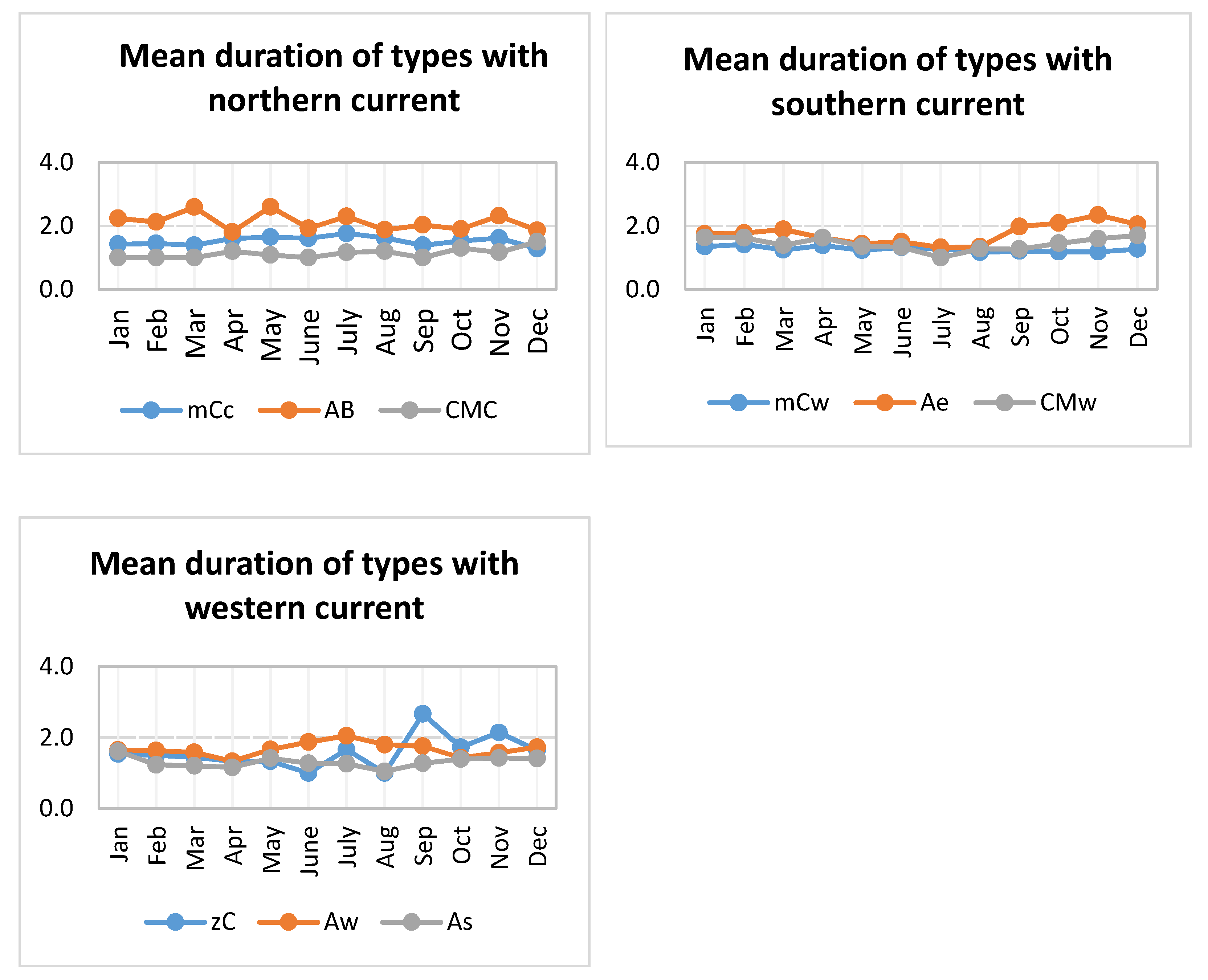
3.1. Monthly Mean Frequency and Duration of the Circulation Types
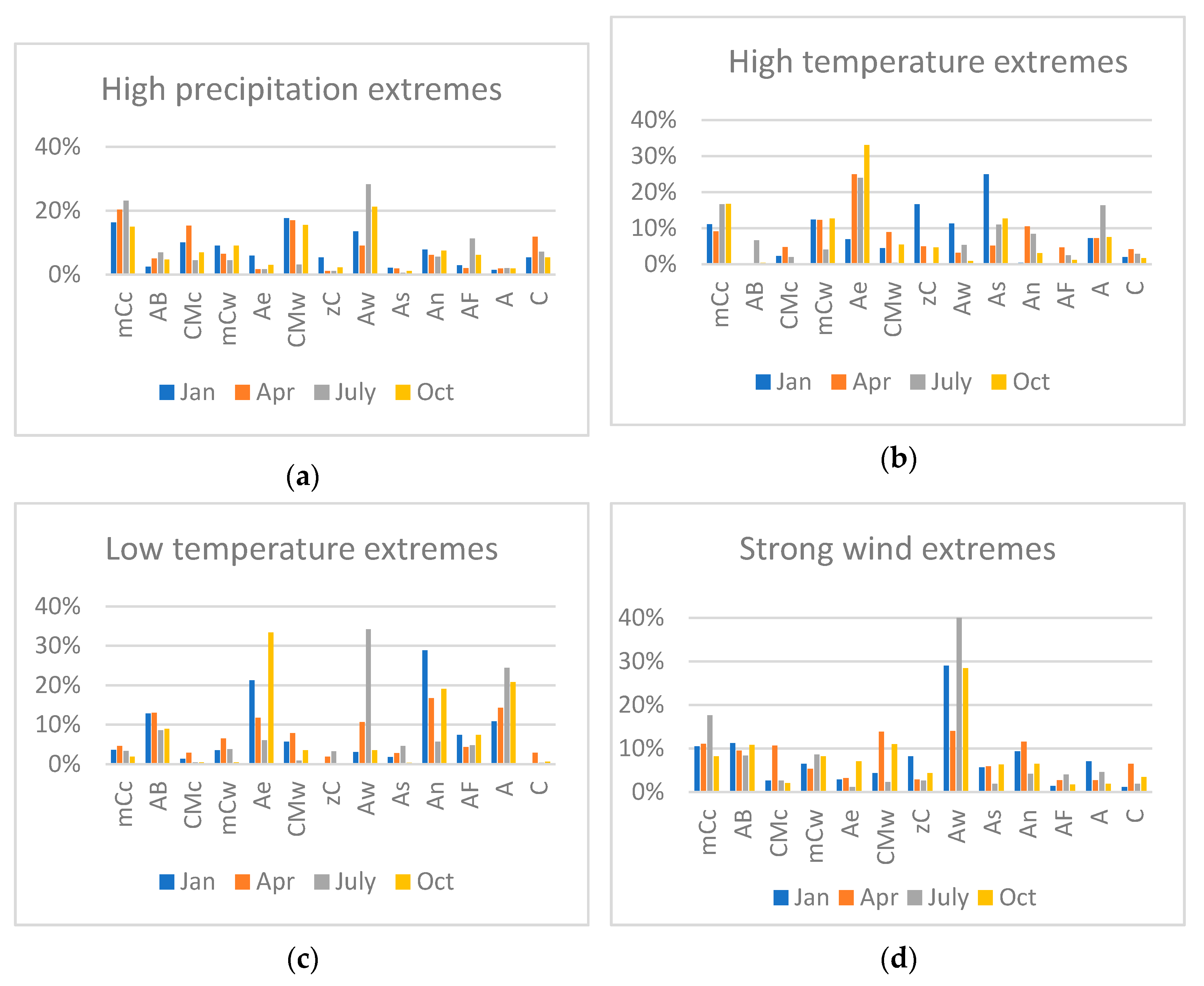
3.2. Distribution of Weather Extremes among the Circulation Types
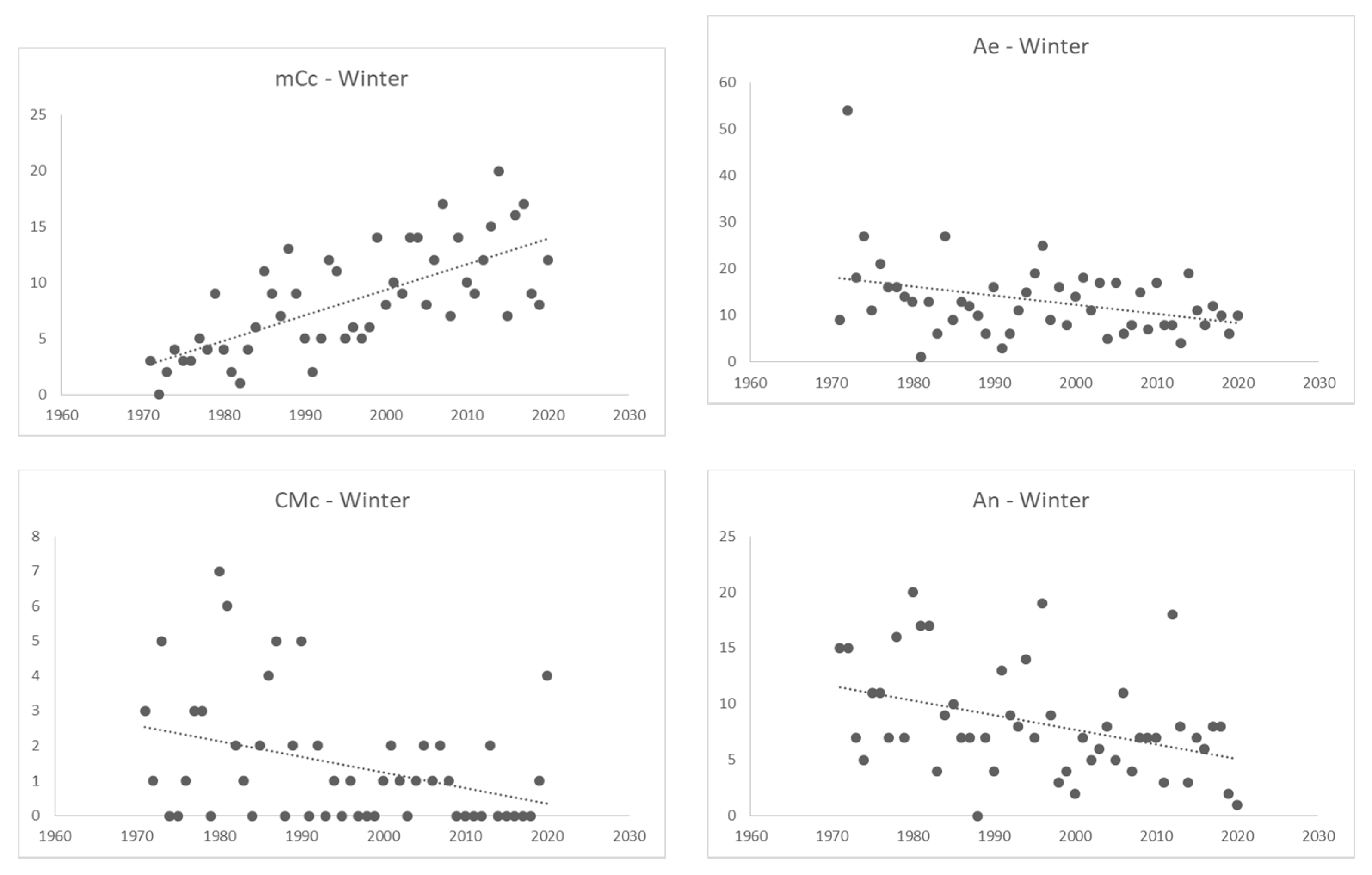
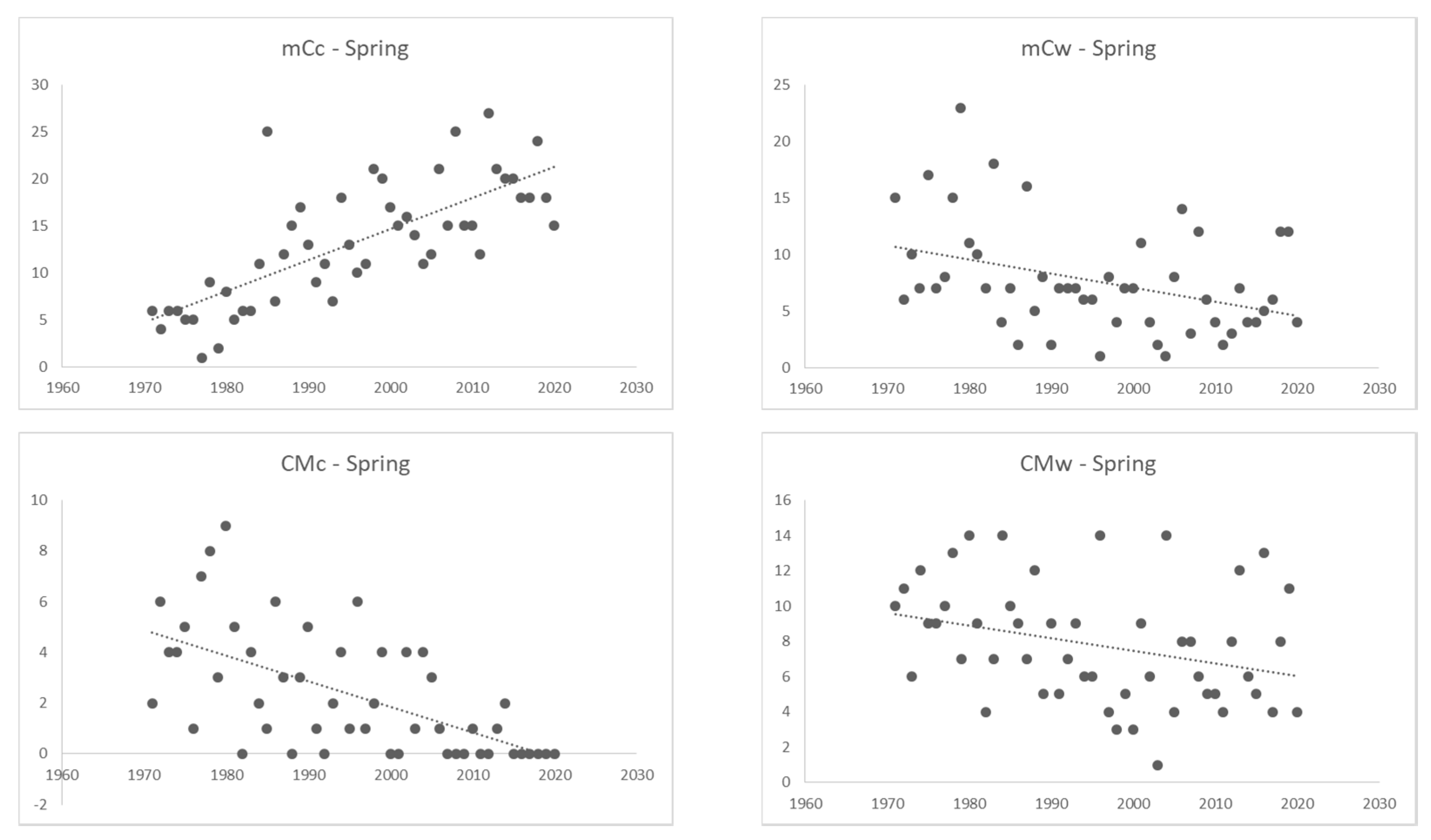
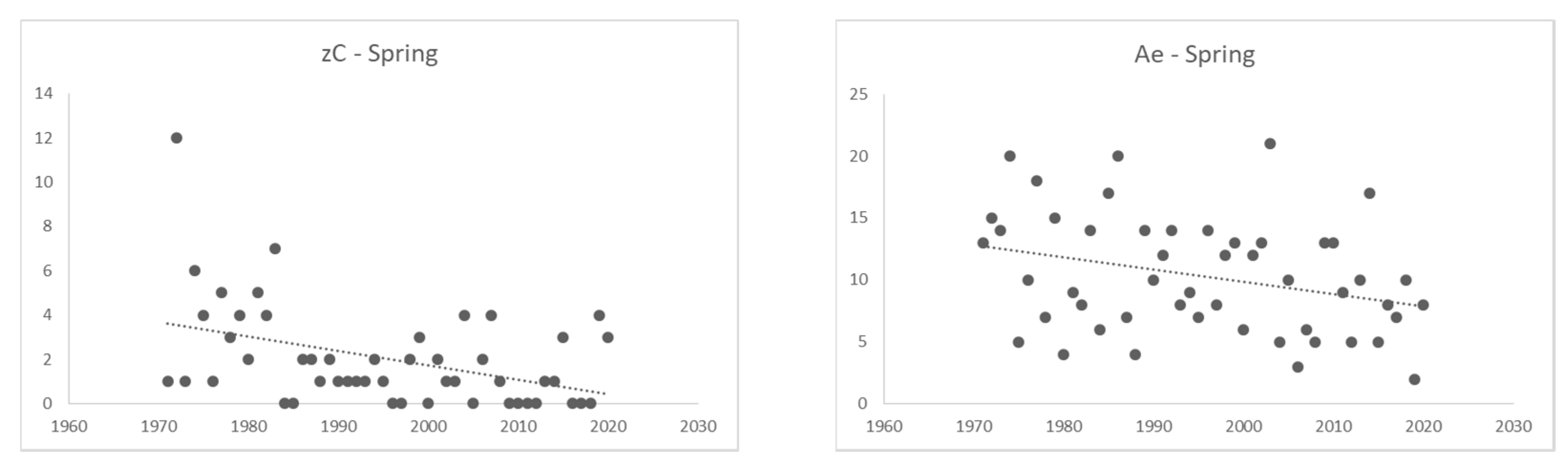
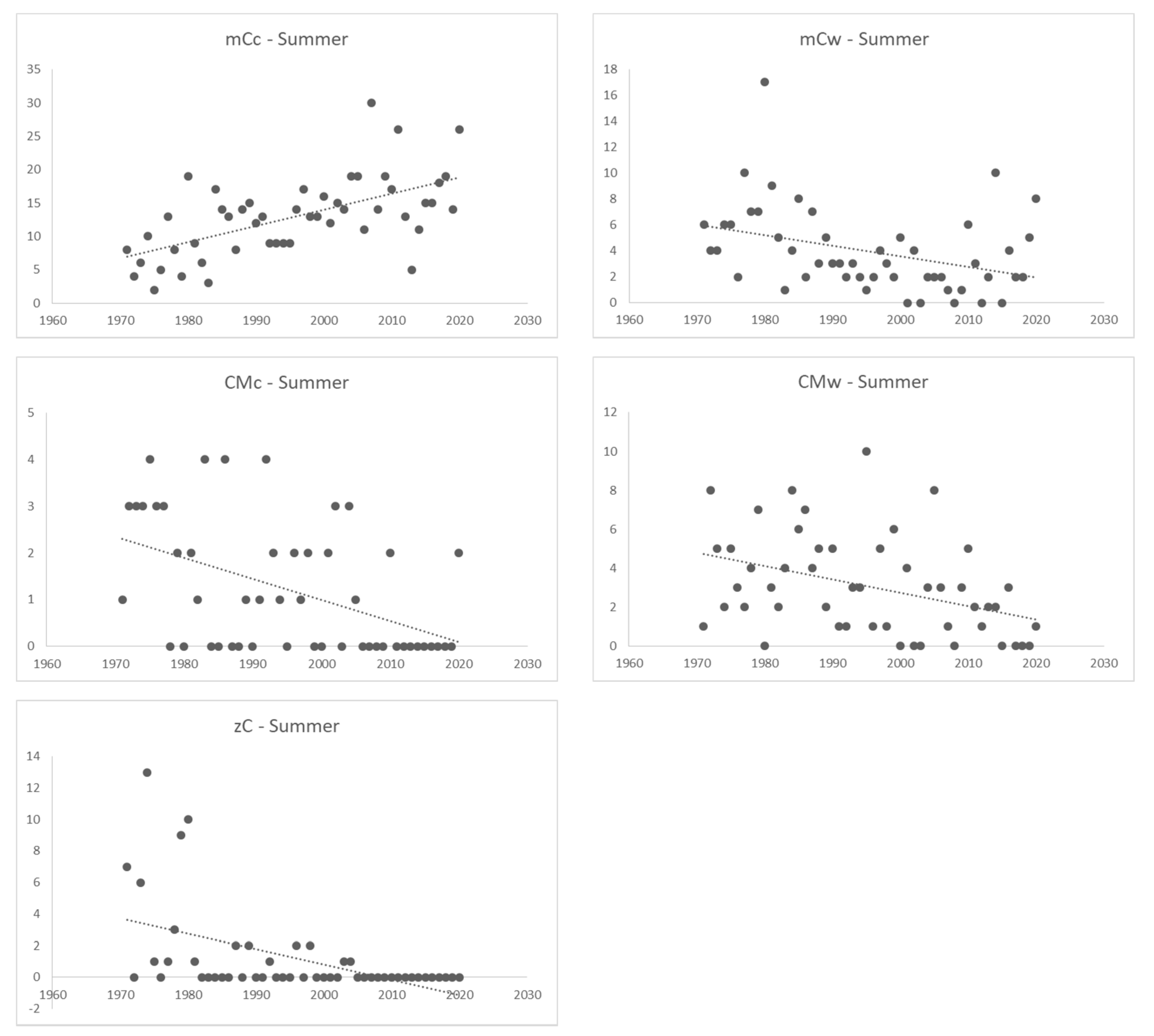
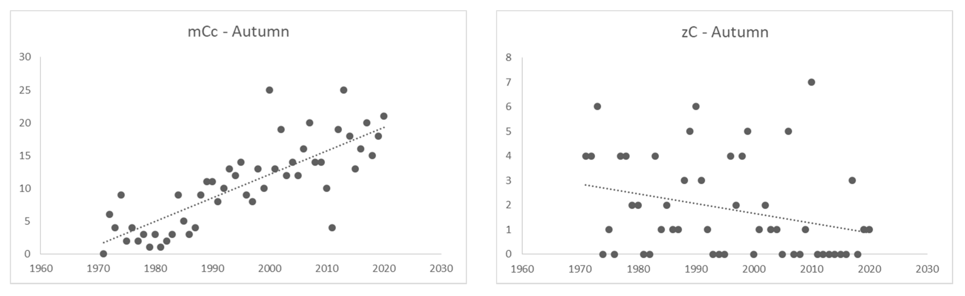
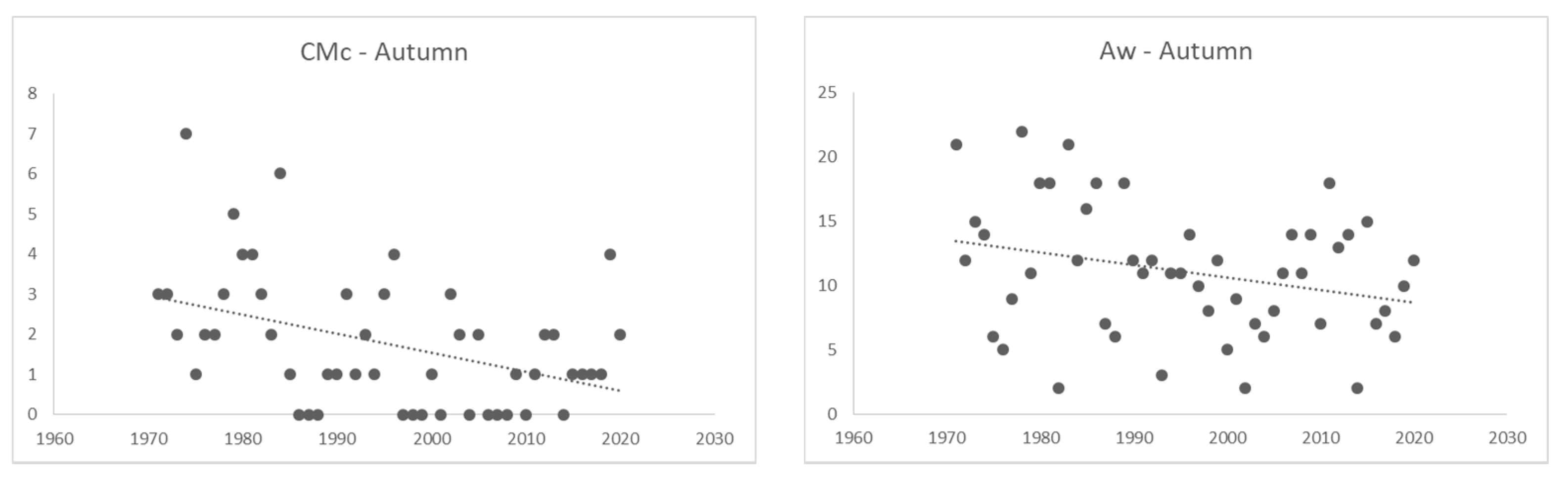
3.3. Trends in Monotonous Hemispherical Warming and Cooling Periods
4. Discussion
5. Conclusions
Author Contributions
Funding
Institutional Review Board Statement
Informed Consent Statement
Data Availability Statement
Conflicts of Interest
References
- Peczely, G. Grosswetterlagen in Ungarn. Kleinere Veröffentlichungen Zent. Für Meteorol. 1957, 30. [Google Scholar]
- Péczely, G. Catalogue of macro-synoptic types for Hungary (1881‒1983). Országos Meteorológiai Szolgálat Kisebb Kiadványai 1983, 53. [Google Scholar]
- Károssy, C. Catalogue of Peczely macro-synoptic types for the Carpathian Basin, 1881‒2015. Légkör 2018, 63, 11–40. (In Hungarian) [Google Scholar]
- van Bebber, W.J.; Köppen, W. Die Isobartypen des Nordatlantischen Ozeans und Westeuropas, ihre Bezeihung zur Lage und Bewegung der Barometrischen Maxima und Minima. Arch. Dtsch. Seewarte 1895, 18, 27. [Google Scholar]
- Barry, R.G.; Perry, A.H. Synoptic Climatology; Methuen & Co. Ltd.: London, UK, 1973; p. 555. [Google Scholar]
- Bower, D.; Glenn, R.; McGregor-Hannah, D.; Sheridan, C. Development of a spatial synoptic classification scheme for Western Europe. Int. J. Climatol. 2007, 27, 2017–2040. [Google Scholar] [CrossRef]
- Maheras, P.; Tolika, K.; Tegoulias, I.; Anagnostopoulou, C.; Szpirosz, K.; Károssy, C. Comparison of automatic and emprirical classification of circulation types based on data from Hungary. Légkör 2017, 62, 60–67. (In Hungarian) [Google Scholar]
- Makra, L.; Mika, J.; Juhász, M.; Mika, J.; Bartzokas, A.; Bérczi, R.; Sümeghy, Z. Relationship between the Péczely’s largescale weather types and airborne pollen grain concentrations for Szeged, Hungary. Grana 2007, 46, 43–56. [Google Scholar] [CrossRef]
- Kiss, Á.; Károssy, C. Charakteristiken der Tagesschwankung der Temperatur auf dem südlichen Teil der ungarischen Tiefebene. Acta Climatol. Acta Univ. Szeged. 1973, 12, 19–46. [Google Scholar]
- Maller, A.; Németh, E.; Rimek, I.; Török, L.; Varga, L. Areal precipitation distributions in several circulation patterns and medium range probabilistic precipitation forecasts. Idôjárás 1990, 94, 108–123. (In Hungarian) [Google Scholar]
- Lakatos, M.; Ferenczi, Z. Investigation of background air pollution in connection with circulation conditions over Hungary. In Proceedings of the “Geophysics and Environment: Background Air Pollution” Meeting, Rome, Italy, 16–18 June 1992. [Google Scholar]
- Károssy, C. Peczely’s catalogue of macrosynoptic types (1983–1987). Légkör 1987, 32, 28–30. (In Hungarian) [Google Scholar]
- Károssy, C. Péczely’s classification of macrosynoptic types and catalogue of weather situations (1996‒2000). In Light Trapping of Insects Influenced by Abiotic Factors; Part III; Nowinszky, L., Ed.; OSKAR: Szombathely, Hungary, 2001; pp. 117–130. [Google Scholar]
- Matyasovszky, I.; Weidinger, T. Charaterizing air pollution potential over Budapest using macrocirculation types. Időjárás 1998, 102, 219–237. [Google Scholar]
- Mika, J.; Szentimrey, T.; Domonkos, P.; Rimóczi-Paál, A.; Károssy, C. Approximating climatic representativity for satellite samples of limited length. Adv. Space Res. 1993, 14, 125–128. [Google Scholar] [CrossRef]
- USGCRP. Climate Science Special Report: Fourth National Climate Assessment; Wuebbles, D.J., Fahey, D.W., Hibbard, K.A., Dokken, D.J., Stewart, B.C., Maycock, T.K., Eds.; U.S. Global Change Research Program: Washington, DC, USA, 2017; Volume 1, p. 470. Available online: https://science2017.globalchange.gov/ (accessed on 11 November 2017).
- Fischer, E.; Knutti, R. Anthropogenic contributions to global occurrence of heavy-precipitation and high-temperature extremes. Nat. Clim. Chang. 2015, 5, 560–564. [Google Scholar] [CrossRef]
- Schleussner, C.-F.; Lissner, T.K.; Fischer, E.M.; Wohland, J.; Perrette, M.; Golly, A.; Rogelj, J.; Childers, K.; Schewe, J.; Frieler, K.; et al. ifferential climate impacts for policy-relevant limits to global warming: The case of 1.5 °C and 2 °C. Earth Syst. Dynam. Discuss 2015, 6, 2447–2505. Available online: www.earth-syst-dynam-discuss.net/6/2447/2015/ (accessed on 27 October 2020).
- Schleussner, C.-F.; Lissner, T.K.; Fischer, E.M.; Wohland, J.; Perrette, M.; Golly, A.; Rogelj, J.; Childers, K.; Schewe, J.; Frieler, K.; et al. Supplement of Differential climate impacts for policy-relevant limits to global warming: The case of 1.5 °C and 2 °C. Earth Syst. Dynam. 2016, 7, 327–351. [Google Scholar] [CrossRef] [Green Version]
- James, R.; Washington, R.; Schleussner, C.-F.; Rogelj, J.; Conway, D. Characterizing half-a-degree difference: A review of methods for identifying regional climate responses to global warming targets. Wiley Interdiscip. Rev. Clim. Chang. 2017, 8, e457. [Google Scholar] [CrossRef] [Green Version]
- Schewe, J.; Levermann, A. Non-linear intensification of Sahel rainfall as a possible dynamic response to future warming. Earth Syst. Dyn. 2017, 8, 495–505. [Google Scholar] [CrossRef] [Green Version]
- Whan, K.; Zscheischler, J.; Orth, R.; Shongwe, M.; Rahimi, M.; Asare, E.O.; Seneviratne, S.I. Impact of soil moisture on extreme maximum temperatures in Europe. Weather Clim. Extrem. 2015, 9, 57–67. [Google Scholar] [CrossRef] [Green Version]
- Francis, J.A.; Vavrus, S.J.; Cohen, J. Amplified Arctic warming and mid-latitude weather: Emerging connections. Wiley Interdiscip. Rev. Clim. Chang. 2017, 8, e474. [Google Scholar] [CrossRef]
- Kennedy, D.; Parker, T.; Woollings, T.; Harvey, B.; Shaffrey, L. The response of high-impact blocking weather systems to climate change. Geophys. Res. Lett. 2016, 43, 7250–7258. [Google Scholar] [CrossRef] [Green Version]
- Norris, J.R.; Allen, J.R.; Evan, A.T.; Zelinka, M.D.; O’Dell, C.W.; Klein, S.A. Evidence for climate change in the satellite cloud record. Nature 2016, 536, 72–75. [Google Scholar] [CrossRef] [PubMed] [Green Version]
- Nilsen, I.B.; Stagge, J.H.; Tallaksen, L.M. A probabilistic approach for attributing temperature changes to synoptic type frequency. Int. J. Climatol. 2017, 37, 2990–3002. [Google Scholar] [CrossRef]
- Wirth, S.B.; Glur, L.; Gilli, A.; Anselmetti, F.S. Holocene flood frequency across the Central Alps—Solar forcing and evidence for variations in North Atlantic atmospheric circulation. Quat. Sci. Rev. 2013, 80, 112–128. [Google Scholar] [CrossRef]
- Orme, L.C.; Charman, D.J.; Reinhardt, L.; Jones, R.T.; Mitchell, F.J.G.; Stefanini, B.S.; Barkwith, A.; Ellis, M.A.; Grosvenor, M. Past changes in the North Atlantic storm track driven by insolation and sea-ice forcing. Geology 2017, 45, 335–338. [Google Scholar] [CrossRef] [Green Version]
- Roberts, N.; Moreno, A.; Valero-Garces, B.L.; Corella, J.P.; Jones, M.; Allcock, S.; Woodbridge, J.; Morellon, M.; Luterbacher, J.; Xoplaki, E.; et al. Palaeolimnological evidence for an east–west climate see-saw in the Mediterranean since AD 900. Glob. Planet. Chang. 2012, 84, 23–34. [Google Scholar] [CrossRef] [Green Version]
- Francis, J.A.; Vavrus, S.J. Evidence linking Arctic amplification to extreme weather in mid-latitudes. Geophys. Res. Lett. 2012, 39, L06801. [Google Scholar] [CrossRef]
- Coumou, D.; Petoukhov, V.; Rahmstorf, S.; Petri, S.; Schellnhuber, H.J. Quasi-resonant circulation regimes and hemispheric synchronization of extreme weather in boreal summer. Proc. Natl. Acad. Sci. USA 2014, 111, 12331–12336. [Google Scholar] [CrossRef] [Green Version]
- Haimberger, L.; Mayer, M. Global climate; Atmospheric circulation; Upper air wind. [in “State of the Climate in 2016”]. Bull. Am. Meteorol. Soc. 2017, 98, S39–S41. [Google Scholar]
- Kornhuber, K.; Osprey, S.; Coumou, D.; Petri, S.; Petoukhov, V.; Rahmstorf, S.; Gray, L. Extreme weather events in early summer 2018 connected by a recurrent hemispheric wave-7 pattern. Environ. Res. Lett. 2019, 14, 054002. [Google Scholar] [CrossRef]
- Chang, E.K.M.; Yau, A.M.W. Northern Hemisphere winter storm track trends since 1959 derived from multiple reanalysis datasets. Clim. Dyn. 2016, 47, 1435–1454. [Google Scholar] [CrossRef]
- Wang, J.; Dai, A.; Mears, C. Global water vapor trend from 1988 to 2011 and its diurnal asymmetry based on GPS, radiosonde, and microwave satellite measurements. J. Clim. 2016, 29, 5205–5222. [Google Scholar] [CrossRef]
- Neu, U.; Akperov, M.G.; Bellenbaum, N.; Benestad, R.; Blender, R.; Caballero, R.; Cocozza, A.; Dacre, H.F.; Feng, Y.; Fraedrich, K.; et al. IMILAST: A Community Effort to Intercompare Extratropical Cyclone Detection and Tracking Algorithms. Bull. Am. Meteorol. Soc. 2013, 94, 529–547. [Google Scholar] [CrossRef]
- Wang, J.; Kim, H.M.; Chang, E.K.M. Changes in Northern Hemisphere winter storm tracks under the background of arctic amplification. J. Clim. 2017, 30, 3705–3724. [Google Scholar] [CrossRef]
- Davini, P.; Cagnazzo, C.; Gualdi, S.; Navarra, A. Bidimensional diagnostics, variability, and trends of Northern Hemisphere blocking. J. Clim. 2012, 25, 6496–6509. [Google Scholar] [CrossRef]
- Hanna, E.; Fettweis, X.; Hall, R.J. Recent changes in summer Greenland blocking captured by none of the CMIP5 models. Cryosphere 2018, 12, 3287–3292. [Google Scholar] [CrossRef] [Green Version]
- Overland, J.; Francis, J.A.; Hall, R.; Hanna, E.; Kim, S.-J.; Vihma, T. The melting Arctic and midlatitude weather patterns: Are they connected? J. Clim. 2015, 28, 7917–7932. [Google Scholar] [CrossRef] [Green Version]
- Yuan, J.; Li, W.; Deng, Y. Amplified subtropical stationary waves in boreal summer and their implications for regional water extremes. Environ. Res. Lett. 2015, 10, 104009. [Google Scholar] [CrossRef] [Green Version]
- Wills, R.C.J.; White, R.H.; Levine, X.J. Northern Hemisphere Stationary Waves in a Changing Climate. Curr. Clim. Chang. Rep. 2019, 5, 372–389. [Google Scholar] [CrossRef] [PubMed] [Green Version]
- Coumou, D.; Di Capua, G.; Vavrus, S.; Wang, L.; Wang, S. The influence of Arctic amplification on midlatitude summer circulation. Nat. Commun. 2018, 9, 2959. [Google Scholar] [CrossRef] [PubMed] [Green Version]
- Sousa, P.M.; Trigo, R.M.; Barriopedro, D.; Soares, P.M.; Ramos, A.M.; Liberato, M.L. Responses of European precipitation distributions and regimes to different blocking locations. Clim. Dyn. 2017, 48, 1141–1160. [Google Scholar] [CrossRef] [Green Version]
- Lenggenhager, S.; Croci-Maspoli, M.; Brönnimann, S.; Martius, O. On the dynamical coupling between atmospheric blocks and heavy precipitation events: A discussion of the southern Alpine flood in October 2000. Q. J. R. Meteorol. Soc. 2018, 145, 530–545. [Google Scholar] [CrossRef] [Green Version]
- Schubert, S.D.; Wang, H.; Koster, R.D.; Suarez, M.J.; Groisman, P.Y. Northern Eurasian heat waves and droughts. J. Clim. 2014, 27, 3169–3207. [Google Scholar] [CrossRef]
- Dunn-Sigouin, E.; Son, S.W. Northern Hemisphere blocking frequency and duration in the CMIP5 models. J. Geophys. Res. Atmos. 2013, 118, 1179–1188. [Google Scholar] [CrossRef]
- Tilinina, N.; Gulev, S.K.; Bromwich, D. New view of Arctic cyclone activity from the Arctic System reanalysis. Geophys. Res. Lett. 2014, 41, 1766–1772. [Google Scholar] [CrossRef] [Green Version]
- Tilinina, N.; Gulev, S.K.; Rudeva, I.; Koltermann, P. Comparing cyclone life cycle characteristics and their inter-annual variability in different reanalyzes. J. Clim. 2013, 26, 6419–6438. [Google Scholar] [CrossRef] [Green Version]
- Hess, P.; Brezowsky, H. Catalogue of European Grosswetterlagen. Ber. Des Dtsch. Wetterd. 1977, 15, 68. (In German) [Google Scholar]
- Werner, P.C.; Gerstengarbe, F.W. Catalogue of European Grosswetterlagen. Potsdam-Institut für Klimafolgenforschung. PIK-Report 2010, 119, 140. (In German) [Google Scholar]
- Demuzere, M.; Werner, M.; van Lipzig, N.P.M.; Roeckner, E. An analysis of present and future ECHAM5 pressure fields using a classification of circulation patterns. Int. J. Climatol. 2009, 29, 1796–1810. [Google Scholar] [CrossRef] [Green Version]
- Huth, R.; Beck, C.; Andreas, P.; Demuzere, M.; Ustrnul, Z.; Cahynova, M.; Kyselý, J.; Tveito, O.E. Classifications of atmospheric circulation patterns: Recent advances and applications. Ann. N. Y. Acad Sci. 2008, 1146, 105–152. [Google Scholar] [CrossRef]
- Jones, P.D.; Harpham, C.; Briffa, K.R. Lamb weather types derived from reanalysis products. Int. J. Climatol. 2013, 33, 1129–1139. [Google Scholar] [CrossRef]
- Kyselý, J.; Huth, R. Changes in atmospheric circulation over Europe detected by objective and subjective methods. Theor. Appl. Climatol. 2006, 85, 19–36. [Google Scholar] [CrossRef]
- Bartoszek, K. The main characteristics of atmospheric circulation over East-Central Europe from 1871 to 2010. Meteorol. Atmos. Phys. 2017, 129, 113–129. [Google Scholar] [CrossRef] [Green Version]
- Huguenin, M.F.; Fischer, E.M.; Kotlarski, S.; Scherrer, S.C.; Schwierz, C.; Knutti, R. Lack of change in the projected frequency and persistence of atmospheric circulation types over Central Europe. Geophys. Res. Lett. 2020, 47, e2019GL086132. [Google Scholar] [CrossRef]
- Steirou, E.; Gerlitz, L.; Apel, H.; Merz, B. Links between large-scale circulation patterns and streamflow in Central Europe: A review. J. Hydrol. 2017, 549, 484–500. [Google Scholar] [CrossRef]
- Jézéquel, A.; Cattiaux, J.; Naveau, P.; Radanovics, S.; Ribes, A.; Vautard, R.; Vrac, M.; Yiou, P. Trends of atmospheric circulation during singular hot days in Europe. Environ. Res. Lett. 2018, 13, 054007. [Google Scholar] [CrossRef]
- Blackport, R.; Screen, J.A.; van der Wiel, K.; Bintanja, R. Coincident cold winters in mid-latitudes. Nat. Clim. Chang. 2019, 9, 697–704. [Google Scholar] [CrossRef] [Green Version]
- Mori, M.; Kosaka, Y.; Watanabe, M.; Nakamura, H.; Kimoto, M. A reconciled estimate of the influence of Arctic Sea-ice loss on recent Eurasian cooling. Nat. Clim. Chang. 2019, 9, 123–129. [Google Scholar] [CrossRef]
- The Carpatclim Data Base. Available online: http://www.carpatclim-eu.org/pages/download/ (accessed on 31 March 2021).
- Spinoni, J.; Szalai, S.; Szentimrey, T.; Lakatos, M.; Bihari, Z.; Nagy, A.; Németh, A.; Kovacs, T.; Mihic, D.; Dacic, M.; et al. Climate of the Carpathian Region in 1961–2010: Climatologies and Trends of Ten Variables. Int. J. Climatol. 2014, 35, 1322–1341. [Google Scholar] [CrossRef] [Green Version]
- Description of MASH and MISH Algorithms. Multiple Analysis of Series for Homogenization (MASH v3.03) by Szentimrey, T. p. 9–68, and Meteorological Interpolation Based on Surface Homogenized Data Basis (MISH v1.02) by Szentimrey, T.; Bihari, Z. p. 69–100. 2013. Available online: http://www.carpatclim-eu.org/docs/mashmish/mashmish.pdf (accessed on 6 April 2021).
- Deliverable D2.10. Final Version of Metadata per Country of All National Gridded Datasets Created within Module 2. Annex 1—Metadata of the Daily Gridded Datasets per Country. 2013. Available online: http://www.carpatclim-eu.org/pages/deliverables/ (accessed on 6 April 2021).
- Anomalies of Northern Hemisphere Annual Surface Air Temperature (MAAT) Since 1850 According to Hadley CRUT, a Cooperative Effort between the Hadley Centre for Climate Prediction and Research and the University of East Anglia’s Climatic Research Unit (CRU). UK. Available online: https://crudata.uea.ac.uk/cru/data/temperature/HadCRUT5.0Analysis.pdf; https://crudata.uea.ac.uk/cru/data/temperature/#licence (accessed on 6 July 2021).
- Péczely, G. Climatology; Tankönyvkiadó: Budapest, Hungary, 1974; p. 340. (In Hungarian) [Google Scholar]
- Student’s T-Test. Available online: https://stats.stackexchange.com/questions/344006/understanding-t-test-for-linear-regression (accessed on 29 March 2021).
- Bartha, I. An objective decision procedure for prediction of maximum wind gusts associated with Cumulonimbus Clouds. Idojaras 1987, 91, 330–346. [Google Scholar]
- Mika, J. Changes in weather and climate extremes: Phenomenology and empirical approaches. Clim. Chang. 2013, 121, 15–26. [Google Scholar] [CrossRef]


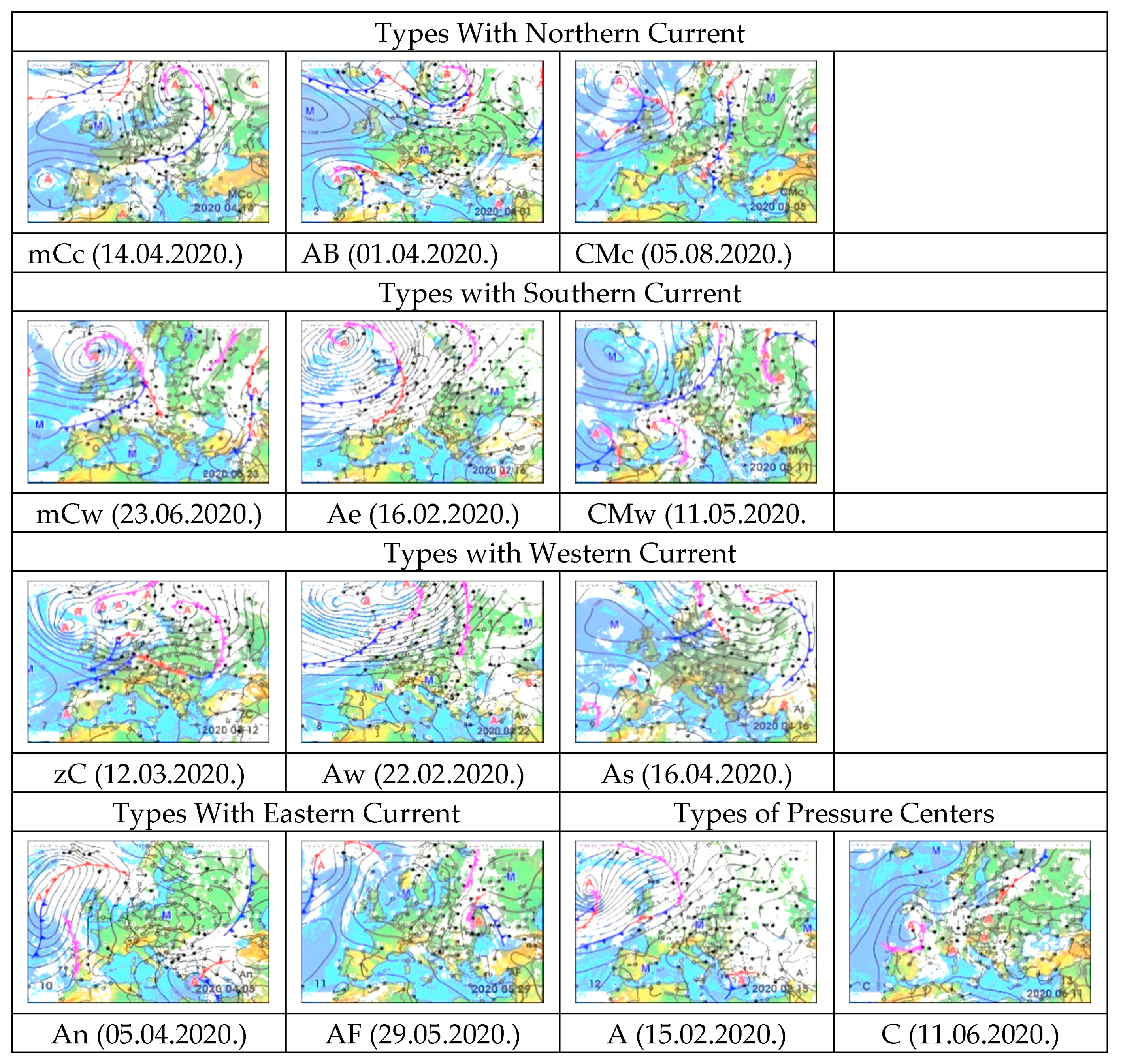
| Meridional Types | Zonal and Central Types |
|---|---|
| Types Connected with Western Current: | |
| Types Connected with Northern Current: | zC—zonal flow, slightly cyclonic influence |
| mCc—Hu is in the rear of a West-European cyclone | Aw—anticyclone extending from the west |
| AB—anticyclone over the British Isles | As—anticyclone to the south from Hungary |
| CMc—Hu is in the rear of a Mediterranean cyclone | Types Connected with Eastern Current: |
| An—anticyclone to the north from Hungary | |
| Types Connected with Southern Current: | AF—anticyclone over Fenno-Scandinavia |
| mCw—Hu is in the fore of a West-European cyclone | Types of Pressure Centers: |
| Ae—anticyclone to the east from Hungary | A—anticyclone center over Hungary |
| CMw—Hu is in the fore of a Mediterranean cyclone | C—cyclone center over Hungary |
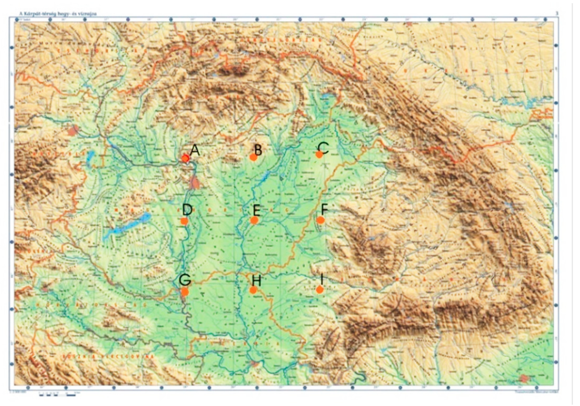
| Variable | Month | A | B | C | D | E | F | G | H | I |
|---|---|---|---|---|---|---|---|---|---|---|
| High Preci-pitation (mm/day) | Jan | 5.1 | 8.6 | 5.2 | 5.1 | 3.9 | 4.2 | 4.7 | 3.9 | 6.9 |
| Apr | 12.1 | 15.3 | 8.6 | 8.7 | 8.2 | 8.8 | 7.5 | 9.9 | 9.7 | |
| July | 19.3 | 21.3 | 16.6 | 15.4 | 18.2 | 15.3 | 13.8 | 16.2 | 14.2 | |
| Oct | 9.4 | 14.8 | 11.4 | 7.5 | 7.3 | 7.2 | 6.3 | 6.7 | 9.8 | |
| High Tmax (°C) | Jan | 8.9 | 2.6 | 3.8 | 8.4 | 6.1 | 4.9 | 6.6 | 9.5 | 10.9 |
| Apr | 20.1 | 10.3 | 16.3 | 22.0 | 18.4 | 18.0 | 21.9 | 23.9 | 23.6 | |
| July | 27.9 | 18.6 | 24.9 | 29.7 | 26.1 | 26.5 | 30.0 | 31.9 | 32.1 | |
| Oct | 20.4 | 15.1 | 17.6 | 21.5 | 17.7 | 18.7 | 20.8 | 23.2 | 22.9 | |
| Low Tmin (°C) | Jan | −18.8 | −22.1 | −20.7 | −20.2 | −22.7 | −18.6 | −20.1 | −17.9 | −13.2 |
| Apr | −2.4 | −9.9 | −6.3 | −2.2 | −6.1 | −4.6 | −2.4 | −0.7 | −0.5 | |
| July | 8.2 | 2.6 | 4.2 | 8.7 | 5.5 | 7.2 | 9.0 | 10.8 | 9.4 | |
| Oct | −2.8 | −8.6 | −6.8 | −3.2 | −6.1 | −4.4 | −3.1 | −1.9 | −1.4 | |
| Strong Wind (m/s) | Jan | 8.2 | 6.2 | 5.4 | 9.7 | 11.2 | 8.8 | 12.7 | 8.1 | 7.2 |
| Apr | 5.2 | 8.2 | 6.3 | 7.6 | 7.1 | 8.6 | 8.6 | 7.5 | 7.9 | |
| July | 4.3 | 6.4 | 4.9 | 5.7 | 7.0 | 6.5 | 6.8 | 6.5 | 5.5 | |
| Oct | 6.0 | 7.0 | 5.2 | 7.4 | 7.8 | 7.2 | 8.6 | 6.7 | 5.9 |
| Variable | Month | A | B | C | D | E | F | G | H | I |
|---|---|---|---|---|---|---|---|---|---|---|
| High Preci-pitation (mm/day) | Jan | 21.0 | 40.0 | 15.8 | 23.8 | 18.0 | 15.6 | 19.6 | 18.7 | 35.5 |
| Apr | 53.7 | 56.8 | 21.4 | 40.7 | 45.7 | 37.6 | 31.8 | 40.3 | 41.0 | |
| July | 98.3 | 74.0 | 50.0 | 64.5 | 82.0 | 74.5 | 103.6 | 66.0 | 57.2 | |
| Oct | 37.8 | 52.8 | 39.0 | 39.7 | 27.7 | 27.8 | 34.6 | 28.9 | 40.5 | |
| High Tmax (°C) | Jan | 13.8 | 7.8 | 8.5 | 14.7 | 11.4 | 9.5 | 12.3 | 15.9 | 16.9 |
| Apr | 25.3 | 15.0 | 20.2 | 27.2 | 22.6 | 23.4 | 26.8 | 28.8 | 28.4 | |
| July | 33.1 | 23.2 | 28.9 | 34.8 | 30.8 | 31.4 | 34.2 | 37.2 | 38.6 | |
| Oct | 25.8 | 19.5 | 22.3 | 27.7 | 24.2 | 24.5 | 27.0 | 29.9 | 26.3 | |
| Low Tmin (°C) | Jan | −26.7 | −32.4 | −32.1 | −32.2 | −33.3 | −29.8 | −31.4 | −28.9 | −23.0 |
| Apr | −8.4 | −15.2 | −12.1 | −10.2 | −14.0 | −9.0 | −11.3 | −10.2 | −5.3 | |
| July | 4.9 | −0.6 | 0.6 | 5.7 | 2.2 | 4.0 | 5.9 | 8.0 | 4.6 | |
| Oct | −8.6 | −15.6 | −15.5 | −9.9 | −14.6 | −11.4 | −9.0 | −7.4 | −9.4 | |
| Strong Wind (m/s) | Jan | 15.6 | 14.0 | 14.5 | 19.5 | 28.3 | 21.4 | 26.7 | 32.4 | 15.5 |
| Apr | 12.0 | 17.3 | 11.2 | 14.9 | 16.2 | 14.5 | 17.4 | 14.8 | 15.1 | |
| July | 12.7 | 14.1 | 10.1 | 19.1 | 21.7 | 19.6 | 21.3 | 20.3 | 10.1 | |
| Oct | 17.0 | 17.2 | 12.5 | 19.2 | 22.4 | 19.0 | 21.5 | 16.7 | 15.2 |
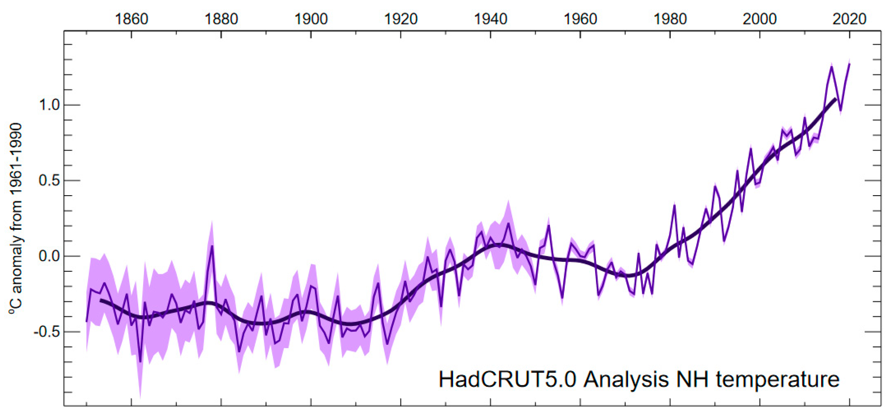
| Periods | Duration | Correlation | Regression (°C/10 Years) | NH Trend |
|---|---|---|---|---|
| 1881–1910 | 30 years | 0.002 | 0.0002 | neutral |
| 1911–1940 | 30 years | 0.843 | 0.20 | warming |
| 1941–1970 | 30 years | −0.503 | −0.07 | cooling |
| 1971–2020 | 50 years | 0.954 | 0.28 | warming |
| Type | Jan | Feb | Mar | Apr | May | June | July | Aug | Sep | Oct | Nov | Dec | Year |
|---|---|---|---|---|---|---|---|---|---|---|---|---|---|
| mCc | 11 | 13 | 14 | 19 | 21 | 17 | 18 | 14 | 16 | 16 | 16 | 10 | 16 |
| AB | 8 | 6 | 11 | 8 | 8 | 11 | 7 | 6 | 7 | 6 | 5 | 6 | 8 |
| CMc | 1 | 1 | 1 | 2 | 1 | 1 | 1 | 1 | 1 | 1 | 2 | 1 | 1 |
| mCw | 9 | 9 | 9 | 6 | 5 | 4 | 2 | 2 | 5 | 5 | 6 | 8 | 5 |
| Ae | 12 | 12 | 13 | 11 | 7 | 7 | 7 | 9 | 13 | 18 | 23 | 14 | 12 |
| CMw | 9 | 9 | 7 | 10 | 6 | 4 | 2 | 2 | 5 | 7 | 12 | 12 | 7 |
| zC | 4 | 3 | 3 | 1 | 0 | 0 | 1 | 0 | 1 | 2 | 2 | 4 | 2 |
| Aw | 12 | 14 | 12 | 8 | 9 | 17 | 23 | 18 | 14 | 9 | 9 | 12 | 13 |
| As | 8 | 7 | 4 | 4 | 5 | 4 | 3 | 2 | 3 | 5 | 5 | 7 | 4 |
| An | 10 | 7 | 9 | 11 | 14 | 9 | 10 | 16 | 13 | 9 | 5 | 7 | 10 |
| AF | 1 | 5 | 4 | 7 | 8 | 5 | 6 | 8 | 7 | 7 | 2 | 3 | 6 |
| A | 14 | 11 | 10 | 7 | 9 | 14 | 14 | 16 | 12 | 12 | 11 | 15 | 12 |
| C | 2 | 3 | 4 | 6 | 6 | 7 | 6 | 4 | 4 | 3 | 2 | 2 | 4 |
| All | 100 | 100 | 100 | 100 | 100 | 100 | 100 | 100 | 100 | 100 | 100 | 100 | 100 |
| Original Circulation Types (Frequency from 13 Types) | |||||
|---|---|---|---|---|---|
| Significance according to | Winter | Spring | Summer | Autumn | Percentage |
| Correlation | 4 | 6 | 5 | 4 | 37% |
| Regression | 4 | 6 | 5 | 4 | 37% |
| Significance in | NH Correl. | Winter | Spring | Summer | Autumn | Percent |
|---|---|---|---|---|---|---|
| 1881–1910 | 0.002 | 1 | 2 | 0 | 3 | 12% |
| 1911–1940 | 0.843 | 2 | 1 | 1 | 1 | 10% |
| 1941–1970 | −0.503 | 0 | 4 | 2 | 1 | 13% |
| 1971–2020 | 0.954 | 4 | 6 | 5 | 4 | 37% |
| Circulation Types Found Significant in 1971–2020 | Frequency Trend (yr−1) 1881–1910 R(TNH) = 0.002 | Frequency Trend (yr−1) 1911–1940 R(TNH) = 0.843 | Frequency Trend (yr−1) 1941–1970 R(TNH) = −0.503 | Frequency Trend (yr−1) 1971–2020 R(TNH) = 0.954 | |
|---|---|---|---|---|---|
| Winter | mCc | +0.228 | |||
| CMc | +0.086 | −0.045 | |||
| Ae | −0.196 | ||||
| An | −0.132 | ||||
| Spring | mCc | +0.331 | |||
| CMc | +0.100 | −0.101 | |||
| mCw | −0.123 | ||||
| Ae | −0.335 | −0.098 | |||
| CMw | +0.233 | +0.073 | −0.071 | ||
| zC | −0.065 | ||||
| Summer | mCc | +0.242 | |||
| CMc | +0.109 | −0.045 | |||
| mCw | −0.081 | ||||
| CMw | −0.069 | ||||
| zC | −0.907 | ||||
| Autumn | mCc | +0.358 | |||
| CMc | −0.047 | ||||
| zC | −0.040 | ||||
| Aw | −0.236 | −0.096 |
Publisher’s Note: MDPI stays neutral with regard to jurisdictional claims in published maps and institutional affiliations. |
© 2021 by the authors. Licensee MDPI, Basel, Switzerland. This article is an open access article distributed under the terms and conditions of the Creative Commons Attribution (CC BY) license (https://creativecommons.org/licenses/by/4.0/).
Share and Cite
Mika, J.; Károssy, C.; Lakatos, L. Variations in the Peczely Macro-Synoptic Types (1881–2020) with Attention to Weather Extremes in the Pannonian Basin. Atmosphere 2021, 12, 1071. https://doi.org/10.3390/atmos12081071
Mika J, Károssy C, Lakatos L. Variations in the Peczely Macro-Synoptic Types (1881–2020) with Attention to Weather Extremes in the Pannonian Basin. Atmosphere. 2021; 12(8):1071. https://doi.org/10.3390/atmos12081071
Chicago/Turabian StyleMika, János, Csaba Károssy, and László Lakatos. 2021. "Variations in the Peczely Macro-Synoptic Types (1881–2020) with Attention to Weather Extremes in the Pannonian Basin" Atmosphere 12, no. 8: 1071. https://doi.org/10.3390/atmos12081071