Article

Low-Cost Air Quality Stations’ Capability to Integrate Reference Stations in Particulate Matter Dynamics Assessment

by
Lorenzo Brilli
1,
Federico Carotenuto
1,*,
Bianca Patrizia Andreini
2,
Alice Cavaliere
1,
Andrea Esposito
3,
Beniamino Gioli
1,
Francesca Martelli
1,
Marco Stefanelli
2,
Carolina Vagnoli
1,
Stefania Venturi
4,5,
Alessandro Zaldei
1 and
Giovanni Gualtieri
1
1
CNR-IBE, National Research Council Institute for the BioEconomy, Via Caproni 8, 50145 Firenze, Italy
2
ARPAT, Tuscany Region Environmental Protection Agency, Via Porpora, 22, 50144 Firenze, Italy
3
CNR-ISAFOM, National Research Council Institute of Mediterranean Agricultural and Forestry Systems, P. le Enrico Fermi 1—Loc. Porto del Granatello, 80055 Portici, Italy
4
DST-Unifi, Department of Earth Sciences, University of Florence, Via G. La Pira 4, 50121 Firenze, Italy
5
CNR-IGG, National Research Council Institute of Geosciences and Earth Resources, Via G. La Pira 4, 50121 Firenze, Italy
*
Author to whom correspondence should be addressed.
Atmosphere 2021, 12(8), 1065; https://doi.org/10.3390/atmos12081065
Submission received: 3 July 2021 / Revised: 10 August 2021 / Accepted: 16 August 2021 / Published: 19 August 2021
(This article belongs to the Special Issue PM Sensors for the Measurement of Air Quality)

Abstract

:
Low-cost air quality stations can provide useful data that can offer a complete picture of urban air quality dynamics, especially when integrated with daily measurements from reference air quality stations. However, the success of such deployment depends on the measurement accuracy and the capability of resolving spatial and temporal gradients within a spatial domain. In this work, an ensemble of three low-cost stations named “AirQino” was deployed to monitor particulate matter (PM) concentrations over three different sites in an area affected by poor air quality conditions. Data of PM2.5 and PM10 concentrations were collected for about two years following a protocol based on field calibration and validation with a reference station. Results indicated that: (i) AirQino station measurements were accurate and stable during co-location periods over time (R2 = 0.5–0.83 and RMSE = 6.4–11.2 μg m−3; valid data: 87.7–95.7%), resolving current spatial and temporal gradients; (ii) spatial variability of anthropogenic emissions was mainly due to extensive use of wood for household heating; (iii) the high temporal resolution made it possible to detect time occurrence and strength of PM10 concentration peaks; (iv) the number of episodes above the 1-h threshold of 90 μg m−3 and their persistence were higher under urban and industrial sites compared to the rural area.

1. Introduction

Citizen participation in public debates on life quality is greatly increasing. Topics such as environmental monitoring and related scientific activities are attracting increasing interest. Such interest is strong for those citizens living in the most urbanized areas, where industrial activities, heavy traffic, and intense heating usage are the most critical sources of air pollution. Such emissions affect public air quality and, in turn, health conditions [1,2,3,4]. In Europe, despite the decreasing trend since 2000, the percentage of the urban population exposed to pollutant levels above EU standards remains relevant. In 2018, for example, 34% of urban citizens were exposed to ozone and 15% to PM10 levels above the EU limit values [5].
Air pollution levels are generally sampled and measured by fixed air quality stations following a reference method in accordance with the regulatory procedure, e.g., in Europe, by the 2008/50/EC Directive [6], and managed by regional or national environmental protection agencies. Despite their high degree of accuracy, these stations, from here onwards named as “reference stations”, are affected by high costs of procurement and maintenance, limiting their number over the territory. Furthermore, by complying with the official regulations (e.g., [6]), the observations are reported at low time-frequency, ranging from hourly (gas species) to daily (particulate matter, PM). As for the latter, several studies [7,8,9,10] have demonstrated how the availability of sub-daily (e.g., hourly) observations enables a more insightful investigation of PM dynamics across the day, thus leading to a better understanding of the role played by emission sources and meteorological conditions. To capture the actual spatial-temporal air quality variability, measurements from fixed stations may be integrated with “indicative measurements” [11] provided by low-cost air quality stations, which have a small size and low power consumption. Such characteristics make them appealing in situations where traditional monitors are unfeasible [12]. The possibility to install such stations over urban buildings, private houses, and industries, would contribute to the creation of citizens’ observatories [13,14]. Such observatories would allow citizens to gain information on air quality levels of their own city, thus raising awareness on environmental issues and sharing of environmental decision making.
In the present study, an air quality monitoring campaign was carried out by using innovative low-cost air quality stations, named “AirQino”, developed by CNR-IBE and equipped with sensors for collecting main atmospheric pollutants [15,16]. The municipality of Capannori, located near the city of Lucca (Italy), was chosen as a testing area. Capannori is a small town but is affected by air pollution levels relatively higher than those involving much more urbanized areas of the region [17]. It is impacted by a variety of emission sources and lies in a plain area affected by weather conditions unfavorable to air pollutant dispersion. The study was focused on PM concentrations, a well-known long-term issue affecting the area [18,19], in order to provide supplementing air quality measurements to fixed measurements collected by the official monitoring network. AirQino low-cost air quality stations collected data in the area for about two years. This study has the objectives of assessing the followings regarding such stations: (i) their accuracy and temporal stability by co-locating them with the reference station in different periods and both in calibration and validation modes; (ii) their capacities to resolve spatial and temporal gradients present in a polluted area within measurement accuracy, as a pre-requisite for any forthcoming larger-scale network deployment; (iii) their capability to assess short-term (i.e., 1-h) population exposure to critical PM10 concentrations that traditional stations, returning solely the PM10 daily value, are unable to deliver.

2. Materials and Methods
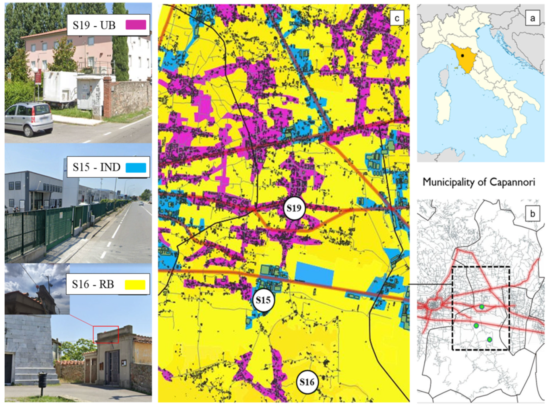
2.1. Study Area

The study area was in Capannori (43°52′ N, 10°34′ E), a rural town close to the city of Lucca and located in the western part of the Tuscany region (Italy). The surface area of Capannori municipality (156 km2) is remarkable if compared to its resident population (about 46,500 inhabitants), thus resulting in a population density of 298 inhabit./km2. Capannori was firstly chosen because of its remarkable air pollution problems and particularly high PM concentrations. Outcomes from the PATOS regional project [18], various Tuscany region reports [17], and scientific studies [19] reveal that the area is the most polluted among all sampling sites throughout the Tuscany region, with annual PM10 concentrations and number of daily exceedances higher than those registered over other much more urbanized areas of the region. Secondly, this area was selected since it is impacted by quite heterogeneous emission sources, including one major highway, local roads massively traveled by heavy-duty vehicles, combustion plants for paper transformation, extensive use of wood for household heating, and agricultural waste burning including biomass burning [20]. In addition, air pollutant dispersion in the area is hampered by adverse winter weather conditions such as low wind regime, stable atmospheric conditions, and shallow thermal inversions [21]. Therefore, since it is influenced by different air pollution sources throughout its territory, Capannori offered the opportunity to assess the capability of the developed low-cost air quality stations over differently polluted sites.

2.2. The AirQino Monitoring Unit

The AirQino monitoring unit, developed by CNR-IBE within the national SMARTCITIES project [15,16], consists of an Arduino Shield Compatible electronic board equipped with low-cost and high-resolution sensors (2–3 min data acquisition frequency) providing measurements of air pollutants concentrations including PM2.5 and PM10. The AirQino board can work as an Arduino shield that can access data through the PD2 (TX) and PD3 (RX) ports and provide the 5 V power supply. The particulate matter sensor for PM2.5 and PM10 are based on the Novasense SDS011 detector (Inovafitness, Jinan, China). The SDS011, based on the principle of laser scattering, provides PM concentrations directly in µg/m−3 due to pre-processing from the manufacturer. The board microprocessor collects the readings from all installed sensors and sends them to a data server via a general packet radio service (GPRS) connection. Data can then be visualized in real time through a dedicated web interface [14]. Further details can be found in [22].

2.3. Air Pollution Zones and Station Deployment

The main idea behind the creation of this experiment focused on taking advantage of the air pollution heterogeneity within Capannori municipality to test the monitoring capability of AirQino stations under different air quality conditions. The choice of the station area deployment was driven by:
i.
A land-use analysis of the municipality based on the most updated (2018) Corine Land Cover (CLC) classification [23], where the highest third disaggregation level (including 44 classes) was considered (Figure S1).
ii.
The current regulations for air pollution. According to the fixed air quality measurement classification stated by the 2008/50/EC EU Directive [6], a total of nine monitoring station types can generally be identified as a combination of: (i) site characteristics (urban, suburban, rural); and (ii) prevailing emission category (road traffic, industrial activities, background).
Consequently, CLC classification of the area (point ‘i’) was adjusted in order to fit the above station classification (point ‘ii’), thus theoretically returning a total of nine air pollution zones. The result of this analysis is shown in Figure 1, where four areas representing different air pollution conditions—and thus air quality stations—were detected: (i) urban–background (UB, purple areas); (ii) urban–traffic (UT, red areas); (iii) rural–background (RB, yellow areas); (iv) industrial (IND, blue areas).
Three AirQino stations were deployed over three different air pollution zones (Figure 1):
  • The S15 station was located in the southern–central part of the municipality, an area where the main emission contributions are likely derived from industrial activities (43°49′2460″ N, 10°33′4580″ E). S15 was therefore classified as an IND station and conveniently renamed S15-IND. Its observation period was 28 June 2018–15 April 2020.
  • The S16 station was located in the southern part of the municipality, a rural area not significantly affected by nearby emission sources (43°49′2460″ N, 10°33′4580″ E). S16 was therefore classified as an RB station and renamed S16-RB. Its observation period was 28 June 2018–15 April 2020.
  • The S19 station was co-located by the Regional Agency for Environmental Protection of Tuscany (ARPAT) reference station, deployed in the central part of the municipality (43°50′2340″ N, 10°34′2241″ E). Similar to the ARPAT reference station, S19 was classified as a UB station and renamed S19-UB. Its observation period was 19 January 2018–15 April 2020.
According to [20], total emissions of primary PM10 and PM2.5 over the municipality of Capannori were ascribed to heating systems to an extent of 86.9 and 90.7%, respectively, while they were attributed to road traffic to an extent of 9.5 and 8.7%. Therefore, no UT location was selected for the deployment of AirQino stations in the area. Characteristics of all installed stations are summarized in Table S1. The low-cost stations were continuously in operation for 2 years and 3 months (S19-UB), and 1 year and 9 months (S15-IND and S16-RB). Their receptor points were located at heights ranging between 2.5 and 3.5 m above ground level.

2.4. Calibration and Validation

After almost one year of measurements, all AirQino stations were co-located beside the ARPAT reference station, from 22 March 2019 to 7 June 2019, to undergo field calibration. The ARPAT station employed a dual-channel filter-based gravimetric sampling method [24]. The AirQino raw data during co-location were processed according to three steps: (i) despiking according to an interquartile range-based algorithm, where outliers were defined as values below (above) the first (third) quartile minus (plus) three times the interquartile range; (ii) manual cleaning for deleting outliers not detected by the automatic despiking procedure; (iii) creation of timing coherence among all three AirQino stations. Specifically, a linear regression procedure was applied only using concentration as an independent variable. Then, since observations from the reference station were only available at a daily time scale, high-resolution AirQino data were daily averaged (after despiking and manual cleaning) and compared against the reference daily data in order to detect their relationship. The obtained field calibration coefficients were finally applied to each AirQino station (S15, S16, and S19) for their whole high-resolution dataset.
After the field calibration procedure, all AirQino stations were validated on-site for the period 25 January 2020–20 February 2020, when all stations were co-located once again beside the ARPAT reference station. This procedure was done to assess air quality station robustness and to evaluate measurement uncertainties due to different sensors drifts through time.

2.5. Data Processing and Statistical Analysis

Statistical analyses evaluating the performances of each AirQino station during both field calibration and field validation procedures were applied with the software MatLab (R2019a) using ANOVA, coefficient of determination (R2, Equation (1)) and root mean square error (RMSE, Equation (2)). In the two equations, N represents the number of predictions/observations; pi predictions; oi observations; p ¯ i mean of predictions; o ¯ i mean of observations.
R 2 = i = 1 N p i p ¯ i 2 i = 1 N o i o ¯ i 2
R M S E = i = 1 N p i o i 2 N
Yearly and monthly patterns, seasonal and daily courses, and high-frequency (1-h, 30-min, and 10-min) dynamics of PM2.5 and PM10 concentrations for 2018–2019 and 2019–2020 periods were assessed over the three areas.
Finally, short-term population exposure was evaluated at high resolution (1 h) following the approach proposed by [25], which considers exceedances of 1-h threshold concentrations of 90 µg m−3 as a good predictor of exceedances of the PM10 daily limit value (50 µg m−3). The analysis was carried out for the period 28 June 2018–15 April 2020 while excluding the co-location sub-periods. Periods of data sources for the different activities were reported in Table 1.

3. Results

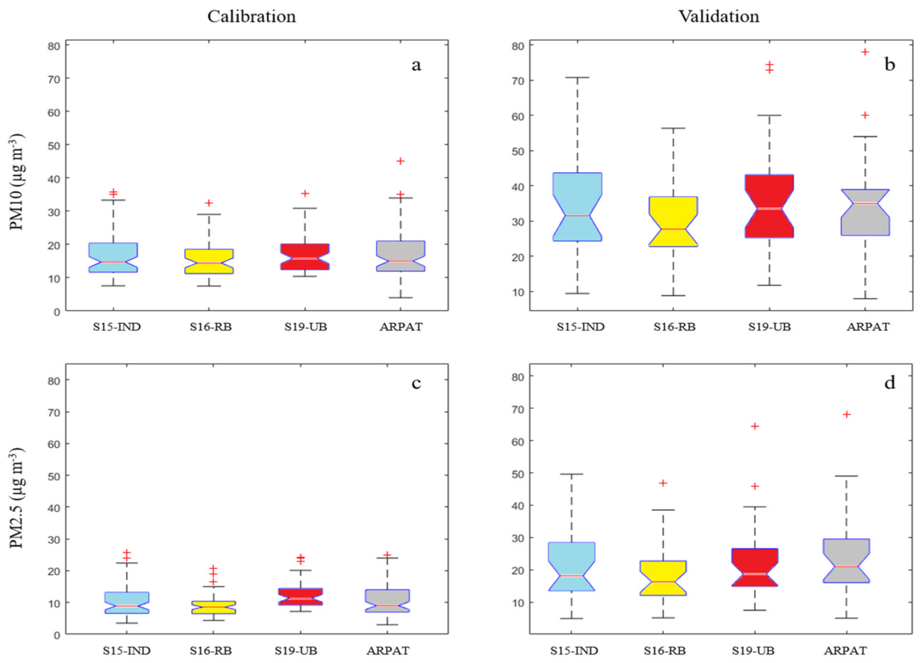
3.1. Stations Field Calibration and Field Validation

Daily data were used for field calibration and validation for maintaining time coherence with reference stations. The daily measured concentrations of PM10 and PM2.5 are available from the ARPAT website (http://www.arpat.toscana.it/temi-ambientali/aria/qualita-aria, accessed on 25 March 2021). The results of field calibration between the AirQino stations and the ARPAT reference station showed R2 = 0.54 − 0.85 and RMSE = 2.3 − 4.6 µg m−3 (Table 2, Figure S2). The highest performances were shown by S15-IND for both PM10 (R2 = 0.74, RMSE = 4.14 µg m−3) and PM2.5 (R2 = 0.85, RMSE = 2.28 µg m−3), while the lowest were shown by S19-UB for both PM10 (R2 = 0.63, RMSE = 4.6 µg m−3) and PM2.5 (R2 = 0.54, RMSE = 4.25 µg m−3).
A general agreement between the AirQino stations and the ARPAT station was also achieved during field validation (R2 = 0.50 − 0.83 and RMSE = 7.5 − 11.2 µg m−3, Table 1). The best scores were again reported by S15-IND for both PM10 (R2 = 0.74, RMSE = 7.54 µg m−3) and PM2.5 (R2 = 0.83, RMSE = 6.41 µg m−3), while the worst by S19-UB for both PM10 (R2 = 0.50, RMSE = 11.24 µg m−3) and PM2.5 (R2 = 0.56, RMSE = 9.65 µg m−3). An additional analysis was performed to test whether the correlation between AirQino and reference stations was affected by meteorological effects, applying two regression models considering air temperature and relative humidity in addition to PM10 concentration or considering only air temperature and relative humidity as regressors. This analysis revealed that air temperature and relative humidity were overall not capable to explain the relationship between the AirQino and reference stations (Table S2). We furthermore explored the dependence between AirQino stations on meteorological information by calculating the correlation coefficient between the PM10 percentage error and either air temperature or relative humidity. The percentage error was calculated between AirQino daily averages and ARPAT data for a dataset combining both co-location periods. No major dependence of sensor performance was seen for any AirQino for either temperature (R2 ranging between 0.01 and 0.07) or relative humidity (R2 ranging between 0.01 and 0.23) (Table S3).
Performances of AirQino stations under both field calibration and field validation processes were also assessed through a boxplot analysis (Figure 2). For PM10 concentrations, no appreciable change occurred during the calibration between ARPAT (Median = 15 µg m−3) and AirQino stations (Median = 14.7, 14.45, and 15.8 µg m−3 for S15-IND, S16-RB and S19-UB, respectively, Figure 2a). A similar outcome was observed during the validation, where, however, the median value of ARPAT was slightly higher (35 µg m−3), as well as the interquartile range compared to AirQino stations (Median = 31.5, 27.7 and 33.7 µg m−3 for S15-IND, S16-RB, and S19-UB, respectively, Figure 2b). PM2.5 concentrations exhibited a similar pattern to PM10 concentrations for both calibration and validation, yet with a lower magnitude (Figure 2c,d).
An ANOVA analysis was also performed, eventually showing that no AirQino station exhibited significant differences from the ARPAT reference station (Figure S3). For the whole dataset, a valid data coverage of 24-h observations ranging from 87.7% to 95.7% was observed (Table S1).

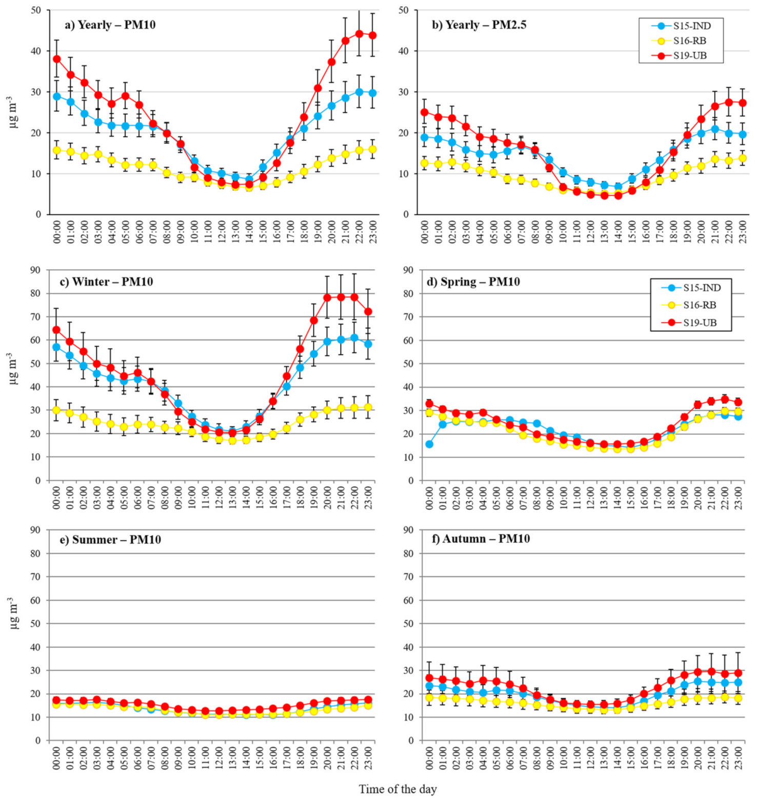
3.2. Annual and Seasonal Concentrations

Monthly statistics of PM10 and PM2.5 concentrations of ARPAT and AirQino stations are summarized in Table 3. The pattern showed the highest PM10 and PM2.5 values during the wintertime, while the lowest were observed during the summer months for both ARPAT reference stations and all AirQino stations. From May to September all air quality stations showed very low PM concentrations, ranging from 10 to 20 µg m−3 for PM10 and from 7 to 12 µg m−3 for PM2.5. The highest average monthly concentrations were observed in winter, with PM10 concentrations higher than 30 µg m−3 and PM2.5 concentrations higher than 20 µg m−3 observed by almost all stations (Table 2). In particular, the highest average monthly concentrations were found in January for both PM10 (76.6 ± 33.3, 57.6 ± 26.0 and 61.4 ± 31.7 µg m−3) and PM2.5 (67.9 ± 30.8, 40.0 ± 17.2 and 40.5 ± 22.2 µg m−3) by ARPAT, S15-IND and S19-UB stations, respectively. The monthly yearly average PM10 concentrations did not exhibit considerable differences between the ARPAT reference station (32.1 ± 12.1 µg m−3) and the co-located S19-UB (27.7 ± 11.3 µg m−3), while a lower value was observed in the rural area (S16-RB; 18.4 ± 6.6 µg m−3). A similar pattern was also observed for PM2.5 concentrations, where, however, the monthly yearly average PM2.5 concentrations of the co-located S19-UB tended to underestimate (17.6 ± 7.2 µg m−3) that reported by the ARPAT reference station (24.1 ± 10.3 µg m−3).
High-resolution PM2.5 and PM10 concentrations observed by the AirQino stations across the whole study period have been hourly averaged in order to achieve an overall daily cycle (Figure 3).
To maintain data coherency between the three locations, the analysis was carried out for the period 28 June 2018–15 April 2020 while excluding the co-location periods (i.e., field calibration and validation, see Table 1).
The yearly daily cycles of hourly averaged PM10 and PM2.5 concentrations showed a similar pattern for all stations, with the highest values occurring from late afternoon to early morning and the lowest values during the warmest hours of the day (Figure 3a,b). This pattern was more pronounced for S19-UB and S15-IND, where concentrations from late afternoon to early morning were almost twice as S16-RB. The pattern of PM2.5 concentrations was similar to the one observed for PM10 for all AirQino stations, but with a lower magnitude.
Strong differences were observed in the seasonal daily cycles of hourly averaged PM10 concentrations, with the most marked daily variations occurring in winter (Figure 3c) and the least in summer (Figure 3e). In winter, PM10 concentrations tended to increase from the afternoon (17:00) to early night (23:00), then slowly decreasing to early morning, particularly for S15-IND and S19-UB, whose concentrations almost doubled those observed by S16-RB. In spring (Figure 3d) and particularly in summer (Figure 3e), the pattern of PM10 concentrations was flat, with no appreciable difference between the stations, while in autumn (Figure 3f) two early morning and late evening weak peaks may be observed, markedly for S15-IND concentrations.

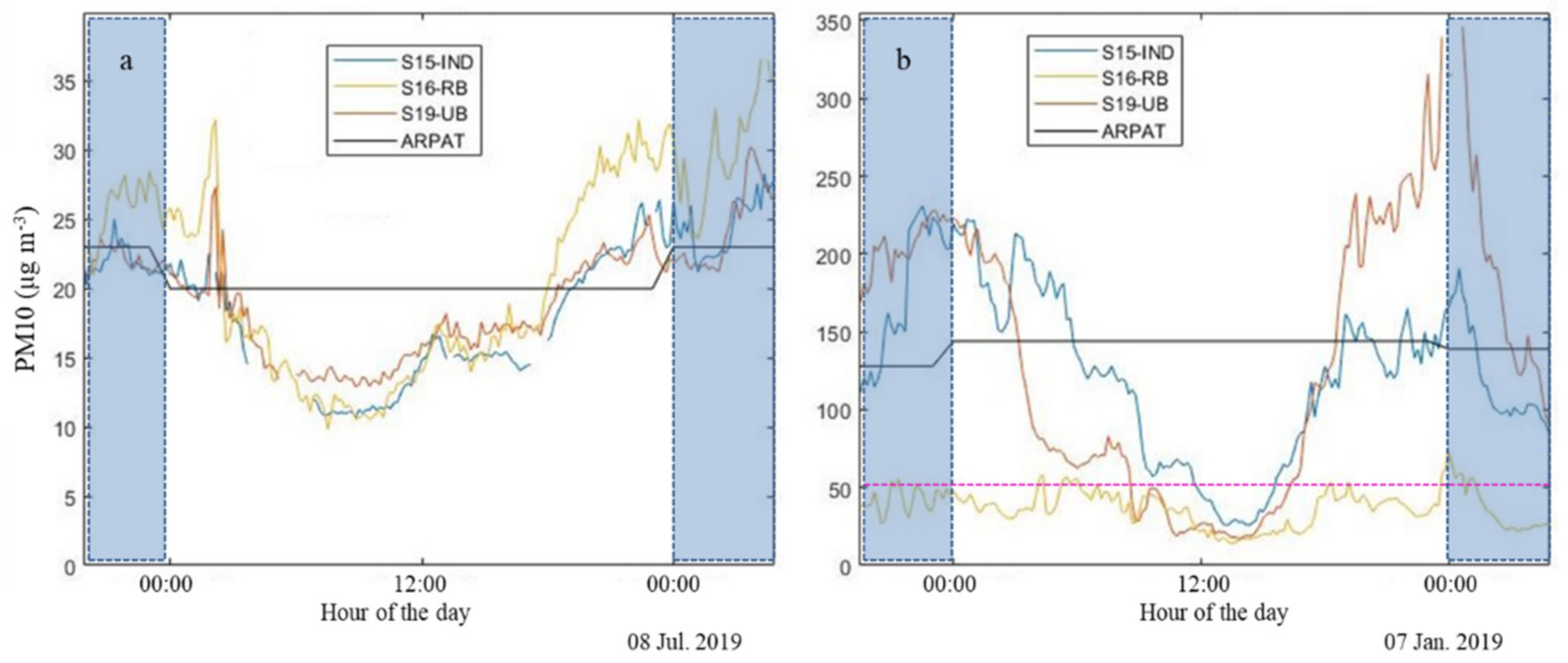
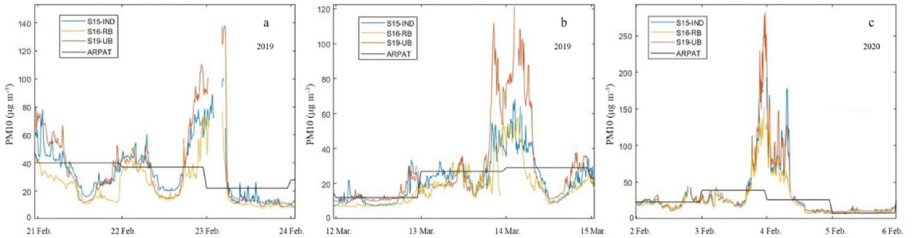
3.3. Wintertime PM10 Concentrations

Specific attention was paid to the 2018–2019 and 2019–2020 winter periods by analyzing the daily time series of PM10 concentrations (Figure 4). As mentioned above, field validation data (25 January–20 February 2020) were excluded by this analysis.
Pattern and magnitude exhibited by both S15-IND and S19-UB stations were similar to those provided by the ARPAT reference station, with the highest PM10 concentrations (above 100 µg m−3) observed during the holiday period between the end of December and the beginning of January. During the 2018–2019 winter period, the overall average values of PM10 concentrations for S19-UB (45.7 µg m−3) and S15-IND (44.0 µg m−3) were lower than that measured by ARPAT (61.3 µg m−3), while during the 2019–2020 winter period the observations by S19-UB (46.9 µg m−3) and S15-IND (40.4 µg m−3) were more consistent with the values measured by ARPAT (52.2 µg m−3). By contrast, S16-RB showed a similar pattern but a significantly lower magnitude across the two periods. During the period 25 January–20 February 2020, all AirQino stations were co-located by the ARPAT reference station for field validation (Figure 4, blue shaded area); consistently, they showed similar pattern and magnitude both between themselves and against the ARPAT station. The average values of PM10 concentrations observed by S16-RB during the 2018–2019 and 2019–2020 winter periods were 21.5 and 27.0 µg m−3, respectively.

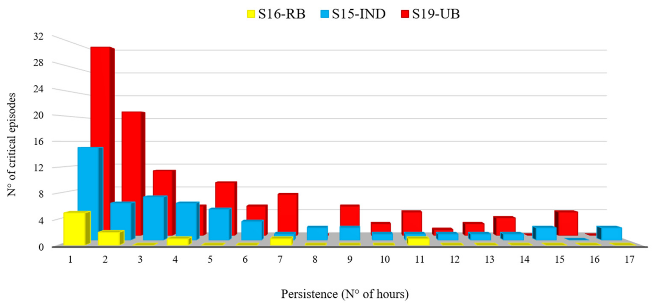
3.4. PM10 Concentration High-Frequency Analysis and Population Critical Exposure

The high-frequency (1-h, 30-min, and 10-min) analysis of AirQino-provided observations returned information that reference stations—solely providing 24-h concentrations as determined by the EU directive—are usually unable to return. In Figure 5, two examples of PM10 concentrations during summer and a typical winter day at 10-min vs. 24-h frequency are reported. In summer (Figure 5a), the dynamics of 10-min PM10 concentrations, denoting a clear coherence between all AirQino stations, showed a U-shape pattern characterized by a very low variability (ranging about 10–30 µg m−3) that the reference station was unable to capture. In winter (Figure 5b), a similar U-shape pattern is exhibited by the AirQino stations, but with much higher variability, particularly for S15-IND and S19-UB stations. Furthermore, except for the hours around noon, S15-IND and S19-UB stations record PM10 concentrations steadily above the daily limit value (50 µg m−3, purple dotted line). By contrast, S16-RB does not show the same high variability, with PM10 concentrations almost steadily below the daily limit value.
The 10-min analysis also showed the capability of S15-IND, S16-RB, and S19-UB stations to detect time occurrence and relative strength of PM10 concentration peaks that the reference station was unable to capture (Figure 6). The 10-min peaks, observed by all AirQino stations when co-located (Figure 6c) as well as when not (Figure 6a,b), were steadily higher than the daily limit value and then ARPAT daily values.
Furthermore, short-term population exposure was calculated following the approach proposed by [25]. The analysis was carried out for the period 28 June 2018–15 April 2020 while excluding the co-location sub-periods. AirQino stations registered a total of 13,224 hourly values, with data availability ranging from 82.2% for S15-IND to 95.1 for S19-UB (Table 4). The total number of 1-h PM10 concentrations above 90 µg m−3 was 280, 31, and 504 h for S15-IND, S16-RB (Table 4), which corresponded to the 2.6%, 0.2%, and 4% of hours of the whole available dataset for each site (Table 3).
In addition, the persistence of PM10 high-resolution critical concentrations was evaluated by calculating the number of consecutive hours with PM10 concentrations higher than 90 µg m−3, named as “critical episodes”. The total number of such critical episodes was 56, 10, and 111 for S15 -IND, S16-RB, and S19-UB, respectively, mainly occurring in winter (e.g., December and January, see Table 4).
The results indicated that most of the critical episodes had low persistence (1–5 consecutive hours). The highest persistence was found in both urban and industrial areas, with more than one episode with 15–17 consecutive hours exceeding 90 µg m−3. By contrast, in the rural area, only two single episodes with 7 and 11 consecutive hours with PM10 concentrations above 90 µg m−3 were observed (Figure 7).

4. Discussion

The AirQino stations proved to be a robust tool for investigating air quality dynamics at high spatial and temporal scales. Installed over three areas with different urbanization and land use characteristics, and periodically co-located with a reference station, the low-cost stations measured significantly different air quality conditions and not significantly different values at the reference site, confirming the why behind a larger-scale network distribution. Considering the whole dataset, the stations provided a valid data percent between 87.7 and 95.7% (Table S1) out of a 24-h observation period. As graphically (Figure 4) and statistically (Table 2) proven, the on-site validation of the stations, performed six months after on-site calibration, confirmed the robustness of the sensors in maintaining good quality standards through the time (R2 = 0.50 − 0.83 and RMSE = 7.5 − 11.2 µg m−3). This feature was already observed by [22], who reported no appreciable sensor failure or drift in a five-and-a-half-month PM outdoor campaign, and by [26], who showed the capability of these sensors to seamlessly record long-term PM observations also in an extreme environment such as the Arctic region. Sensors’ performances during field calibration and field validation generally showed results in line with those achieved from similar studies in the literature. During 24-h PM10 field calibration, for example, current R2 values (0.63–0.74, Table 2) were slightly lower than the value (0.77) achieved by [3] in their 24-h PM10 field calibration carried out in the city of Turin (Italy) against an ARPA Piedmont fixed station during autumn 2015. Scores from current 24-h PM2.5 field validation proved to be overall finer, for example, than those achieved by [27], who deployed their low-cost stations at 26–27 residential locations in the city of Rochester (NY, USA) and compared them against a TEOM reference station from early December 2015 to early April 2016. They achieved an R2 value higher than 0.64 in only 13% of locations, and a value higher than 0.81 in only 1.1% of locations; by comparison, current R2 scores (Table 2) were finer, particularly for S16-RB (R2 = 0.74) and S15-IND (R2 = 0.83).
The seasonal analysis indicated that wintertime was the most critical period for PM10 and PM2.5 concentrations, likely because of the combined effect of local meteorology and pollutant emissions. On the one hand, the study area lies in a valley affected by meteorological conditions such as persistent thermal inversions, low wind regimes, and high levels of humidity, that do not easily allow pollutant dispersion in the area [28,29,30,31]. On the other hand, Capannori is characterized by extensive use of wood for household heating that, incentivizes biomass burning especially during wintertime, and contributes to the increase of the primary component of PM concentrations. Such results confirm findings by [19], who performed a source apportionment analysis in Capannori based on 1-year (September 2005 to September 2006) observations of 24-h PM10 concentrations retrieved from the ARPAT UB reference station (Figure 1). They found winter and autumn to be the most critical seasons for PM10 levels, also identifying biomass burning as the main contributor to PM10 concentrations, accounting for 38.6% of the PM10 amount yearly and 52% in winter. On the contrary, they indicated road traffic to play a minor role, contributing to local PM10 concentrations by 16.3% on average and 11.3% in winter. This outcome further justifies the choice taken in the present study to exclude UT locations for AirQino stations deployment in the study area (see Section 2.3). Annual daily cycles of PM10 and PM2.5 concentrations (Figure 3) confirm findings achieved both on the same location [19] and elsewhere [8,9,32], indicating that PM concentrations start to increase at about 17:00–18:00 and remain quite high until the early morning. The seasonal analysis showed that in winter (Figure 3c) this PM10 daily course is even more emphasized, with an absolute peak around 23:00–24:00 and stabilization of concentrations in the early morning (7:00–8:00). This PM10 winter pattern is consistent with outcomes from the literature, such as, e.g., those reported by [9] within a PM long-term study all over Portugal. Also, the quite low PM10 daily variability observed in spring and summer (Figure 3d,e) concurs with the one found by [9] in Portugal.
Overall, considerable differences in PM concentrations were found over the three areas of analysis (Figure 3). Consistently with [9], PM10 and PM2.5 concentrations were overall the highest in the urban area and the lowest in the rural area. Over the latter, PM10 concentrations exhibited the lowest daily variability even in winter, while over the former they exhibited the highest (Figure 3c). In winter, PM concentrations recorded at the industrial site proved to be quite similar to those observed at the urban site, both in pattern and magnitude (Figure 4, Table 3), while over rural sites, higher PM concentrations may generally be experienced in spring and particularly in summer [9], likely as a result of wildfires and agricultural wastes burning. Although a relevant number of agricultural activities affect the area (84.5% according to the CLC classification, Figure S1), in Capannori, S16-RB concentrations during the hotter seasons were similar to those observed by the S15-IND and S19-UB stations (Figure 3e, Table 3). This confirms findings from [19], who suggested that biomass burning ascribed to agricultural activities did not provide an important contribution in Capannori. Interestingly, although with a different magnitude, PM10 daily cycles observed during a typical winter day (Figure 5b), showing maxima in the nocturnal hours and minima in the daytime, exhibit a similar shape to those observed during a typical summer day (Figure 5a). Since the strength of main emission sources in the area is reduced (industries, road traffic) or even null (heating systems) in summer, the hypothesis that PM10 accumulation, particularly during the most critical short-term episodes, is mainly driven by high variability of meteorological conditions rather than anthropogenic emissions is supported, as demonstrated by numerous studies [33,34,35,36]. Typical nocturnal phenomena such as the increase of relative humidity and stable conditions combined with the concurrent decrease of wind speed and mixing height might explain the night-time increase of PM10 levels, even in the hottest season. In winter, when the nights are colder and longer, such typical nocturnal phenomena are aggravated by the relevant and prolonged temperature decrease, and thus relevant and prolonged increase of heating systems usage.
The capability of the AirQino stations to provide high-frequency observations proved to be particularly useful when addressing episodes of PM10 daily limit exceedances, in supplying intra-daily information that the reference station is unable to provide. As shown in Figure 5, 10-min PM10 observations not only make it possible to exactly quantify the extent of such exceedances over a short period but also to detect those frames of the day when it happens. Specific cases are reported in Figure 6, where all AirQino stations showed days characterized by a rise in PM concentrations (higher than 100 µg m−3) that were not captured by the daily values of the reference station. These dynamics were captured by all three stations both during the co-location periods (Figure 6b,c) and when located on different areas (Figure 6a), thus excluding the possibility that such signals were instrumental errors and corroborating the reliability of the AirQino stations in monitoring PM pollution. Therefore, the high-frequency capability of AirQino stations makes it possible to tackle PM short-term critical episodes that, once coupled with a detailed weather analysis, may make it possible to detect the predominant meteorological factors influencing PM10 concentrations and the most contributing emission sources [7,37,38].
According to the EU air quality regulations [6], population exposure to PM10 concentrations is accounted for by the number of days in a year when the daily limit value (50 µg m−3) is exceeded, with 35 days the maximum allowed. Such information is only delivered from 24-h observations provided by the traditional fixed stations. However, in recent years the interest in short-term PM exposure has increased, particularly in urban areas. For this reason, the high-frequency data provided by AirQino stations were aggregated at 1-h resolution and, based on the approach proposed by [25], the occurrence of 1-h PM10 concentrations above the threshold of 90 µg m−3 over the three test sites was calculated. The analysis indicated that the hourly sampling interval can be used to characterize short-term critical PM10 concentration exposure, providing information on both the number of critical episodes and their persistence. The analysis revealed a lower number and persistence of critical short-term episodes in the rural area compared to urban and industrial areas. Such a condition was likely favored by the reduced presence of emission sources and by the higher vegetation cover, which may have increased air turbulence and pollutant deposition, reducing the persistence of PM in the atmosphere [39,40]. This pattern was only detectable at a high frequency scale, while it was disregarded at a daily scale. Therefore, a deeper assessment of population exposure to critical concentrations of PM10 should not only take into account the PM10 daily limit value (50 µg m−3), but also the PM10 hourly threshold of 90 µg m−3 (Figure 7). Moreover, such a finer analysis would better fit the daily course of atmospheric dynamics, which are appropriately described at an hourly scale.
AirQino high-frequency observations do allow to assess the actual time extent when the population is exposed to critical PM10 concentrations, while traditional stations, solely relying on daily observations, tend to underestimate such a value. This finer level of information may be particularly useful for local policymakers in developing new environmental policies or in improving current regulations, thus supporting urban interventions at the intra-municipal level such as traffic regulation, energy efficiency, economic incentives for heating systems or new buildings construction, and urban green areas. All these initiatives could result in key actions to improve citizens’ health and increase life quality standards within the whole municipality.

5. Conclusions

In this study, the deployment of low-cost air quality stations (named “AirQino”) for about two years over three differently polluted sites in the municipality of Capannori (Italy) was analyzed. Such stations proved to be robust and suitable to measure PM2.5 and PM10 concentrations, resolving spatial and temporal gradients present in a polluted area within the measurement accuracy, thus efficiently serving as “supplementing” monitoring tools for the official fixed air quality stations. Data analysis carried out at different time scales and over differently polluted sites allowed us to infer upon main emission sources that trigger the highest PM levels, markedly during the most critical wintertime period. Biomass burning, by far the main recognized contributor to PM concentrations in the area, is mostly due to intense domestic heating usage. Conversely, regardless of the relevant volume of agricultural activities affecting the area, the contribution deriving from agricultural wastes burning proved to be secondary.
The capability of the AirQino stations to provide high-frequency observations proved to be particularly useful when addressing PM10 critical episodes, as it not only made it possible to quantify the extent and persistence of exceedances over a short period, but also to detect those frames of the day when this occurs. From a future perspective, thanks to their ease of management and open-source modular structure, the AirQino stations may be directly used by citizens for participatory environmental monitoring and city management, and further implemented with improved calibration methods, new sensors, and new technologies.
The capability of AirQino to resolve spatial and temporal gradients of PM concentrations within the measurement accuracy proved to be an essential pre-requisite for a larger-scale network deployment, which is currently implemented in the ongoing research project entitled “VEG-LU-PM10”. This project is focused on assessing air quality conditions over the entire valley of Lucca, which is affected by high wintertime PM concentrations resulting in a significant threat to citizens’ health. In such a framework, CNR-IBE and ARPAT are cooperating with four municipalities located in the valley (Lucca, Capannori, Porcari, and Altopascio) to increase the current number of installed low-cost stations up to a total of 16, effectively laying the groundwork for establishing a network of air quality stations in the whole area (Figure S4). Such a project will improve the knowledge of PM dynamics and their environmental impacts by allowing to: (i) create a new database usable by both scientists and stakeholders with real-time visualization of PM concentrations; (ii) assess the capability of each specific tree species in PM abatement and storing; (iii) investigate the effect of new green interventions such as the building of green areas over the most polluted areas; (iv) implement model applications coupling meteorological and emission data to detect the best tree-species to be used and quantify multiple PM abatement scenarios. Project outcomes are expected to provide further insights into air pollutant dynamics over the whole valley, which could be used by local administrators to improve air quality and, accordingly, citizens’ wellness and health.

Supplementary Materials

The following are available online at https://www.mdpi.com/article/10.3390/atmos12081065/s1, Figure S1: Land-use classification of the municipality of Capannori; Figure S2: ANOVA analysis during field calibration and field validation processes; Figure S3: Scatterplot of the three AirQino stations (S15-IND, S16-RB, S19-UB) against ARPAT reference station for calibration and validation; Figure S4: Location of the 16 AirQino air quality stations over the valley of Lucca as foreseen by the “VEG-LU-PM10” project; Table S1: Characteristics of air quality stations deployed in the municipality of Capannori and data coverage during the PM2.5 and PM10 concentrations monitoring campaign. Table S2: effects of meteorology on low-cost vs. reference sensor PM10 concentrations. Table S3: correlation coefficients for linear regression between PM10 percentage errors vs. Temperature (T) and Relative Humidity (RH).

Author Contributions

Conceptualization, L.B., F.C., B.G., A.Z.; methodology, L.B., F.C., B.G. and G.G.; software, F.C., A.C., A.E., M.S. and G.G.; validation, F.C. and A.Z.; formal analysis, G.G. and F.C.; investigation, L.B., F.C., B.G. and A.Z.; data curation, A.C. and F.C.; writing—original draft preparation, L.B. and G.G.; writing—review and editing, B.P.A., S.V.; visualization, S.V., F.M. and C.V.; supervision, L.B. and B.G.; project administration, A.Z., F.M. and C.V. All authors have read and agreed to the published version of the manuscript.

Funding

This research received no external funding.

Institutional Review Board Statement

Not applicable.

Informed Consent Statement

Not applicable.

Data Availability Statement

Not applicable.

Acknowledgments

We thank Dennis Dalle Mura and Roberto Fruzzetti (ARPAT) for the evaluation of the micro-location of the sampling points and the logistic support, and Mario Lanini and Giacomo Tagliaferri (CNR-IBE) for their support in the practical arrangement of AirQino stations over the selected locations. We also thank Sara Profeti (ARPAT), and Michele Totaro, and Angelo Baggiani (University of Pisa) for their professional support and useful advice. Finally, we thank the municipality of Capannori for its availability and interest to participate in this scientific research. We thank Sara Elettra Zaia (Harvard University) for helping with the English revision of the manuscript.

Conflicts of Interest

The authors declare no conflict of interest.

References

  1. Pope, C.A., III; Ezzati, M.; Dockery, D.W. Fine particulate air pollution and life expectancy in the United States. N. Engl. J. Med. 2009, 360, 376–386. [Google Scholar] [CrossRef] [Green Version]
  2. Kheirbek, I.; Wheeler, K.; Walters, S.; Kass, D.; Matte, T. PM2.5 and ozone health impacts and disparities in New York City: Sensitivity to spatial and temporal resolution. Air Qual. Atmos. Health 2013, 6, 473–486. [Google Scholar] [CrossRef] [Green Version]
  3. Velasco, A.; Ferrero, R.; Gandino, F.; Montrucchio, B.; Rebaudengo, M. A mobile and low-cost system for environmental monitoring: A case study. Sensors 2016, 16, 710. [Google Scholar] [CrossRef]
  4. Liu, S.; Hua, S.; Wang, K.; Qiu, P.; Liu, H.; Wu, B.; Shao, P.; Liu, X.; Wu, Y.; Xue, Y.; et al. Spatial-temporal variation characteristics of air pollution in Henan of China: Localized emission inventory, WRF/Chem simulations and potential source contribution analysis. Sci. Total Environ. 2018, 624, 396–406. [Google Scholar] [CrossRef] [PubMed]
  5. EEA, European Environmental Agency. Exceedance of Air Quality Standards in Europe. 2021. Available online: https://www.eea.europa.eu/data-and-maps/indicators/exceedance-of-air-quality-limit-2/assessment (accessed on 24 February 2021).
  6. EC, European Commision. Directive 2008/50/EC on Ambient Air Quality and Cleaner Air for Europe. 2008. Available online: https://eur-lex.europa.eu/legal-content/en/ALL/?uri=CELEX%3A32008L0050 (accessed on 21 May 2008).
  7. Viana, M.; Reche, C.; Amato, F.; Alastuey, A.; Querol, X.; Moreno, T.; Lucarelli, F.; Nava, S.; Calzolai, G.; Chiari, M.; et al. Evidence of biomass burning aerosols in the Barcelona urban environment during wintertime. Atmos. Environ. 2013, 72, 8188. [Google Scholar] [CrossRef]
  8. Perez, P.; Gramsch, E. Forecasting hourly PM2.5 in Santiago de Chile with emphasis on night episodes. Atmos. Environ. 2016, 124, 2227. [Google Scholar] [CrossRef]
  9. Gama, C.; Monteiro, A.; Pio, C.; Miranda, A.I.; Baldasano, J.M.; Tchepel, O. Temporal patterns and trends of particulate matter over Portugal: A long-term analysis of background concentrations. Air Qual. Atmos. Health 2018, 11, 397–407. [Google Scholar] [CrossRef] [Green Version]
  10. Gualtieri, G.; Carotenuto, F.; Finardi, S.; Tartaglia, M.; Toscano, P.; Gioli, B. Forecasting PM10 hourly concentrations in northern Italy: Insights on models performance and PM10 drivers through self-organizing maps. Atmos. Pollut. Res. 2018, 9, 1204–1213. [Google Scholar] [CrossRef]
  11. Kingsy Grace, R.; Manju, S.A. Comprehensive Review of Wireless Sensor Networks Based Air Pollution Monitoring Systems. Wirel. Pers. Commun. 2019, 108, 2499–2515. [Google Scholar] [CrossRef]
  12. Kumar, P.; Morawska, L.; Martani, C.; Biskos, G.; Neophytou, M.; Di Sabatino, S.; Bell, M.; Norford, L.; Britter, R. The rise of low-cost sensing for managing air pollution in cities. Environ. Int. 2015, 75, 199–205. [Google Scholar] [CrossRef] [Green Version]
  13. Liu, H.Y.; Kobernus, M. Citizen science and its role in sustainable development: Status, trends, issues, and opportunities. In Analyzing the Role of Citizen Science in Modern Research. (Advances in Knowledge Acquisition, Transfer, and Management); Ceccaroni, L., Piera, J., Eds.; IGI Global: Hershey, PA, USA, 2017; Chapter 7; pp. 147–167. [Google Scholar] [CrossRef]
  14. Zaldei, A.; Camilli, F.; De Filippis, T.; Di Gennaro, F.; Di Lonardo, S.; Dini, F.; Gioli, B.; Gualtieri, G.; Matese, A.; Nunziati, W.; et al. An integrated low-cost road traffic and air pollution monitoring platform for next citizen observatories. Transp. Res. Procedia 2017, 24, 531538. [Google Scholar] [CrossRef]
  15. Vagnoli, C.; Martelli, F.; De Filippis, T.; Di Lonardo, S.; Gioli, B.; Gualtieri, G.; Matese, A.; Rocchi, L.; Toscano, P.; Zaldei, A. The SensorWebBike for air quality monitoring in a smart city. In Proceedings of the IET Conference on Future Intelligent Cities, London, UK, 4–6 December 2014; Issue 15564. ISBN 978-1-84919-981-0. [Google Scholar] [CrossRef]
  16. Zaldei, A.; Vagnoli, C.; Di Lonardo, S.; Gioli, B.; Gualtieri, G.; Toscano, P.; Martelli, F.; Matese, A. AirQino, a low-cost air quality mobile platform. In Proceedings of the EGU General Assembly Conference Abstracts, Vienna, Austria, 12–17 April 2015. [Google Scholar] [CrossRef]
  17. ARPAT, Tuscany Region Environmental Protection Agency. Annual Report on Air Quality Status in the Tuscany Region. 2019. Available online: http://www.arpat.toscana.it/documentazione/catalogo-pubblicazioni-arpat/relazione-annuale-sullo-stato-della-qualita-dellaria-nella-regione-toscana-anno-2019 (accessed on 17 March 2021). (In Italian)
  18. TR, Tuscany Region. PATOS (Particolato Atmosferico in TOScana) Regional Project. September 2011. Available online: https://www.regione.toscana.it/-/progetto-regionale-patos (accessed on 17 March 2021). (In Italian).
  19. Nava, S.; Lucarelli, F.; Amato, F.; Becagli, S.; Calzolai, G.; Chiari, M.; Giannoni, M.; Traversi, R.; Udisti, R. Biomass burning contributions estimated by synergistic coupling of daily and hourly aerosol composition records. Sci. Total Environ. 2015, 511, 11–20. [Google Scholar] [CrossRef] [PubMed]
  20. ARPAT, Tuscany Region Environmental Protection Agency. Emission Sources in the Valley of Lucca. April 2015. Available online: http://www.arpat.toscana.it/documentazione/catalogo-pubblicazioni-arpat/le-sorgenti-di-emissione-della-piana-lucchese (accessed on 17 March 2021). (In Italian).
  21. Busillo, C.; Calastrini, F.; Gualtieri, G. Determinazione di una Metodologia per la Caratterizzazione Meteoclimatica di Un Sito: Applicazioni nell’area di Pisa, Prato e Lucca. 20 April 2004. Available online: http://www.lamma.rete.toscana.it/pubblicazioni/determinazione-di-una-metodologia-la-caratterizzazione-meteo (accessed on 17 March 2021). (In Italian).
  22. Cavaliere, A.; Carotenuto, F.; Di Gennaro, F.; Gioli, B.; Gualtieri, G.; Martelli, F.; Matese, A.; Toscano, P.; Zaldei, A. Development of Low-Cost Air Quality Stations for Next Generation Monitoring Networks: Calibration and Validation of PM2.5 and PM10 Sensors. Sensors 2018, 18, 2843. [Google Scholar] [CrossRef] [PubMed] [Green Version]
  23. EEA, European Environmental Agency. Corine Land Cover (CLC) 2018, Version 2020. Available online: https://land.copernicus.eu/pan-european/corine-land-cover/clc2018 (accessed on 24 February 2021). (In Italian)
  24. ARPAT, Tuscany Region Environmental Protection Agency. Annual report on air quality in the Tuscany region—year 2018. Technical Report. April 2017. Available online: http://www.arpat.toscana.it/documentazione/catalogo-pubblicazioni-arpat/relazione-annuale-sullo-stato-della-qualita-dell-aria-nella-regione-toscana-anno-2018 (accessed on 26 July 2021). (In Italian).
  25. Deary, M.E.; Griffiths, S.D. A novel approach to the development of 1-hourthreshold concentrations for exposure to particulatematter during episodic air pollution events. J. Hazard. Mater. 2021, 418, 126334. [Google Scholar] [CrossRef]
  26. Carotenuto, F.; Brilli, L.; Gioli, B.; Gualtieri, G.; Vagnoli, C.; Mazzola, M.; Viola, A.P.; Vitale, V.; Severi, M.; Traversi, R.; et al. Long-Term Performance Assessment of Low-Cost Atmospheric Sensors in the Arctic Environment. Sensors 2020, 20, 1919. [Google Scholar] [CrossRef] [PubMed] [Green Version]
  27. Zikova, N.; Masiol, M.; Chalupa, D.C.; Rich, D.Q.; Ferro, A.R.; Hopke, P.K. Estimating hourly concentrations of PM2.5 across a metropolitan area using low-cost particle monitors. Sensors 2017, 17, 1922. [Google Scholar] [CrossRef] [PubMed] [Green Version]
  28. He, J.; Gong, S.; Liu, H.; An, X.; Yu, Y.; Zhao, S.; Wu, L.; Song, C.; Zhou, C.; Wang, J.; et al. Influences of meteorological conditions on interannual variations of particulate matter pollution during winter in the Beijing–Tianjin–Hebei area. J. Meteorol. Res. 2017, 31, 1062–1069. [Google Scholar] [CrossRef]
  29. He, J.; Gong, S.; Yu, Y.; Yu, L.; Wu, L.; Mao, H.; Song, C.; Zhao, S.; Liu, H.; Li, X.; et al. Air pollution characteristics and their relation to meteorological conditions during 2014–2015 in major Chinese cities. Environ. Pollut. 2017, 223, 484–496. [Google Scholar] [CrossRef]
  30. Pozzer, A.; Bacer, S.; De Zolt Sappadina, S.; Predicatori, F.; Caleffi, A. Long-term concentrations of fine particulate matter and impact on human health in Verona, Italy. Atmos. Pollut. Res. 2019, 10, 731738. [Google Scholar] [CrossRef]
  31. Lu, X.; Chen, Y.; Huang, Y.; Chen, D.; Shen, J.; Lin, C.; Li, Z.; Fung, J.C.H.; Lau, A.K.H. Exposure and mortality apportionment of PM2.5 between 2006 and 2015 over the Pearl River Delta region in southern China. Atmos. Environ. 2020, 231, 117512. [Google Scholar] [CrossRef]
  32. Andreini, B.P.; Dalle Mura, D.; Fruzzetti, R.; Collaveri, C. ARPAT. 2018. Available online: http://www.arpat.toscana.it/documentazione/catalogo-pubblicazioni-arpat/approfondimenti-aria/campagna-di-monitoraggio-del-particolato-e-del-biossido-di-azoto-nel-comune-di-porcari-lu-anni-2016-2017 (accessed on 20 March 2021).
  33. Rajšić, S.F.; Tasić, M.D.; Novaković, V.T.; Tomašević, M.N. First assessment of the PM10 and PM2.5 particulate level in the ambient air of Belgrade city. Environ. Sci. Pollut. Res. 2004, 11, 158164. [Google Scholar] [CrossRef]
  34. Perrino, C.; Catrambone, M.; Pietrodangelo, A. Influence of atmospheric stability on the mass concentration and chemical composition of atmospheric particles: A case study in Rome, Italy. Environ. Int. 2008, 34, 621628. [Google Scholar] [CrossRef] [PubMed]
  35. Holst, J.; Mayer, H.; Holst, T. Effect of meteorological exchange conditions on PM10 concentration. Meteorol. Z. 2008, 17, 273282. [Google Scholar] [CrossRef] [Green Version]
  36. Gualtieri, G.; Toscano, P.; Crisci, A.; Di Lonardo, S.; Tartaglia, M.; Vagnoli, C.; Zaldei, A.; Gioli, B. Influence of road traffic, residential heating and meteorological conditions on PM10 concentrations during air pollution critical episodes. Environ. Sci. Pollut. Res. 2015, 22, 1902719038. [Google Scholar] [CrossRef]
  37. Amodio, M.; Andriani, E.; De Gennaro, G.; Demarinis Loiotile, A.; Di Gilio, A.; Placentino, M.C. An integrated approach to identify the origin of PM10 exceedances. Environ. Sci. Pollut. Res. 2012, 19, 31323141. Available online: https://biblioproxy.cnr.it:2481/10.1007/s11356-012-0804-5 (accessed on 21 March 2021). [CrossRef] [PubMed]
  38. Sofia, D.; Giuliano, A.; Gioiella, F.; Barletta, D.; Poletto, M. Modeling of an air quality monitoring network with high space-time resolution. In Proceedings of the 28th European Symposium on Computer Aided Process Engineering, Graz, Austria, 10–13 June 2018. [Google Scholar] [CrossRef]
  39. Santiago, J.-L.; Buccolieri, R.; Rivas, E.; Sanchez, B.; Martilli, A.; Gatto, E.; Martín, F. On the Impact of Trees on Ventilationina Real Street in Pamplona, Spain. Atmosphere 2019, 10, 697. [Google Scholar] [CrossRef] [Green Version]
  40. Nowak, D.J.; Greenfield, E.J.; Hoehn, R.E.; Lapoint, E. Carbon storage and sequestration by trees in urban and community areas of the United States. Environ. Pollut. 2013, 178, 229–236. [Google Scholar] [CrossRef] [Green Version]
Figure 1. Integrated composition of the monitoring area showing: (a) location of the municipality of Capannori within the Tuscany region; (b) location of the three AirQino stations (S15, S16 and S19) and ARPAT station (co-located with S19); (c) air pollution areas identified within the study area. The pictures of each AirQino station and the area of deployment are also shown.
Atmosphere 12 01065 g001
Figure 2. Boxplot of daily averaged PM10 and PM2.5 concentrations measured by the AirQino stations as compared to ARPAT daily observations during the periods of field calibration for (a) PM10 and (c) PM2.5; field validation for (b) PM10 and (d) PM2.5.
Atmosphere 12 01065 g002
Figure 3. Annual and seasonal daily cycles observed by the S15-IND, S16-RB, and S19-UB stations across the whole study period: (a,b) yearly cycle of PM10 and PM2.5 concentrations; (cf) seasonal cycle of PM10 concentrations.
Atmosphere 12 01065 g003
Figure 4. PM10 daily concentrations observed by ARPAT, S15-IND, S16-RB, and S19-UB stations during the 2018–2019 and 2019–2020 winter periods. The dashed purple line represents the PM10 daily limit value (50 µg m−3). The blue shaded area denotes the co-location period of AirQino stations during the field validation (25 January–20 February 2020).
Atmosphere 12 01065 g004
Figure 5. Examples of (a) summer and (b) winter daily patterns at high-frequency (10-min) scale of PM10 concentrations observed by S15-IND, S16-RB, and S19-UB stations as compared to those observed at low-frequency (24-h) scale by the ARPAT reference station. The dotted purple line denotes the PM10 daily limit value.
Atmosphere 12 01065 g005
Figure 6. Detection of PM10 concentration peaks at high-frequency (10-min) scale by the S15-IND, S16-RB, S19-UB stations as compared to the daily values observed by the ARPAT reference station. Examples of further insights by the AirQino stations with respect to the ARPAT station may be observed during both (a,b) no co-location period and (c) co-location period.
Atmosphere 12 01065 g006
Figure 7. Number of critical episodes and their persistence (i.e., number of consecutive 1-h PM10 concentrations > 90 µg m−3) for S15-IND, S16-RB, S19-UB stations for the period 28 June 2018–15 April 2020.
Atmosphere 12 01065 g007
Table 1. Periods of data sources for the different activities were reported in Table 1. * excluding the co-location sub-periods (i.e., field calibration and validation).
Station IDTypeAnalysisStart of ActivityEnd of ActivityNumber of Days
S15-INDIndustrialFull dataset28 June 201815 April 2020658
Field calibration22 March20197 June 201978
Field validation25 January 202020 February 202027
Population exposure *28 June 201815 April 2020553
S16-RBRural–BackgroundFull dataset28 June 201815 April 2020658
Field calibration22 March20197 June 201978
Field validation25 January 202020 February 202027
Population exposure *28 June 201815 April 2020553
S19-UBUrban–BackgroundFull dataset18 January 201815 April 2020819
Field calibration22 March20197 June 201978
Field validation25 January 202020 February 202027
Population exposure *28 June 201815 April 2020553
Table 2. Statistics of field calibration and field validation of AirQino stations against ARPAT reference station for PM2.5 and PM10 concentrations. For time consistency vs. ARPAT daily data, AirQino data were daily averaged.
StationPollutantAirQino Stations Procedure (Co-Location Period)
Field CalibrationField Validation
(22 March–7 June 2019)(25 January–20 February 2020)
Mean Values
(µg m−3)
RMSE
(µg m−3)
R2Mean Values
(µg m−3)
RMSE
(µg m−3)
R2
ARPATPM1017.3 ± 7.9 35.4 ± 14.1
PM2.510.9 ± 5.8 25.1 ± 13.7
S15-INDPM1017.0 ± 7.04.10.7435.3 ± 14.37.50.75
PM2.510.6 ± 5.52.30.8522.2 ± 11.96.40.83
S16-RBPM1015.3 ± 5.44.00.6530.8 ± 11.69.00.70
PM2.59.1 ± 3.42.40.6718.5 ± 9.79.80.74
S19-UBPM1017.4 ± 5.94.60.6336.4 ± 15.111.20.51
PM2.512.7 ± 4.64.20.5422.2 ± 11.99.60.56
Table 3. Monthly averages and standard deviations of PM10 and PM2.5 concentrations observed by the three AirQino stations and the ARPAT station across the period 28 June 2018–15 April 2020. Data of field calibration (22 March–07 June 2019) and validation (25 January–20 February 2020) were excluded by the analysis.
MonthPM10 Concentrations (µg m−3)PM2.5 Concentrations (µg m−3)
ARPATS15-INDS16-RBS19-UBARPATS15-INDS16-RBS19-UB
January76.6 ± 33.357.6 ± 2627.7 ± 14.361.4 ± 31.767.9 ± 30.840 ± 17.218.3 ± 9.640.5 ± 22.2
February41.3 ± 1632.8 ± 12.621.6 ± 9.134.2 ± 14.732.9 ± 14.222.8 ± 8.315.5 ± 921.9 ± 9.7
March30.2 ± 14.422.3 ± 10.323.4 ± 9.728.5 ± 13.620.9 ± 1014.2 ± 8.313.7 ± 6.818 ± 11.6
April25.4 ± 7.7 19.3 ± 3.721.4 ± 419.7 ± 6.1 12.5 ± 2.614.3 ± 2.7
May
June21.6 ± 6.914.7 ± 3.214.6 ± 4.216.9 ± 3.412.1 ± 2.28.5 ± 1.88.5 ± 210.3 ± 1.5
July17.1 ± 3.813.5 ± 2.113.2 ± 2.915.1 ± 2.410.4 ± 2.58 ± 1.78.4 ± 2.19.9 ± 1.7
August17.3 ± 4.413.9 ± 3.613.4 ± 3.415.5 ± 2.910.8 ± 3.48.5 ± 2.98.4 ± 2.510.2 ± 2.1
September17.2 ± 3.815 ± 413 ± 2.916.1 ± 2.59.7 ± 3.19.1 ± 2.97.7 ± 2.310.2 ± 1.9
October22.6 ± 6.822.8 ± 718.6 ± 8.425 ± 9.613.6 ± 5.414.4 ± 5.211.2 ± 515.4 ± 5.7
November29.4 ± 14.922.9 ± 15.616.8 ± 5.827.3 ± 21.622 ± 1414.4 ± 12.611 ± 5.815.7 ± 8.6
December54.1 ± 20.935.4 ± 14.720.9 ± 8.143 ± 1845.6 ± 21.524.6 ± 11.814.8 ± 10.426.9 ± 11.1
Year avg.32.1 ± 12.125.1 ± 9.918.4 ± 6.627.7 ± 11.324.1 ± 10.316.4 ± 7.311.8 ± 5.317.6 ± 7.2
Table 4. Number of 1-h PM10 concentrations above 90 µg m−3 and relative number of critical episodes for S15-IND, S16-RB, and S19-UB across the period 28 June 2018‒15 April 2020.
Station NameS15-INDS16-RBS19-UB
N° of collected 1-h values132241322413224
N° of missing values2352755645
% of data available82.294.395.1
N° of 1-h values > 90 µg m−328031504
% of values > 90 µg m−32.60.24
N° of critical episodes5610111
January38457
February4112
March029
April000
May000
June000
July000
August000
September000
October033
November404
December10026
Publisher’s Note: MDPI stays neutral with regard to jurisdictional claims in published maps and institutional affiliations.

