Article

How Much Building Renewable Energy Is Enough? The Vertical City Weather Generator (VCWG v1.4.4)

1
School of Engineering, University of Guelph, Guelph, ON N1G 2W1, Canada
2
Blue Valley Building Corp., 76 Dawson Rd., Guelph, ON N1H 1A8, Canada
*
Author to whom correspondence should be addressed.
Atmosphere 2021, 12(7), 882; https://doi.org/10.3390/atmos12070882
Submission received: 28 May 2021 / Revised: 3 July 2021 / Accepted: 5 July 2021 / Published: 7 July 2021
(This article belongs to the Special Issue Transport Phenomena in the Atmospheric Boundary Layer)

Abstract

:
A challenge in the integration of renewable and alternative energy systems for buildings is the determination of the renewable energy ratio, which involves the selection and sizing of appropriate building systems. To address this need, a micro climate-weather software titled the Vertical City Weather Generator (VCWG) is further developed to include renewable and alternative energy systems and account for full two-way interaction between the building system and outdoor environment. VCWG is forced to simulate performance of a residential building in Guelph, Canada, for an entire year in 2015. Various energy options are considered and further optimized for the building to reduce natural gas consumption, electricity consumption, and cost. On an annual basis using the global cost method, and compared to a building with no such renewable or alternative energy systems, the optimized system resulted in 80.3% savings in natural gas consumption, 73.4% savings in electricity consumption, and 3% savings is annualized cost. According to this analysis, some technologies, such as photovoltaics are more favorable in the Canadian climate than other technologies. It is suggested that the building optimization process is not unique, and it depends on background climate, optimization weighing factors, and assumptions used in the economic analysis, which require further research.

1. Introduction

Buildings are known to contribute to a substantial portion of global Green House Gas (GHG) emissions and consume close to 40% of the world’s energy [1]. To reduce environmental impact, renewable and alternative energy sources are widely considered for buildings to supplement the use of fossil fuels, such as natural gas, or electricity consumption that may ultimately be associated with GHG emissions. A key challenge is the determination of the Renewable Energy Ratio (RER) for a particular region, which is often driven by the availability of technology, background climate, and system economics [2]. In Europe, for example, different legislative bodies have mandated the use of different ratios and mixtures of renewable energy sources for various building sectors. To address this challenge, the subsections below (1) review the renewable and alternative energy systems for buildings, (2) outline the common configurations for such energy systems in cold climates, (3) discuss approaches for building energy modeling, and (4) identify the research gaps to motivate the objectives of this study.

1.1. Renewable and Alternative Energy Systems for Buildings

Solar thermal technologies have been used to supplement both the heating and cooling demands of buildings. Solar thermal heaters convert solar radiation into heat via the thermo-fluid dynamic properties of solar collectors. On the other hand, solar thermal coolers rely on thermally-activated sorption processes [2]. Various solar thermal collectors are in use: flat plate, evacuated tube, and parabolic collectors. Parabolic collectors offer the greatest performance in producing high temperatures, followed by evacuated tube and then flat plate collectors. Collectors based on liquid working fluids (e.g., glycol or water plus antifreeze) exhibit higher efficiencies than collectors based on air as working fluid [3]. Another classification for solar thermal collectors is made in regards to whether the collector is free-standing with an air gap between the collector and the building’s envelop or the collector is integrated in the envelop of the building. In the latter case, the collector may serve several functions, such as acting as a thermal barrier in the building envelop, in addition to harnessing the solar thermal energy. In such a case, more complex physical processes should be considered (e.g., heat transfer between the collector and the building interior space) to describe the performance of the solar thermal collector [4,5]. Some solar thermal collectors have been enhanced with Phase Change Materials (PCMs) or integrated with photovoltaic cells. In general, of the complex designs, hardly any approach offers better performance compared to simple designs that focus on key aspects of thermal behavior. Simple designs can provide maximum outlet temperatures and heat collection efficiencies [3].
Photovoltaic (PV) systems convert the solar shortwave radiation directly into electricity, offering advantages if only the generation of electricity is desired. Recently, PV systems have been combined with solar thermal systems, known as PVT systems, for performance enhancements [6]. In this design paradigm, the working fluid harnesses the thermal energy while cooling the PVT, resulting in the improved efficiency of converting light to electricity. Some PV systems are enhanced with PCMs to regulate their temperatures by controlling the building roof temperature. For instance PV-PCM systems have resulted in a 30% reduction of heating load, 50% reduction of cooling load, and damping the diurnal temperature variations of the roof in the southern United States [7].
Passive Building Integrated Thermal Energy Storage (BITES) systems utilize the natural availability of heating or cooling sources in buildings and minimize the use of mechanically assisted heating or cooling systems. Some examples include ventilated façades, thermal mass, shading effects, coated glazing elements, solar heating, and radiative cooling [8]. Active BITES systems require a high degree of control for indoor conditions and the relocation of thermal energy into and out of the BITES system [9,10]. Some examples include domestic water heating and highly-controlled Heating Ventilation and Air Conditioning (HVAC) systems [11,12]. Common materials used to store thermal energy in the form of sensible heating or cooling are water, ceramics (cement, concrete, etc.), natural stones (marble, granite, clay, sandstone, etc.), and polymers. BITES systems based on sensible heating and cooling are inexpensive and convenient to operate [11,12].
Phase Change Material (PCM) systems increase energy density and reduce the amount of required volume for thermal energy storage. PCMs are broadly categorized as organic, in-organic, or eutectic [13]. Some example PCMs are paraffins (organic), fatty acids (organic), and salt hydrates (in-organic). Paraffins and fatty acids exhibit no subcooling, low hysteresis, and high stability, while salt hydrates show segregation after cycling. The main disadvantages of the paraffins and fatty acids are their low thermal conductivity. Fire hazards must be mitigated when using these materials, therefore, recently the addition of fire retardants to PCMs has been considered [11]. Nevertheless, paraffins are recommended for low to medium temperature applications [14]. PCMs have been shown to enhance the performance of low to medium temperature systems, including those intended for solar air and water heating [14]. PCMs can be integrated into building envelop and elements in various ways: (1) direct impregnation (direct mixing), (2) immersion or imbibing through materials’ pores, (3) shape-stabilization, (4) micro-encapsulation, and (5) macro-encapsulation [13]. Some systems incorporate more than one type of PCM (with different melting temperatures) in the building structure to enhance the utility of PCM over a wider range of operational temperatures [13,15]. When PCMs are incorporated into BITES systems they enhance the amount of thermal energy that is transferred into and out of BITES systems [16]. Compared to a floor without PCM, a study found that the energy exchanged with the floor with PCM in peak period increased by 41.1% and 37.9% during heating and cooling operations, respectively [15].
The most important design parameter for the choice of PCM is the melting temperature that can be determined by considering the average building BITES system temperature throughout the year. If there is a mismatch between this temperature and the melting temperature of PCM, the PCM cannot offer utility in building energy management [17]. A range of melting temperatures are considered for PCMs in building energy applications, from 18 °C to 55 °C [13,15]. Previous studies have recommended a melting temperature of 18 °C for PCM under heating mode and 38 °C for PCM under cooling mode [15].
Passive designs for PCMs are simple, but require performance testing under real climatic conditions. On the other hand, active designs for PCMs are more complex but may result in higher control on PCM performance [13]. Many PCMs suffer from low thermal conductivity, causing a low thermal diffusion rate, which results in limited practical storage applications [18,19]. In addition, issues caused by super cooling and phase segregation result in thermal cycling degradation, shortening the useful lifecycle of the PCMs for building energy use [18]. Enhancing PCM performance for building energy applications is the topic of ongoing research [14,20].
Heat pumps can be used both for cooling and heating purposes. The most simple configuration for a heat pump is an air source heat pump. This means that the thermal energy is extracted from (under heating mode) or rejected into (under cooling mode) an air stream outside the building. In cold climates, heat pumps are seldom used stand-alone under heating mode. This is due to the fact that their Coefficient of Performance ( C O P h p ) reduces by decreasing temperature. In such climates, heat pumps are used as an auxiliary heating device beside a standard heating furnace. The heating load is then balanced according to the operating temperature of the heat pump given the outside temperature. The lower the outside temperature, the lower the fraction of heating demand that is supplied by the heat pump [21]. Heat pumps are sometimes used in combination with PCMs. This results in C O P h p enhancements, more control on the temperature of the reservoir serving the heat pump, and peak shaving during periods of high heating and cooling demands of a building [20].

1.2. Renewable and Alternative Energy for Buildings in Cold Climates

In cold climates, such as that of Canada, renewable energy technologies involving building insulation, solar thermal collectors, photovoltaic collectors, heat pumps, heat recovery units, and thermal energy storage are integrated in certain configurations. Energy systems are often augmented by supplementary electric or natural gas heating to improve system economics and meet design constraints [22,23]. Furthermore, thermal energy storage systems (e.g., floor concrete systems) in combination with geothermal, ground, or air source heat pumps are used to reduce a building’s heating and cooling demands and to enhance the C O P h p of heat pumps [22,23,24,25,26].
One study found that in winter days, solar thermal collectors can produce air temperatures only as high as 30–35 °C. However, the combination of energy systems have shown to save up to 90% of building cooling and heating demands (compared to the national average) after one year of monitoring [22,23]. By energy modeling, another study found that use of an air-based PVT system alone does not provide any energy savings, while combining the PVT system with an air source heat pump results in 62% energy savings in comparison to an all-electric base case. Furthermore, the addition of thermal energy storage enhanced the performance of the system, mainly by addressing the time shift between a building’s heating demand and solar energy availability [26]. Another study investigated the performance of an air source heat pump when configured using building-integrated solar thermal collectors and concrete slab or gravel bed thermal energy storage. In the winter, the coefficient of performance for the heat pump increased from 2.74 to a maximum value of 3.45, resulting in a reduction in electricity consumption by 20% [25].
Other renewable energy technologies in cold climates involve the use of high thermal resistance building envelop with a large thermal mass. For instance a double-skin façade with thermal mass has been shown to reduce building cooling loads by 21–26% and heating loads by 41–59% in comparison to conventional a double-skin façade without thermal mass [27].

1.3. Building Performance Modeling by Feedback Interaction with Urban Climate-Weather Variables

Building performance modeling should be conducted in the context of urban climate and weather conditions since there is a two-way feedback relationship between the building performance variables and the outdoor climate and weather state variables. For instance, the building sensible heating/cooling and humidification/dehumidification loads depend on radiative exchange, outdoor air temperature, wind speed, and specific humidity variables, while such variables themselves are influenced by the building waste heat, wind drag, and exchanges of indoor-outdoor air and specific humidity.
Among many, standard building energy modeling software include the Transient System (TRNSYS) simulation tool (http://www.trnsys.com/ (accessed 17 May 2021)), EnergyPlus (https://energyplus.net/ (accessed 17 May 2021)), and Integrated Environmental Solutions Virtual Environment (IESVE) (https://www.iesve.com/ (accessed 19 May 2021)) [1,2,26,28], which mainly focus on the integration of system-components with limited feedback interaction to outdoor conditions. Accounting for renewable and alternative energy options in standard building simulation tools poses limitations due to non-uniqueness and various objectives of system integration. Nevertheless, many simulation tools are systematically reviewed in the literature [29].
Few models are available in the literature that partially account for the interaction between buildings and the outdoor conditions. For example, the Urban Weather Generator (UWG) is forced with rural meteorological data and calculates the bulk flow dynamics in an urban canyon, while considering the momentum, energy, and humidity exchanges with the building and its energy systems and the outside environment [30,31,32,33,34,35,36,37,38]. The Vertical City Weather Generator (VCWG) enhanced the capabilities of UWG by resolving climate variables in the vertical direction in the urban environment [39]. The Temperatures of Urban Facets-3D (TUF-3D) model calculates urban surface temperatures with the main focus on three-dimensional radiation exchange, and it is forced by meteorological data on top of its domain, while it does not consider building energy [40]. More recently TUF-3D was coupled to an Indoor-Outdoor Building Energy Simulator (TUF-3D-IOBES) accounting for building energy interactions [41]. The multi-layer Building Effect Parametrization-Tree (BEP-Tree) model includes variable building heights, the vertical variation of climate variables, and the effects of trees, but it is not linked to a building energy model [42,43,44]. More recently, the BEP model has been coupled to a Building Energy Model (BEP + BEM) but it is forced with meteorological variables from higher altitudes above a city using meso-scale models, instead of near-surface meteorological variables measured outside the city (rural areas).

1.4. Research Gaps and Objectives

An overview of the literature reveals the lack of an independent urban micro-climate model that fully accounts for two-way interaction between buildings and the outdoor environment, while considering renewable and alternative energy systems for buildings. The main goal of this study is to improve the earlier version of the Vertical City Weather Generator (VCWG v1.3.2) urban micro-climate model to account for building renewable and alternative energy options, while considering the full interaction between buildings and outdoor conditions. The improved model is tested for building performance predictions for residential buildings in Guelph, Canada. Furthermore, the renewable and alternative energy options are optimized to minimize an objective function. In enumerated form, the objectives of the study are as follows: (1) add renewable and alternative energy components to the VCWG model; (2) simulate the model for 1 year in 2015 for the climate of Guelph, Canada, to test the performance of VCWG with the addition of the renewable and alternative energy components; and (3) optimize the building energy system by minimizing three objective functions simultaneously: building gas consumption, building electricity consumption, and overall building energy cost.

2. Methodology

The following subsections develop the methodology in this study. First the base modeling platform to study the two-way interaction of building systems and outdoor climate-weather will be introduced. Then the modification of this modeling platform for the inclusion of renewable and alternative building energy systems will be discussed. The building system configuration and control strategies are provided in detail. Further, the governing equations and physical processes for each renewable or alternative building energy system will be offered. Next the economic framework for feasibility of the building energy system will be established. Finally, an optimization process is implemented to allow minimizing multi-objective functions pertaining to building energy consumption and cost.

2.1. The Vertical City Weather Generator (VCWG)

The Vertical City Weather Generator (VCWG) is a computationally-efficient urban micro-scale and multi-physics simulation platform that predicts the temporal and vertical variation of potential temperature, wind speed, specific humidity, and turbulence kinetic energy in the outdoor environment, temperatures on indoor and outdoor surfaces, and temporal variation of building performance metrics such as indoor air temperature and specific humidity, sensible cooling/heating loads, humidification/dehumidification loads, and more variables [39]. As shown in 
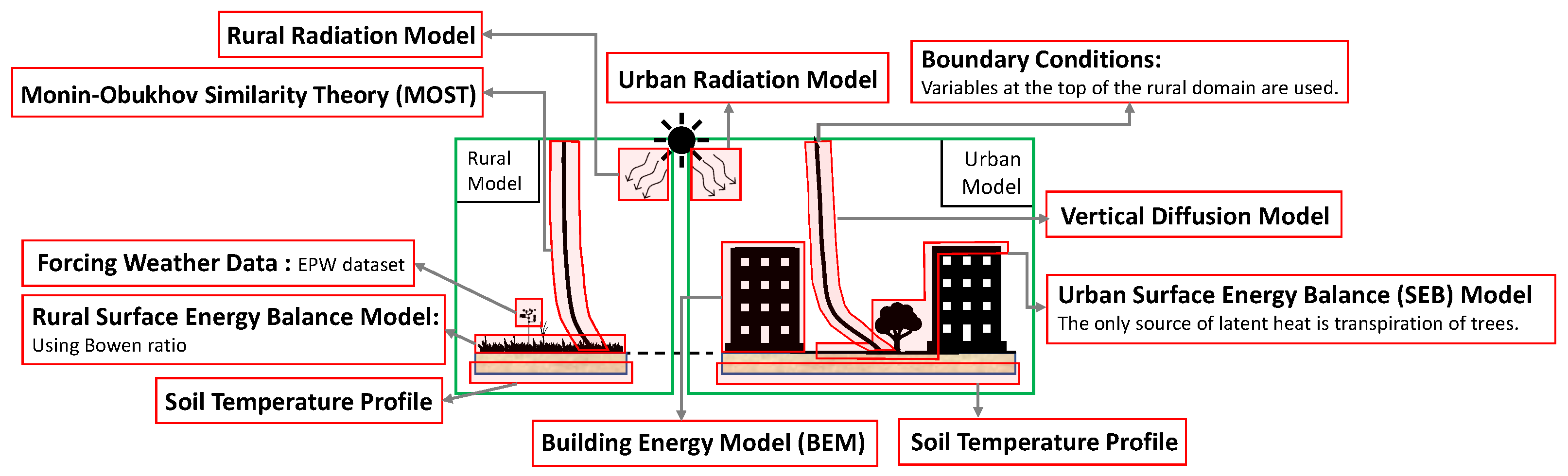
Figure 1, it is composed of several sub-models: a rural model, a one-dimensional urban vertical diffusion model, a radiation model, and a building energy model. VCWG is forced with weather data from a rural site at the vicinity of the urban area. The rural model is used to solve for the vertical profiles of potential temperature, specific humidity, and friction velocity at 10 m a.g.l. The rural model also calculates a horizontal pressure gradient. The rural model outputs are forced on the urban vertical diffusion model that solves vertical transport equations for potential temperature, momentum, specific humidity, and turbulence kinetic energy. This vertical diffusion model is coupled to the radiation and building energy models using two-way interaction. The aerodynamic and thermal effects of urban elements, surface vegetation, and trees are considered. The feedback interaction coupling scheme among the building energy model, radiation model, and the urban one-dimensional vertical diffusion model is designed to update the boundary conditions, surface temperatures, and the source/sink terms in the transport equations in successive time step iterations.
The two-way interaction between the building energy systems and the outdoor environment is determined by the term Q H V A C [W m 2 ] which is the sensible waste heat of the building that is rejected to the outside environment. It is calculated by the building energy model as [39]:
Q H V A C = Q s u r f + Q v e n + Q i n f + Q i n t Q c o o l + W c o o l + Q d e h u m + Q g a s + Q w a t e r ,
Q H V A C = ( Q s u r f + Q v e n + Q i n f + Q i n t Q h e a t ) / η h e a t Q h e a t + Q d e h u m + Q g a s + Q w a t e r ,
under cooling and heating modes, respectively. In these equations all symbols represent positive terms, unless a negative term is emphasized by the negative sign in front of the symbol. Under cooling mode, Q H V A C [W m 2 ] is computed by adding the cooling demand ( Q c o o l [W m 2 ]), consisting of surface cooling demand, ventilation demand, infiltration (or exfiltration) demand, and internal energy demand (lighting, equipment, and occupants), energy consumption of the cooling system ( W c o o l = Q c o o l / C O P [W m 2 ]) (accounting for C O P [-]), dehumidification demand ( Q d e h u m [W m 2 ]), energy consumption by gas combustion (e.g., cooking) ( Q g a s [W m 2 ]), and energy consumption for water heating ( Q w a t e r [W m 2 ]). Under heating mode, Q H V A C [W m 2 ] is computed by adding heating demand ( Q h e a t [W m 2 ]), consisting of surface heating demand, ventilation demand, infiltration (or exfiltration) demand, and internal energy demand (lighting, equipment, and occupants) (divided by thermal efficiency of the heating system ( η h e a t [-])), subtracting the heating demand, adding the dehumidification demand ( Q d e h u m [W m 2 ]), energy consumption by gas combustion (e.g., cooking) ( Q g a s [W m 2 ]), and energy consumption for water heating ( Q w a t e r [W m 2 ]).
In VCWG, the balance equation for indoor convection, conduction, and radiation heat fluxes is applied to all building elements (wall, roof, floor, windows, ceiling, and internal mass) to calculate the indoor air temperature. Then, a sensible heat balance equation, between convective heat fluxes released from indoor surfaces and internal heat gains and sensible heat fluxes from the HVAC system and infiltration (or exfiltration), is solved to obtain the time evolution of indoor temperature as [34,45]:
V ρ C p d T i n d o o r d t = ± Q s u r f ± Q v e n ± Q i n f ± Q i n t ,
where V [m 3 m 2 ] is indoor volume per building footprint area, T i n d o o r [K] is the indoor air temperature, and the heat fluxes on the right hand side are specified in Equations (1) and (2). More details on the parameterization of the terms in Equation (3) can be found in the literature [34,35,36,37,38,39]. In this convention all symbols represent positive terms however, in the equation either positive or negative signs should be used to emphasize if a term contributes to indoor temperature increase or decrease, depending on the operation mode (cooling versus heating) and environmental conditions (indoor, outdoor, and surface temperatures). Similar equations are solved for the calculation of the dehumidification load (for system under cooling mode) and indoor specific humidity; however, since the dehumidification load is usually less than 10% of the cooling load, it is not reported in this study [34,35,36,37,38].
The earlier version of VCWG (v.1.3.2) is fully described in the literature [39], while in the present study its implementation to simulate renewable and alternative energy systems is explored. The newly-developed VCWG v.1.4.4 is forced with meteorological data obtained from the European Centre for Medium-Range Weather Forecasts (ECMWF) ERA5 data product for Guelph, Canada, in 2015 (https://www.ecmwf.int/en/forecasts/datasets/reanalysis-datasets/era5 (accessed 15 March 2021)).

2.2. Guelph Climate and the Urban Fabric

Guelph is a mid-latitude city, with a population of 131,794 and an urban area of 87.22 km 2 , situated in south-western Ontario, Canada, characterized by cold winters and humid summers. The mean daily temperature in Guelph varies from 6.9 °C in January to + 19.7 °C in July (https://en.wikipedia.org/wiki/Guelph (accessed 2 July 2021)). The single-family residential dwellings in south-western Ontario are characterized as one or two-story buildings with varying building planar area densities, vegetation type, and vegetation structure. The urban climate of Guelph and south-western Ontario have been characterized in previous environmental field campaigns [44,46,47]. For instance an Urban Heat Island (UHI) of 0.7 K have been measured in Guelph [46], and the urban meteorological variables, including mean and turbulence statistics, are known to vary according to the street canyon and wind directions, wind speeds, and thermal stability conditions [46,47]. Table 1 shows the input parameters associated with the simulations in residential areas of Guelph. The input parameters are informed by previous studies, including the above. The new model development is described in the following subsections.

2.3. System Integration in VCWG v1.4.4

The active thermal storage is considered as the main paradigm in this study, supplemented by other building renewable energy systems. 
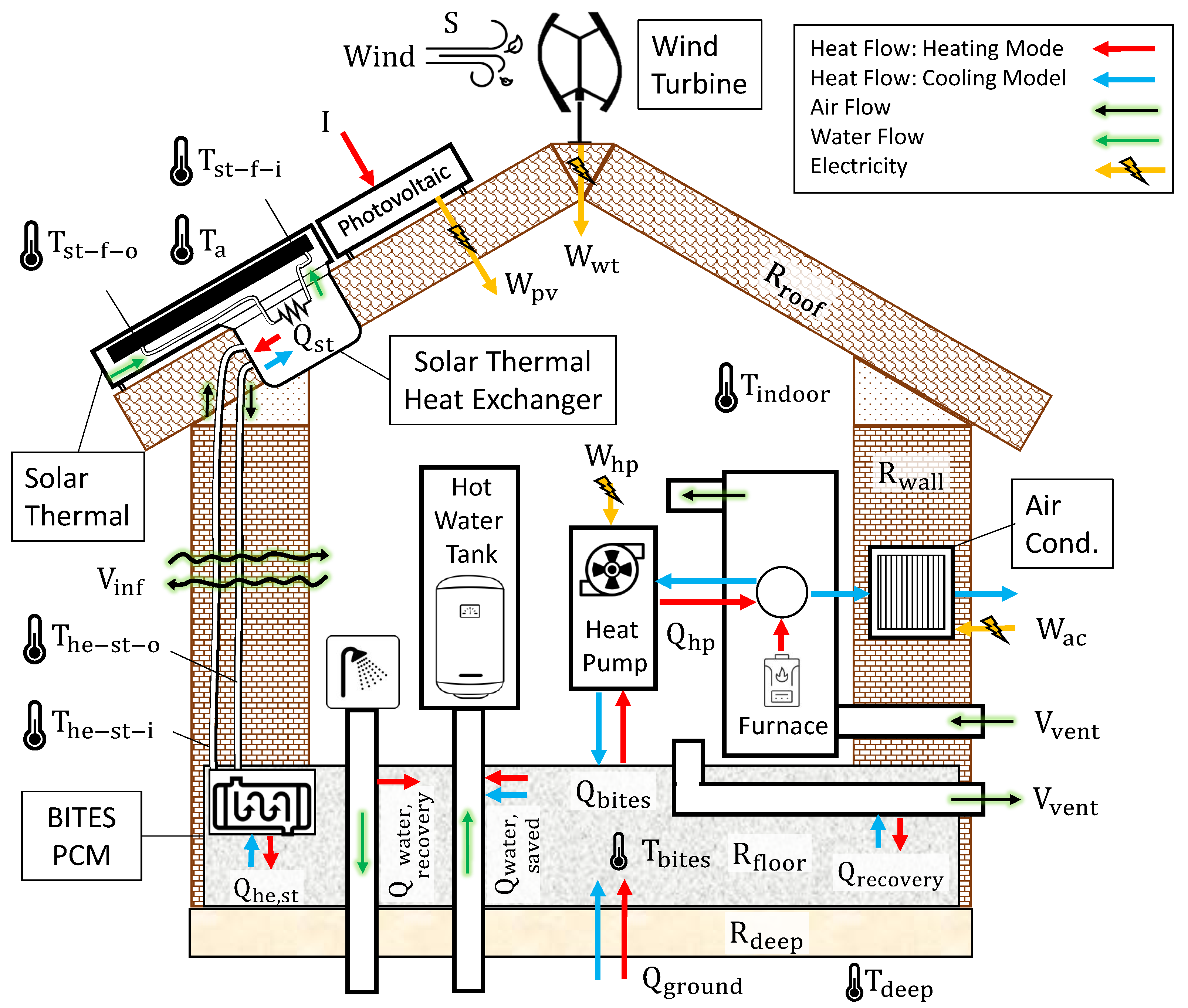
Figure 2 shows the building systems via integration of Solar Thermal (ST), PhotoVoltaic (PV), Wind Turbine (WT), Building Integrated Thermal Energy Storage (BITES) system, Phase Change Material (PCM), Heat Pump (HP), and heat recovery systems as well as the utilization of ground thermal energy. The space heating and cooling can be supplemented via a HP. In this configuration, the BITES system is charged or discharged using the ST collector, HP, exhaust air, supply water, or grey water. Concrete is considered due to its common use in building structures and convenience of heat transfer optimization via embedded pipe design with liquid or air as heat transfer fluids [12,25]. The BITES system acts as either a cold (under heating mode) or warm (under cooling mode) reservoir of heat for the HP system. Energy recovery can be considered via the exhausted ventilation air. Another heat recovery system allows ejection of thermal energy from used domestic (grey) water into the BITES system under the heating mode. The system is equipped with a WT. PCM technology is considered to modulate the BITES temperature if temperatures are favorable, supported by successful evidence of using PCM with concrete for thermal storage [16]. Water heating can be achieved using the BITES system if its temperature is greater than the water temperature to be heated. Ground thermal energy in the form of heat flux can be exchanged between the deep soil and the BITES system. This flux could be either desirable or undesirable for a given season and system configuration. Table 2 shows the system design parameters.
The control design for thermally-activated buildings is very important via the setting of temperatures, mass flow rates, and operation of various building systems [10]. 
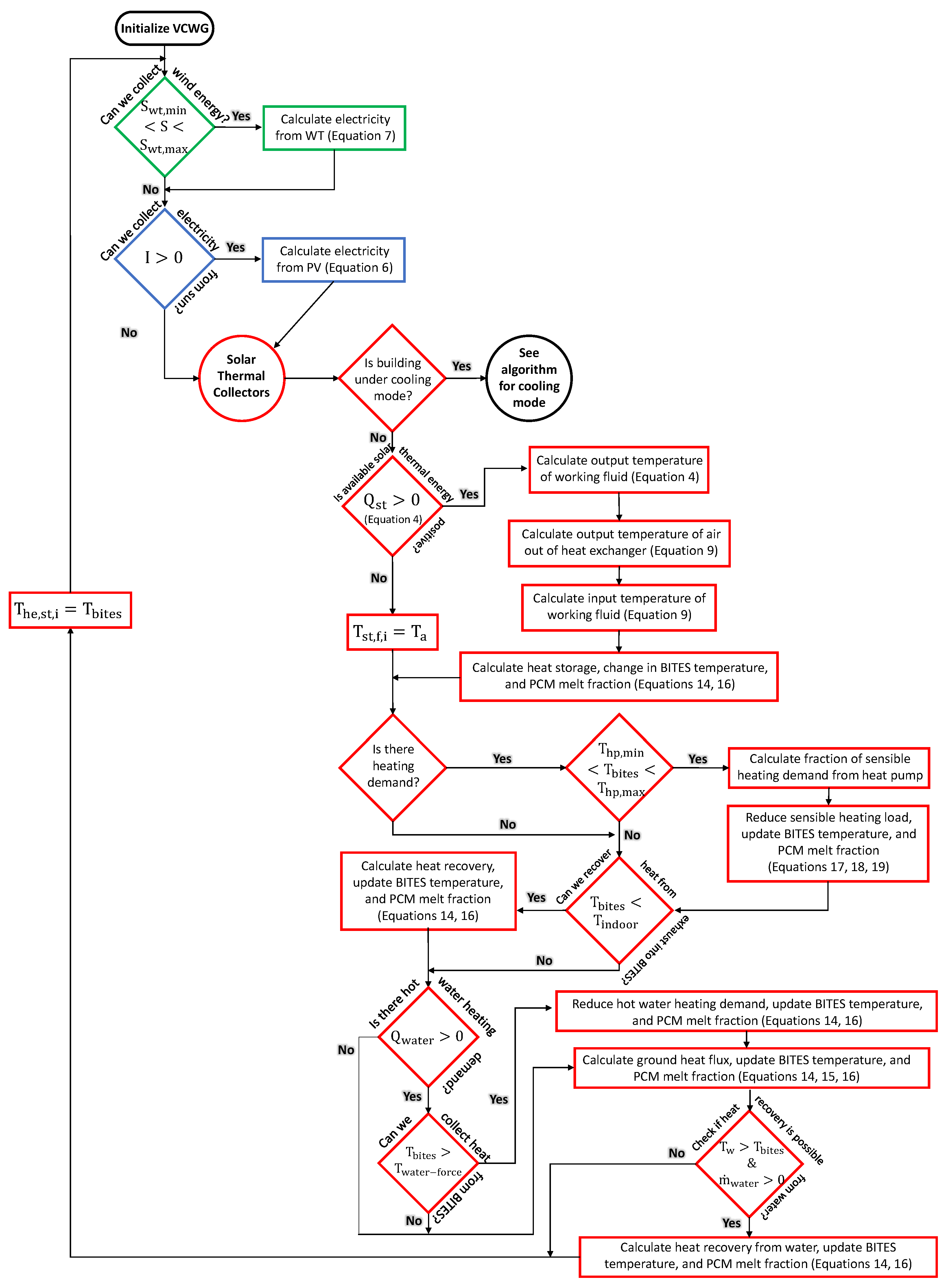
Figure 3 shows the control algorithm for the system under heating mode. The ST collector attempts to heat the BITES system and raise its temperature when solar thermal energy is available. If BITES is to be used as a heat source for the HP, then the BITES temperature determines the C O P h p of HP. Furthermore, the fraction of the sensible heating demand to be supplied by the HP is determined using this temperature-dependent C O P h p 
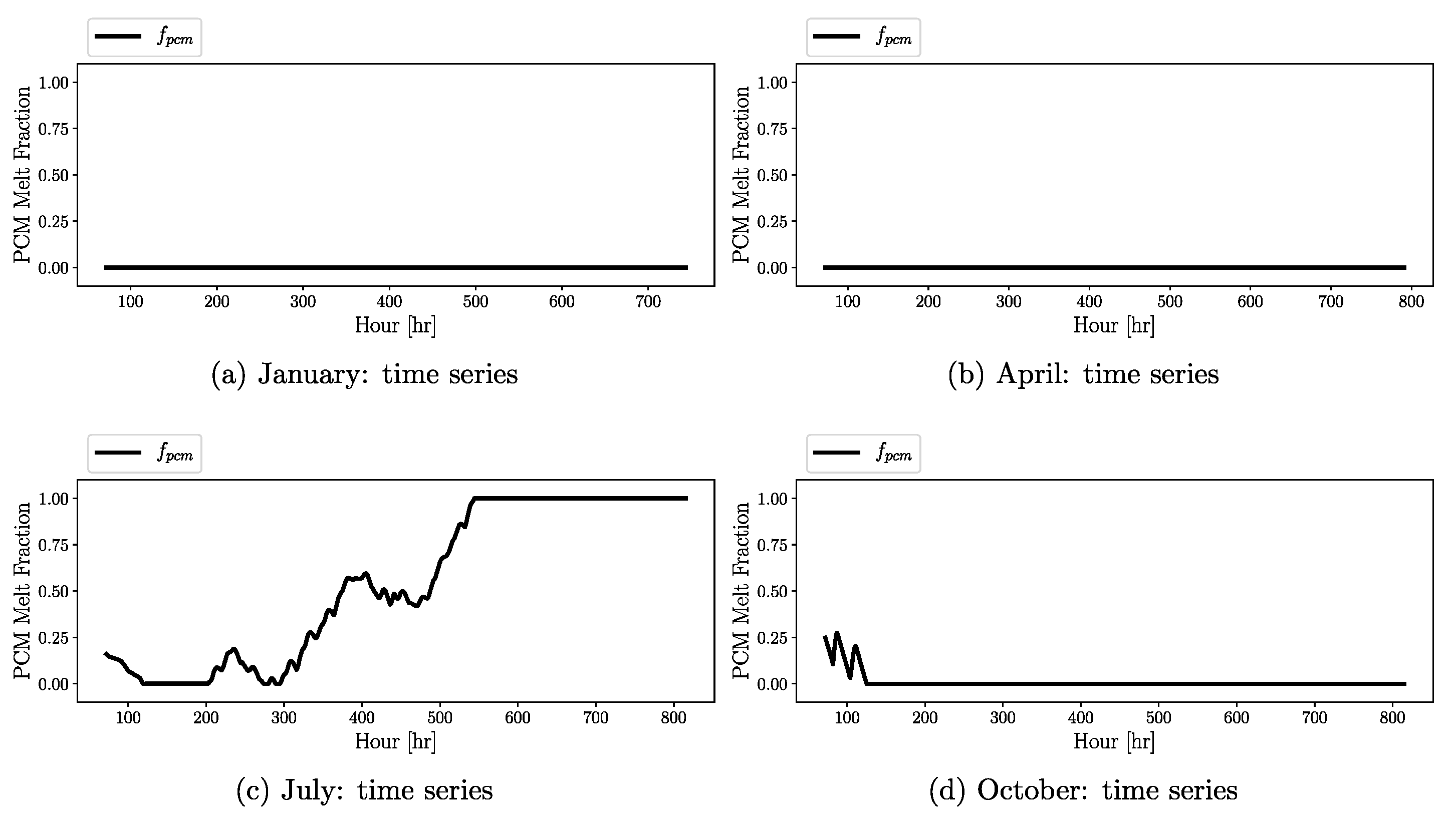
. The BITES system is not permitted to reach a temperature below the minimum temperature required for the HP to operate. If this occurs, or if any fraction of heat is not to be supplied by the HP, then the required heating demand is supplied by the standard heating furnace that relies on natural gas. Heat recovery from the exhausted ventilated air is possible if the exit indoor air temperature is greater than the BITES temperature. A key variable to track is the fraction of the PCM that is melted. If this fraction is between 0 and 1, the heat exchanged with the PCM occurs by either melting the PCM (adding heat to BITES) or solidifying PCM (extracting heat from BITES) while keeping the BITES temperature the same. If the fraction of melted PCM reaches 0, there is no more solidification possible, where the removed heat will contribute to lowering the BITES temperature by sensible cooling. Likewise, if the fraction of the melted PCM reaches 1, there is no more melting possible, where the added heat will contribute to increasing the BITES temperature by sensible heating. The amount of heat used from BITES for water heating is determined by the building water usage schedule and the water inlet temperature. The BITES system can only warm up the water to its current temperature, while any further heating of the water must be achieved by auxiliary natural gas combustion in the hot water tank. Heat recovery by used domestic water is achieved if waste water temperature is greater than the BITES temperature. The ground heat flux is computed and its effect on BITES temperature or PCM melt fraction is accounted for.
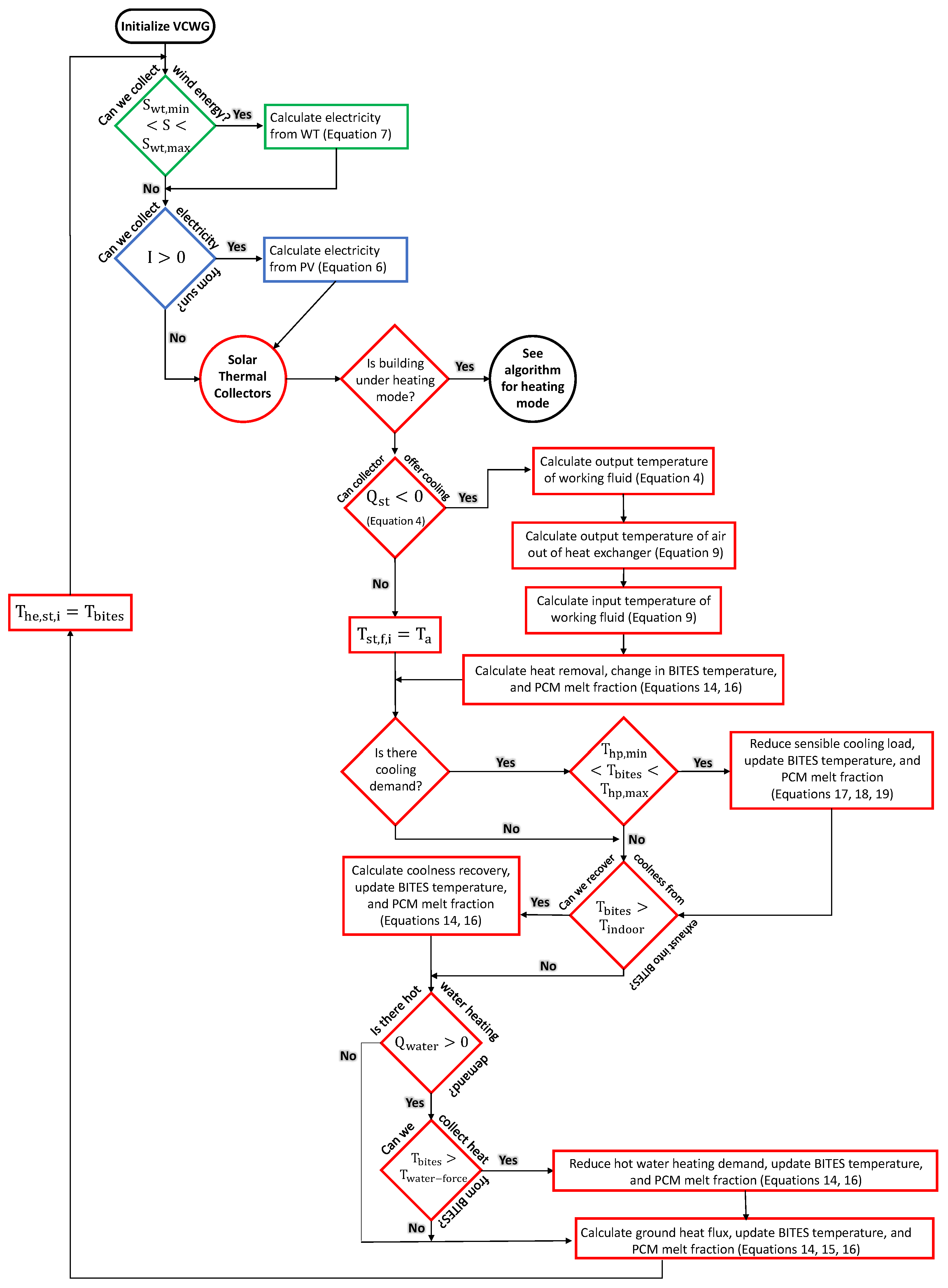
Figure 4 shows the control algorithm for the system under cooling mode. The ST collector attempts to cool the BITES system and lower its temperature when thermal energy can be lost via the collector. If BITES is to be used as a heat sink for the HP, then the BITES temperature determines the C O P h p for the HP. Furthermore, the entire amount of sensible cooling demand is set to be met by the HP using this temperature-dependent coefficient of performance. The BITES system is not permitted to reach a temperature above the maximum temperature required for the HP to operate. If this occurs, the standard air conditioning unit is operated. Heat recovery from the exhaust ventilated air is possible if the exit indoor air temperature is less than the BITES temperature. The same logic holds for utilizing PCM and water heating under the cooling mode as in the heating mode. There is no heat recovery from used domestic water under cooling mode. The ground heat flux is computed and its effect on BITES temperature or PCM melt fraction is accounted for.

2.3.1. Solar Thermal Collectors

The Hottel–Whillier–Bliss model is commonly used for the design and analysis of free-standing (i.e., not building integrated) flat plate solar thermal collectors [48]. This model considers an energy balance consisting of shortwave radiation gain, longwave radiation loss, and convective loss to air at ambient conditions to determine the available solar energy Q s t [W m 2 ] for a flat plate collector [48]:
Q s t = F R s t A s t ( τ α ) e I U s t ( T s t , f , i T a ) = m ˙ s t , f c s t , f ( T s t , f , o T s t , f , i ) ,
where F R s t [-] is the heat removal factor, A s t [m 2 m 2 ] is the collector area per building footprint area, ( τ α ) e [-] is the effective transmittance-apsorptance product, I [W m 2 ] is the incident shortwave radiation flux normal to the collector, U s t [W m 2 K 1 ] is the convective and radiative heat loss coefficient, T s t , f , i [K] is the inlet fluid temperature to the collector, T s t , f , o [K] is the outlet fluid temperature from the collector, T a [K] is the ambient atmospheric temperature, m ˙ s t , f [kg s 1 m 2 ] is the mass flow rate of the fluid through the collector per unit building footprint area, and c s t , f [J kg 1 K 1 ] is the heat capacity of the fluid at constant pressure.
If the collector tilt angle is β s t [ ], the zenith angle is θ z , the azimuth angle is θ a [ ], the direct shortwave radiation flux vector from the sky is S d i r [W m 2 ], and the diffuse shortwave radiation flux vector from the sky is S d i f f [W m 2 ], the incident shortwave radiation flux normal to the collector I [W m 2 ] is [49]:
I = S d i r cos θ a cos ( θ z β s t ) + S d i f f .

2.3.2. Photovoltaic Collectors

It is true that the conversion efficiency of a solar photovoltaic cell depends modestly on ambient temperature. However, in practical modeling, a constant conversion efficiency can be considered. The electricity power conversion of a photovoltaic system per building footprint area can be calculated as [49]:
W p v = η p v A p v I = η p v A p v S d i r cos θ a cos ( θ z β p v ) ,
where A p v [m 2 m 2 ] is the collector area per building footprint area, η p v [-] is conversion efficiency, and β p v [ ] is the tilt angle of the photovoltaic system.

2.3.3. Wind Turbines

The most generic wind turbine equation for electricity production W w t per building footprint area is employed and valid when wind speed is within a specified operational range of minimum and maximum possible wind speeds. The equation is given as [50]:
W w t = 0.5 η w t ρ A w t S 3 ,
where η w t [-] is the turbine efficiency, ρ [kg m 3 ] is the air density, and S [m s 1 ] is the wind speed near the roof level of a building, and A w t [m 2 m 2 ] is the swept area of the turbine per building footprint area [50].

2.3.4. Heat Exchangers

A typical heat exchanger that is used in building energy systems is the counter-flow heat exchanger. In the present model, such a heat exchanger is needed to transfer the thermal energy between the working fluid of the solar thermal collector and the air stream that is circulating through the BITES system. The objective of a simplistic model for a heat exchanger is to find a relationship between inlet and outlet temperatures for the two streams of the fluids. This relationship can be given using the efficiency of the heat exchanger:
η h e , s t = T s t f o T s t f i T s t f o T h e s t i .
From the energy balance of a heat exchanger and knowing the efficiency of a heat exchanger, it is possible to arrive at an equation for T h e s t o [K] given other inlet temperatures ( T s t f o and T h e s t i [K]), mass flow rates ( m ˙ s t , f and m ˙ h e , s t [kg s 1 m 2 ]), and heat capacities ( c s t , f and c a i r [J kg 1 K 1 ]):
T h e s t o T h e s t i = m ˙ s t , f c s t , f m ˙ h e , s t c a i r ( T s t f o T s t f i ) = m ˙ s t , f c s t , f m ˙ h e , s t c a i r η h e , s t ( T s t f o T h e s t i ) T h e s t o = m ˙ s t , f c s t , f m ˙ h e , s t c a i r η h e , s t ( T s t f o T h e s t i ) + T h e s t i .

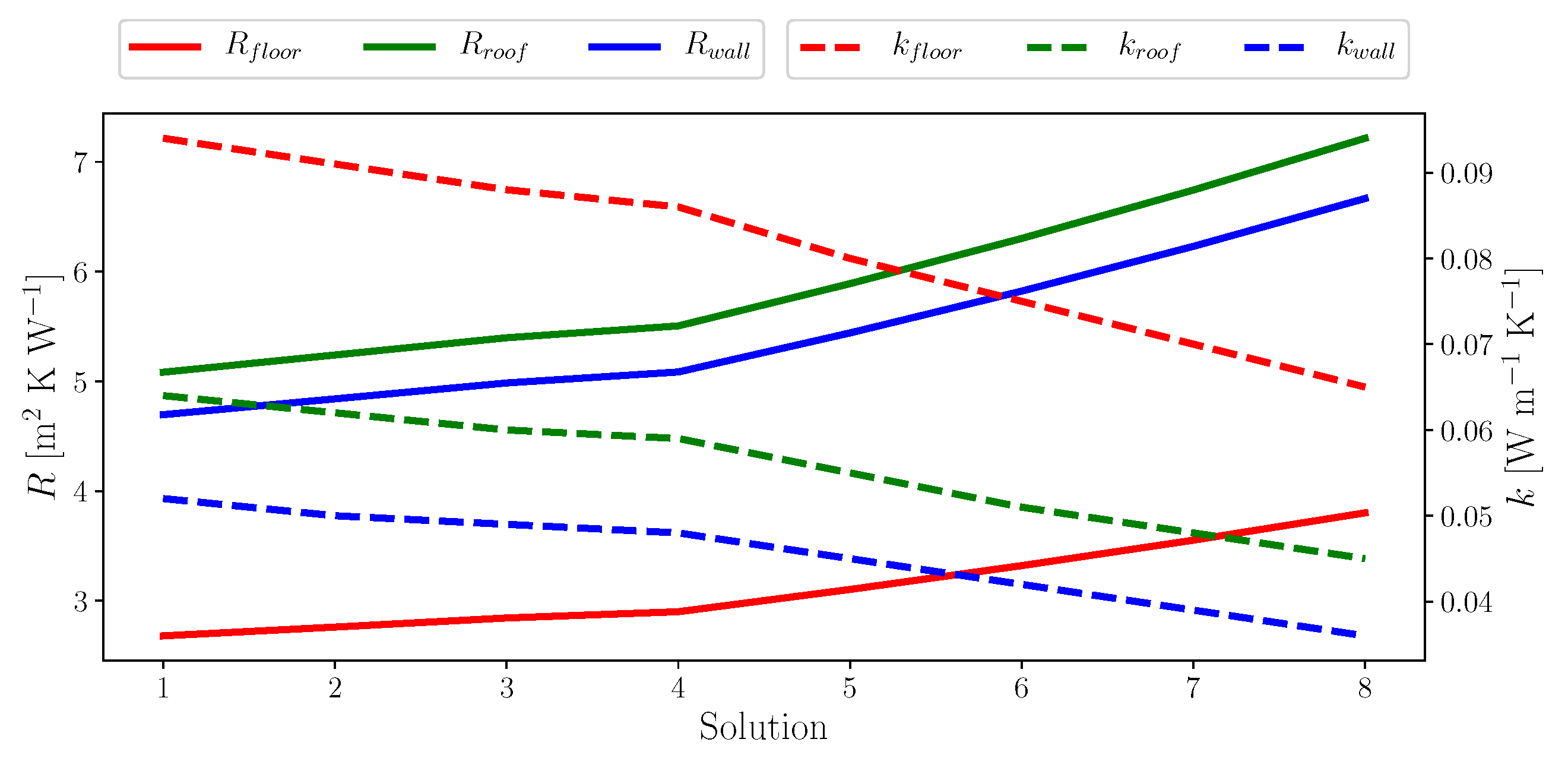
2.3.5. Building Envelop

The resistance value of a building construction material is calculated by dividing the construction material thickness Δ x [m] by the thermal conductivity k [W m 1 K 1 ]:
R = Δ x k .
For a multi-layer construction material, the total resistance value is computed by adding the individual resistances:
R t o t = R 1 + R 2 + R n = Δ x 1 k 1 + Δ x 2 k 2 + Δ x n k n .
By the same approach the total conductivity can be calculated as:
k t o t = Δ x t o t R t o t .
The volumetric heat capacity for the total envelop of interest (e.g., wall, roof, or floor) can be computed by weighted averaging using the layer thicknesses:
c v = Δ x 1 ρ 1 c p 1 + Δ x 2 ρ 2 c p 2 + + Δ x n ρ n c p n Δ x t o t .
Table 3 shows the details of the construction layers for external walls, roof, and floor that are associated with a high-performance building envelop based on Expanded PolyPropylene (EPP). The total volumetric heat capacity for the external walls, roof, and floor are computed as c v , w a l l = 289,010.9, c v , r o o f = 195,080, and c v , f l o o r = 1,258,814 [J m 3 K 1 ], respectively.

2.3.6. Thermal Energy Storage

A simple way to model thermal energy storage is to ignore PCMs and to consider a lump system with uniform temperature T b i t e s [K] throughout the BITES system. With these assumptions, using energy balance, the change in temperature of a BITES system over finite time Δ t [s], subject to heat gains Q g a i n , i [W m 2 ], heat losses Q l o s s , i [W m 2 ], and ground heat transfer Q g r o u n d [W m 2 ] can be written as:
Δ T b i t e s V b i t e s c b i t e s = + i = 1 n Q g a i n , i Δ t i = 1 m Q l o s s , i Δ t + Q g r o u n d Δ t ,
where Δ T b i t e s [K] is a change in the temperature of the BITES system, V b i t e s [m 3 m 2 ] is the volume of the BITES system per unit building footprint area, and c b i t e s [J m 3 K 1 ] is the volumetric heat capacity of the BITES system. It is interesting to note that the BITES system can be thermally charged or discharged using multiple sources and sinks of energy, so the gains and losses are shown using a summation notation. The availability of heat gains and losses are strongly dependent on temperatures of the surrounding systems that the BITES is interacting with. A source of energy for the BITES system (e.g., solar thermal system) should be at a higher temperature, while a sink of energy for the BITES system (e.g., ground) should be at a lower temperature.
The ground heat flux is computed by having a resistance R d e e p [m 2 K W 1 ] between the BITES temperature T b i t e s [K] and the deep soil temperature T d e e p [K]. This heat flux could act as a source (warming BITES) or sink (cooling BITES) of thermal energy for the BITES. The ground heat flux can be calculated as:
Q g r o u n d = T d e e p T b i t e s R d e e p .
When PCMs are used, the net heat transfer to the material results in either melting or solidifying a portion of the volume of the material without changing the temperature of the thermal storage system. This can be given by:
Δ V p c m l p c m = i = 1 n Q g a i n , i Δ t i = 1 m Q l o s s , i Δ t + Q g r o u n d Δ t ,
where Δ V p c m [m 3 m 2 ] is the change in volume of PCM melted (positive) or solidified (negative) per unit building footprint area and l p c m [J m 3 ] is the volumetric latent heat of melting/solidification.

2.3.7. Heat Pumps

The first law of thermodynamics can be expressed for the HP, which states that the electricity consumption ( W h p ) plus the heat removed from a cold reservoir of heat ( Q L ) should be equal to the heat forced into a warm reservoir of heat ( Q H ). Furthermore, the C O P h p for the HP is defined differently under heating or cooling modes. The following three equations are relevant [21]:
W h p + Q L = Q H ,
C O P h p = Q H W h p ( Heating mode ) ,
C O P h p = Q L W h p ( Cooling mode ) .

2.4. Economic Assessment

Economic analysis is an essential part of system optimization since cost is usually an important objective function. The European Committee for Standardization (CEN), offers the standard prEN 15459-1 (economic evaluation procedure for energy systems in buildings), which provides the Global Cost method for assessment of relative economic feasibility of multiple building energy configurations with respect to one another [2,51]. This method considers all costs associated with a building energy configuration, including initial investment cost, operation and maintenance cost, fuel cost, and more. It also accounts for a discount rate over an investment period of usually N = 30 years. This method can calculate three alternative cost metrics: (1) present value of the global cost, which moves all costs in time to the present time; (2) annualized cost, which distributes all costs to an equal annual value; and (3) pay-back period, which provides the number of years in which the marginal initial cost of a building configuration system will be balanced by the accumulation of annual savings. All three metrics are useful, but in this study we mainly report the annualized cost, as the primary metric, given by:
C A = C I + C G + C E + C O M C S ,
where C I is the annualized initial investment for system installation and commissioning, C G is the annualized cost of gas consumption, C E is the annualized cost of electricity consumption, C O M is the annualized cost of operation and maintenance, and C S is the annualized revenue of discarding the system, which has a salvage value. All costs in this equation are per unit building footprint area [$ m 2 ].
In the present analysis, it is important to know the marginal annualized cost, which is the difference in cost of a system retrofitted with renewable energy and a pre-existing system, on top of which the renewable energy systems are added. In other words, since the building is not completely net-zero, it still requires a standard water heater, furnace, air conditioner, etc. From here forward, any cost computed will correspond to this marginal annualized cost.
Without any renewable energy, the marginal initial cost for a conventional system is C B [$ m 2 ]. This cost is non-zero since without renewable energy, the conventional system should be over-sized to meet the energy demand of the building. This annualized cost can be given by [49]:
C I B = C B × C R F ( i , N ) .
The capital recovery factor computes the annual payment required to form a total present worth of an amount given an effective interest rate i and the number of years N. The capital recovery factor and effective interest rate are given by [49]:
C R F ( i , N ) = i 1 ( 1 + i ) N ,
i = i n j 1 + j ,
where i n is the nominal interest rate and j is the inflation rate.
The annualized initial investment for renewable energy systems can be computed by adding the price of equipment, subtracting the government rebate (or incentive) for retrofitting the house with renewable energy, and annualizing the cost using the capital recovery factor:
C I = [ A p v P p v + A w t P w t + A s t P s t + V b i t e s P b i t e s + V p c m P p c m + P h p + P e n v R ] × C R F ( i , N ) ,
where P k represents the unit installation cost for a given system and R represents the unit rebate value. For PV collectors, P p v [$ m 2 ] is provided per unit collector area; for WT, P w t [$ m 2 ] is provided per unit swept area of wind; for ST, collectors P s t [$ m 2 ] is provided per unit collector area; for BITES, P b i t e s [$ m 3 ] is provided per unit volume; for PCM, P p c m [$ m 3 ] is provided per unit volume; for HP, P h p [$ m 2 ] is provided per unit building footprint area; for the building envelop P e n v , [$ m 2 ] is provided per unit building footprint area; and for the rebate R, [$ m 2 ] is provided per unit building footprint area.
The annualized cost of gas consumption, for both the base energy system and the system using renewable energy, should be computed by considering the annual rate of increase in gas price j G and the present worth factor P W F ( i , k ) , given by [49]:
C G B = C G = k = 1 N ( G h + G w h ) × P G × ( 1 + j G ) k × P W F ( i , k ) C R F ( i , N ) ,
P W F ( i , k ) = 1 ( 1 + i ) k ,
where G h and G w h [m 3 m 2 ] are total annual gas consumption per building footprint area required for space and water heating, respectively, and P G [$ m 3 ] is the current gas price per cubic meter at standard pressure.
The annualized cost of electricity consumption for the base energy system should be computed by considering the annual rate of increase in electricity price j E :
C E B = k = 1 N ( E c + E d ) × P E × ( 1 + j E ) k × P W F ( i , k ) C R F ( i , N ) ,
where E c and E d [kW hr m 2 ] are total annual electricity consumption per building footprint area required for space cooling and domestic use, respectively, and P E [$ kW 1 hr 1 ] is the current electricity price.
The annualized cost of electricity consumption for the renewable energy system should consider more terms that relate to electricity required for heating by the HP E h [kW hr m 2 ] and electricity generated by the PV collector E p v [kW hr m 2 ] and WT E w t [kW hr m 2 ] such that:
C E = k = 1 N ( E h + E c + E d E p v E w t ) × P E × ( 1 + j E ) k × P W F ( i , k ) C R F ( i , N ) .
The annualized marginal cost of operation and maintenance for the base system may be assumed to equal to C O M B = 5 $ m 2 , which would be lower than the same cost for the renewable energy system, given by:
C O M = A p v O M p v + A w t O M w t + A s t O M s t + V b i t e s O M b i t e s + V p c m O M p c m + O M h p ,
where O M p v [$ m 2 ] is the operation and maintenance cost for the PV collector per unit collector area; O M w t [$ m 2 ] is the cost for WT per unit swept area of wind; O M s t [$ m 2 ] is the cost for the ST collector per unit collector area; O M b i t e s [$ m 3 ] is the cost for BITES per unit volume; O M p c m [$ m 3 ] is the cost for PCM per unit volume; and O M h p [$ m 2 ] is the cost for HP per unit building footprint area.
The annualized revenue of discarding the system, which has a salvage value, can be computed by assuming a salvage factor, F S B or F S for the base and renewable energy systems, respectively, and applying the P W F ( i , N ) and C R F ( i , N ) for the full period of N years:
C S B = F S B × C I B × P W F ( i , N ) × C R F ( i , N ) ,
C S = F S × C I × P W F ( i , N ) × C R F ( i , N ) .
The payback period can be calculated by equating the present worth of the difference in annual cost of running the systems (base minus renewable energy) to the difference in the initial cost of the systems (renewable energy minus the base) [51]:
k = 1 N p a y b a c k C k × P W F ( i , k ) C I C I B ,
where C k [$ m 2 ] is the difference in the annual cost of running the systems (base minus renewable energy). At N p a y b a c k , this equality is satisfied.
Table 4 shows the parameters chosen for economic analysis. Note that the nominal interest rate i n is taken as the estimated variable mortgage rate in 2021 from the Bank of Canada based on the rationale that the renewable energy investment is likely financed using a house mortgage (https://www.bankofcanada.ca/rates/interest-rates/ (accessed 13 April 2021)). The inflation rate is retrieved from the Bank of Canada by comparing the cost of a basket of goods and services from 2020 to 2021 (https://www.bankofcanada.ca/rates/related/inflation-calculator/ (accessed 13 April 2021)). The price of natural gas is retrieved for 2021 from the Ontario Energy Board (OEB) (https://www.oeb.ca/rates-and-your-bill/natural-gas-rates (accessed 13 April 2021)). The projected annual increase for the price of natural gas is taken from the Government of Ontario (https://www.ontario.ca/document/fuels-technical-report/module-4-fuels-system-cost-outlook (accessed 13 April 2021)). The price of electricity is retrieved for 2021 from the Ontario Energy Board (OEB) (https://www.oeb.ca/rates-and-your-bill/electricity-rates (accessed 13 April 2021)). The annual increase for the price of electricity in the future is estimated by the historical records during the last 10 years from the Ontario Energy Board (OEB) https://www.oeb.ca/rates-and-your-bill/electricity-rates/historical-electricity-rates (accessed 13 April 2021) and the Canada Energy Regulator (CER) (https://www.cer-rec.gc.ca/en/data-analysis/energy-markets/market-snapshots/2017/market-snapshot-canadian -electricity-prices-generally-increasing-faster-than-inflation-but-trends-vary-among-provinces.html (accessed 16 April 2021)).
The initial price of an ST collector is retrieved from a Canadian supplier (Latitute 51 Solar 30-Tube Solar Collector) (https://www.latitude51solar.ca/30-tube-solar-collector (accessed 13 April 2021)). The initial price of a PV collector is retrieved from EnergySage LLC (https://www.energysage.com/local-data/solar-panel-cost/ca/san-bernardino-county/ontario/ (accessed 13 April 2021)) and the Canada Energy Regulator (CER) (https://www.cer-rec.gc.ca/en/data-analysis/energy-commodities/electricity/report/solar-power-economics/economics -solar-power-in-canada-appendix-methods.html (accessed 16 April 2021)), factoring in the Federal Investment Tax Credit (ITC) and other local solar incentives in Ontario [52]. The initial price of a WT is retrieved from a Canadian supplier (Sunforce 30 ft. Wind Generator Tower Kit). (https://sunforceproducts.com/products/30-ft-wind-generator-tower-kit/ (accessed 13 April 2021)). The initial price of a HP is retrieved from a Canadian supplier (Senville 24000 BTU Mini Split Air Conditioner—Heat Pump—SENL/24CD) (https://senville.ca/24000-btu-mini-split-air-conditioner-senl-24cd/ (accessed 14 April 2021)). The initial price of PCM is retrieved from an American supplier (Jedwards International, Inc. Paraffin Wax https://bulknaturaloils.com/paraffin-wax-fully-refined.html (accessed 14 April 2021)). The initial price of BITES is retrieved from a Canadian supplier (Canada Building Materials Ready Mix Concrete at 25 MPa Strength) (http://www.canadabuildingmaterials.com/ (accessed 14 April 2021)). Some systems may require a replacement over the investment horizon. These are the WT, PCM, and HP. To simplify the economic analysis, it can be assumed that the replacement systems are purchased at the beginning of the investment period, so essentially the initial cost for those systems are twice the cost for a single system.
The initial price of a high performance building envelop can be calculated by considering the unit price of Expanded PolyPropylene (EPP) and dimensions of the house. Consider the house footprint to be 200 m 2 with horizontal dimensions of 10 m × 20 m and a height of 6 m. This requires, approximately, 360 m 2 of walls, 200 m 2 of floor, and 200 m 2 of roof areas. The installation cost of a single layer EPP panel shown in Table 3, including assembly and labor, is P E P P = 29.25 $ m 2 . Usually the walls require two layers of EPP, while the floor and roof require only a single layer of EPP. Given these assumptions, the cost of EPP per unit building footprint area [$ m 2 ] can be calculated as:
P e n v = P E P P ( 2 A b u i l d i n g + 2 A w a l l ) A b u i l d i n g = 29.25 ( 2 × 200 + 2 × 360 ) 200 = 164 .
Various government rebates and incentives exist in Canada to assist home owners to improve the energy efficiency of their homes. For instance The Ontario Renovates Program provides up to $25,000 in forgivable loan assistance to low- and moderate-income households to assist them in upgrading the energy efficiency of their homes (https://dnssab.ca/housing-services/programs/ontario-renovates-program/ (accessed 14 April 2021)). The Enbridge Home Efficiency Rebate provides up to $5000 for home energy upgrades, including insulation, air sealing, window replacement, heating and cooling, hot water, and more (https://windfallcentre.ca/energy/incentives/ (accessed 14 April 2021)). The Enbridge Home Winter Proofing Insulation rebate offers $500 for improving the thermal insulation of homes in critical areas (https://www.hometradestandards.com/rebates (accessed 14 April 2021)). The Union Gas Home Reno Rebate offers $5000 for switching to two or more energy-efficient HVAC units (https://www.hometradestandards.com/rebates (accessed 14 April 2021)). The Grey water Reuse System program at the City of Guelph provides a credit of $1000 for systems that collect and use grey water from household showers and baths (https://showmethegreen.ca/ (accessed 14 April 2021) ). These rebates can be assumed to apply to the economic analysis for a total rebate value of $36,500. Assuming the footprint of a two-storey house to be 200 m 2 , the rebate value per unit building footprint area is R = 182.5 $ m 2 .
The operation and maintenance cost of each renewable energy system can be scaled using the initial system cost [2]. Some systems are known to require higher operation and maintenance costs, such as the HP and WT, while other systems impose lower costs. The salvage factor for the base system can be assumed to be lower than the renewable energy system.

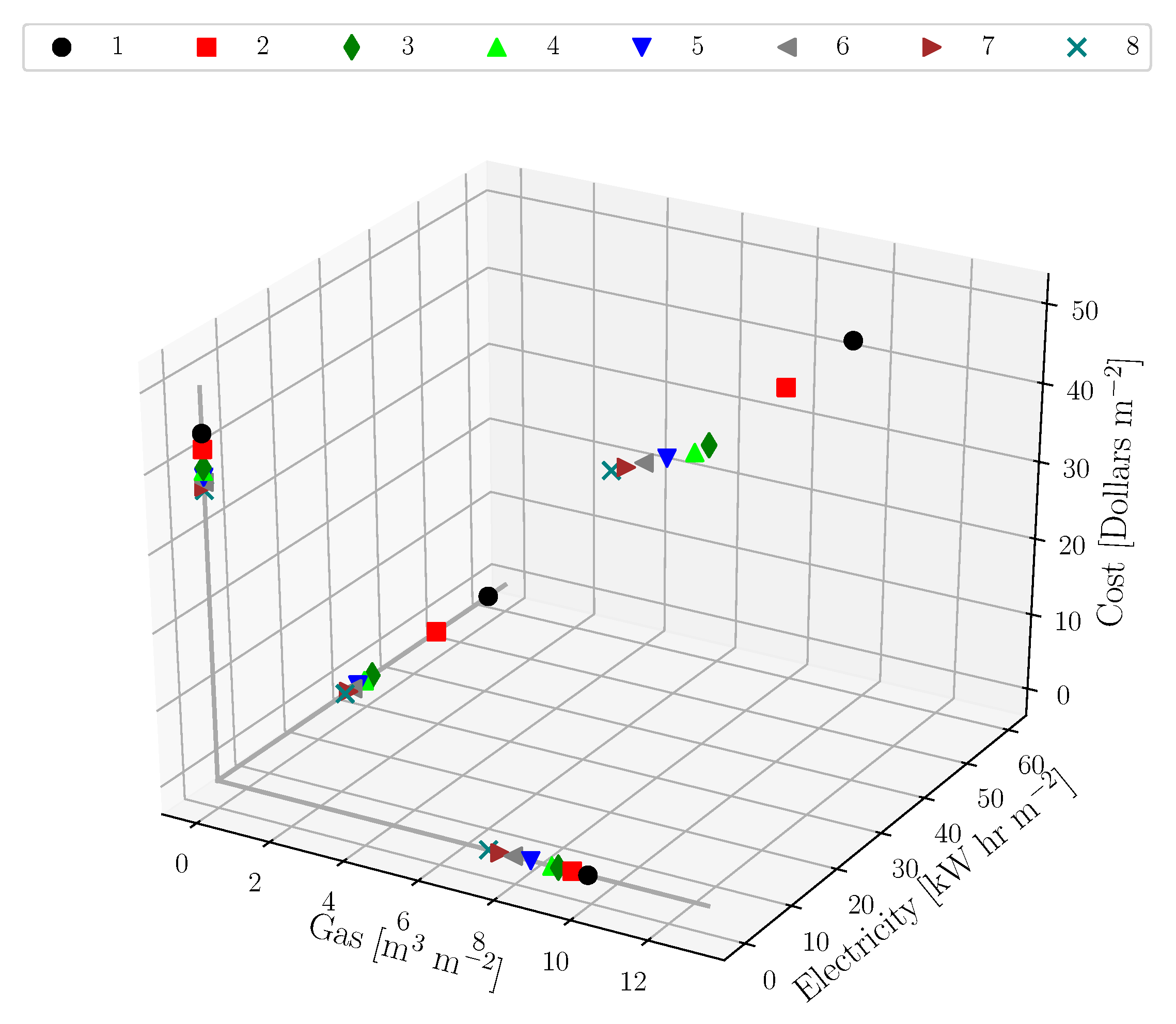
2.5. System Optimization

A key optimization problem arises when sizing the components of the renewable energy system. On the one hand, sizing up a component of the system would likely result in greater energy savings and possibly fuel costs; on the other hand, however, the energy savings may impose a greater price premium due to larger capital investment, operation, and maintenance required.
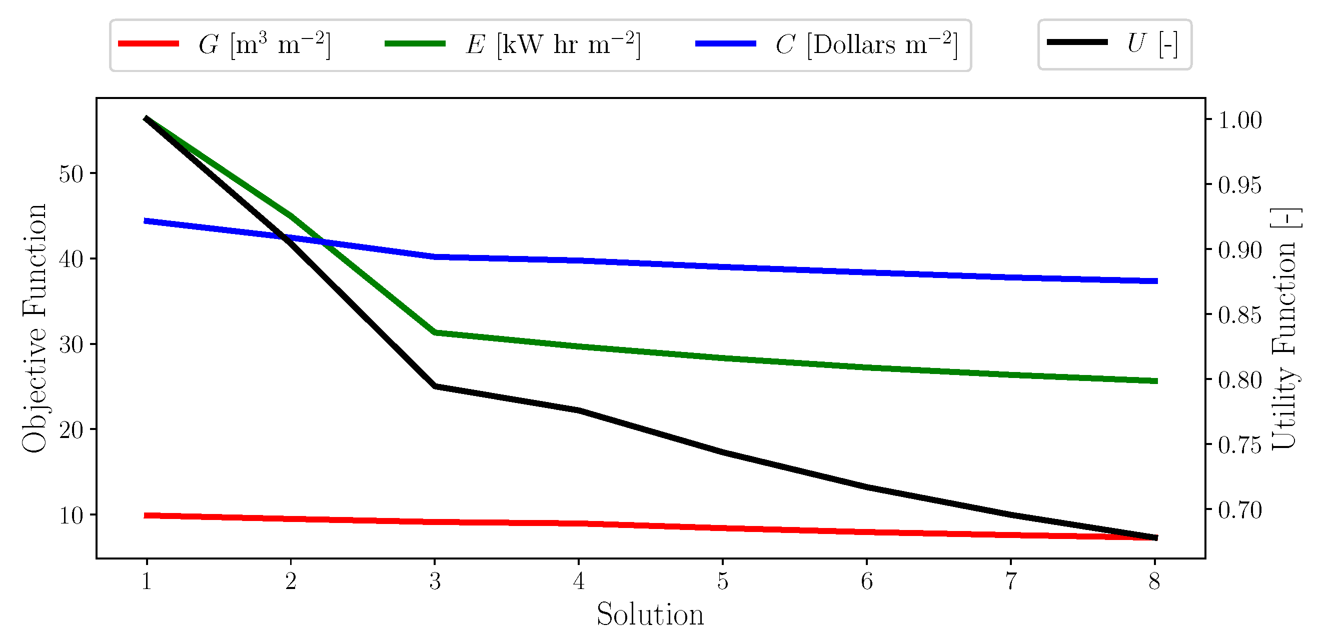
The weighted-sum approach is a common technique for multi-objective optimization [53]. In our case, the multi-objective function to be minimized is given by the utility function as [53]:
U ( x ) = w G G ( x ) + w E E ( x ) + w C C ( x ) ,
where G ( x ) , E ( x ) , and C ( x ) are the gas consumption [m 3 m 2 ], electricity consumption [kW hr m 2 ], and cost [$ m 2 ] objective functions, respectively; and w G , w E , w C are the corresponding weights. Here x = [ x 1 , x 2 , , x 8 ] 
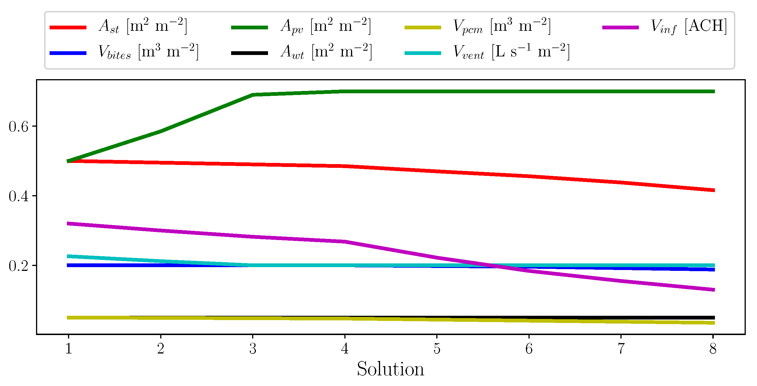
is the vector of design parameters that is subject to constraints x i , m i n x i x i , m a x . The design parameters of choice are x 1 = A s t , x 2 = V b i t e s , x 3 = A p v , x 4 = A w t , x 5 = V p c m , x 6 = V v e n t , x 7 = V i n f , and x 8 , which is the combination of wall-roof-floor thermal resistances (conductivities). Note that x 8 is defined as a combined parameter so that all resistances (conductivities) would change by the same percentage.
The utility function minimum is dependent on the choice of the set of weights, and for a given set, the solution to the optimization problem is pareto optimal. On a pareto front, the optimization has been reached, i.e., the utility function has been minimized, at least locally, and moving on this front may improve (reduce) one objective function while degrading (increasing) another objective function [53]. One common problem is the choice of the weights, since there is usually arbitrariness in the choice given the user (or decision maker) preferences to weigh some objective functions higher than the others. However, it is recommended that the weights (1) be all positive, (2) usually consider the magnitude of each objective function, and (3) be ranked according to a well-established method to prefer some objectives over the others. Although there is no strict requirement, it is recommended that i n w i = 1 [53].
One way to consider the magnitude of each objective function is to normalize it by its maximum possible value. In our case, the maximum values for G ( x ) , E ( x ) , and C ( x ) are not trivial, so alternatively the objective functions can be normalized by the starting value of the initial solution to the optimization, i.e., the utility function can be written as:
U ^ ( x ) = w G G ( x ^ ) G 1 + w E E ( x ^ ) E 1 + w C C ( x ^ ) C 1 ,
where G 1 , E 1 , and C 1 refer to the values associated with case 1. Note that in this representation, the design parameters are also normalized by the starting solution such that x ^ = [ x ^ 1 , x ^ 2 , , x ^ 8 ] = [ x 1 / x 1 , 1 , x 2 / x 2 , 1 , , x 8 / x 8 , 1 ] . To weigh each objective function equally we can set w G = w E = w C = 0.33 . Then using the method of steepest gradient successive number of solutions can be found to reach a local minimum, or so the pareto front. Theoretically the direction for each successive solution should be along the following vector:
V = U ^ = U ^ x ^ 1 , U ^ x ^ 2 , , U ^ x ^ 8 .
However, the exact functional form of U ^ ( x ) is not known. Instead, the vector can be approximated by computing partial derivatives given 20% variation in x ^ i from the current value of x ^ i :
V Δ U ^ Δ x ^ 1 , Δ U ^ Δ x ^ 2 , , Δ U ^ Δ x ^ 8 .
This vector can be expressed as a unit vector, whose magnitude is equal to 1 with components given by V ^ = [ V ^ 1 , V ^ 2 , , V ^ 8 ] . Having this unit vector, it is possible to find a new solution from the design parameters in the down-gradient direction by a fixed amount α . For example, corresponding to a total change in solution by 20%, we can set α = 0.2 and find the new solution by:
x ^ n e w = x ^ o l d + α V ^ . x ^ o l d = [ ( 1 + V ^ 1 α ) x ^ 1 , o l d , ( 1 + V ^ 2 α ) x ^ 2 , o l d , , ( 1 + V ^ 8 α ) x ^ 8 , o l d ] ,
where x ^ o l d = [ x ^ 1 , o l d , x ^ 2 , o l d , , x ^ 8 , o l d ] is the vector of design parameters for the current solution. Using this method, if a constraint limit for a parameter is reached, the solution cannot be changed for that parameter. This process can be repeated until the computed value for magnitude of V reaches an arbitrary lower threshold, e.g., 0.1 or 10%, at which point a pareto front has been reached and the utility function is locally minimized. A few iterations are carried out to improve the solution. Table 5 shows the limits for design parameters.

3. Results and Discussion

3.1. Annual Metrics and Optimization

Table 6 and Figure 5, Figure 6, Figure 7 and Figure 8, collectively, show the results of the optimization process. The starting case 0 does not employ any renewable or alternative energy systems, and it is associated with a building configuration in compliance with building code. It can be seen that the ventilation/infiltration rates for this case are higher than that of case 1, associated with the building with advanced energy configurations. Furthermore, the case 0 building envelop resistance values are lower than that of case 1. The case 0 building demands a total of 37.12 m 3 m 2 of natural gas, 96.48 kW hr m 2 of electricity, with the annualized energy cost of 38.48 $ m 2 . Via eight iterations of the optimization, all objective functions are reduced to 7.31 m 3 m 2 of natural gas consumption, 25.65 kW hr m 2 of electricity consumption, and the annualized energy cost of 37.33 $ m 2 . Compared to case 0, case 8 corresponds to savings of 80.3% in natural gas consumption, 73.4% in electricity consumption, and 3% is annualized cost. Overall the normalized utility function is reduced from 1 for case 1 to 0.68 for case 8.
The optimization path is revealing. In the first four iterations, the most viable change in the solution is associated with increasing the amount of PV collectors for the building, until the constraint of A p v = 0.700 m 2 m 2 is reached. Some design parameters are reduced modestly, such as the area of ST collector A s t , infiltration rate V i n f , and volume of PCM V p c m . Most notably the ventilation rate is reduced until the constraint of V v e n t = 0.200 L s 1 m 2 is reached. In these iterations, no change in the swept area of WT A w t or volume of BITES V b i t e s is required since the cost and energy objective functions balance one another. Other design parameters involving the building envelop resistance values R w a l l , R f l o o r , and R r o o f increase modestly (accompanied by decreasing envelop thermal conductivities).
In the remaining iterations, 5 to 8, the design parameters continue to change. Some design parameters continue to decrease, such as A s t , V b i t e s , V i n f , and V p c m , with V i n f decreasing the most. No change in the swept area of wind turbine A w t is required for the same reason mentioned above. Other design parameters involving the building envelop resistance values R w a l l , R f l o o r , and R r o o f increase most substantially (accompanied by decreasing envelop thermal conductivities). Although some parameters had not reached their constraints, the optimization process was stopped after eight iterations since the magnitude of V reached below 0.1 or 10% after eight iterations and that most parameters reached practical limits.
The examination of Figure 5, Figure 6, Figure 7 and Figure 8 reveal an optimization path for the building systems using 3D and 2D visualizations. It is seen that the objective function concerning electricity consumption E [kW hr m 2 ] can be reduced significantly, mainly due to the benefits of using PV technology, while it is more difficult to reduce the objective functions associated with gas consumption G [m 3 m 2 ] and cost C [$ m 2 ]. Nevertheless, the path shows that all three objective functions can be reduced.
Comparing the marginal annualized cost of the base system to that of systems employing renewable and alternative energy options reveals information about economic affordability. For instance the marginal annaulized cost for case 1 (44.37 $ m 2 ) is greater that the base for case 0 (38.48 $ m 2 ), suggesting that the case 1 system is more expensive and less economically affordable than the base for case 0. However, the marginal annaulized cost for case 8 (37.33 $ m 2 ) is lower that the base of case 0 (38.48 $ m 2 ), suggesting that the case 8 system is less expensive and more economically affordable than the base of case 0.
Although the annualized cost of the optimized system in case 8 is lower than that of case 0, the payback period for the optimized building energy system is 27 years. A difficulty arises when the payback period is considered as the sole economic indicator for cost-effectiveness of a renewable or alternative energy system. This is true since there is a relative investment price premium for each technology. For instance, the payback period for grid-connected PVT systems is reported as 7–8 years [6], while the period for systems employing PCM is reported as 20 years [51]. The authors are convinced that the global cost, reported as present or annualized values, is the best economic indicator for comparing building energy systems because it considers the complete economics of the entire system over the investment horizon. For instance, as found in this study, although the payback period is 27 years, it results in savings for the homeowner compared to the reference case that does not utilize alternative or renewable energy systems.
Table 6 presents an interesting trade-off between the heating and cooling loads of the building through the optimization process. It can be seen that the heating demand is reduced substantially from 105.5 kW hr m 2 for case 1 to 53.24 kW hr m 2 for case 8, while the cooling demand gradually increases from 50.14 kW hr m 2 for case 1 to 63.70 kW hr m 2 for case 8. This demonstrates that the reduction of building ventilation/infiltration rates and the increase in envelop thermal resistance creates more cooling load however, the savings in the heating load as a consequence more than offsets the increase in the cooling load. Therefore, overall, this optimization path results in energy savings and cost reduction.
Some studies reported that the higher utilization of renewable energy in buildings requires high investment costs that are still higher than the possible savings in energy costs. However, using careful optimization techniques, it is possible to lower the costs [2]. Our results here also demonstrate such a possibility. Overall it is found that there is a unique configuration for the building system to be optimized, requiring an increase for some system parameters and a decrease for others. The unique configuration is suggested to depend on the weighing factors for the weighted-sum optimization technique, background climate, and economic assumptions.

3.2. Seasonal and Diurnal Variation in Building Physical Variables

While annual performance metrics are informative, it is also necessary to investigate the seasonal and diurnal variation in building physical variables. For this purpose such variables are analyzed for the months of January, April, July, and October. The building system is set to heating mode for the months of January, April, and October, while it is set to cooling mode in July. Figure A1, Figure A2, Figure A3 and Figure A4 in the Appendix show the time series of the variables for each month as well as the diurnally-averaged variables for each hour.
Figure A1 shows the building heating, cooling, and water heating loads (sensible). In all months, the water heating load is present according to domestic needs, at all diurnal times except for a few hours before and after midnight. In January, there is no cooling load, while the heating load is almost uniform diurnally, with slight reductions during the daytime hours. In April, the heating load is present mainly during nighttime, while the cooling load is present during daytime. In July, there is no heating load, while the cooling load is significant during daytime hours. In October, the heating and cooling load signatures are similar to the month of April. April and October are also known as shoulder seasons in Canada, when the building could demand both heating or cooling.
Figure A2 shows the flow of heat fluxes for key building energy system components. In all months, the ST collector is able to gain heat during daytime hours ( Q s t > 0 W m 2 ), which could be utilized if the system is under heating mode, and to lose heat during nighttime hours ( Q s t < 0 W m 2 ), which can be utilized if the system is under cooling mode. The HP is utilized in all the analyzed months such that Q h p > 0 W m 2 would supplement the building’s base energy system. Heat recovery from the exhaust air is mainly possible during January, April, and October ( Q r e c o v e r y > 0 W m 2 ) when the thermal erergy from the exhaust air can be captured by the BITES system before it is ejected outside. Energy savings for domestic water heating is also available for all months ( Q w a t e r s a v e d > 0 W m 2 ) because the inlet water temperature is usually lower than the BITES temperature. It can be seen that the ground is always a sink of thermal energy for BITES ( Q g r o u n d < 0 W m 2 ) due to the fact that the deep soil temperature is always lower than the BITES temperature. This is favorable under cooling mode, but it is not desirable under heating mode. In addition, heat recovery from grey water is only available for the system under heating mode in January, April, and October ( Q w a t e r r e c o v e r y > 0 W m 2 ).
Figure A3 shows the system electricity flows. The domestic electricity demand W d e m a n d [W m 2 ] (i.e., the demand other than the demand for space heating or cooling) peaks during morning hours and evening hours, coincident with occupant needs. The electricity produced by the PV system W p v [W m 2 ] follows the daylight availability and is greater in July than the other months. The electricity produced by the WT is much lower than the PV system and also mainly available during daytime hours. It is known that meteorological conditions in the urban environment favor higher wind speeds in daytime than nighttime [46,47,54]. The HP electricity consumption W h p [W m 2 ] is higher during nighttime for system under heating mode (January, April, and October) and higher during daytime for system under cooling mode (July). Since the base air conditioning system supplements the HP, the electricity demand W a c [W m 2 ] for this system is also noted.
Figure A4 shows the key building temperatures. It is noted that in January, the indoor temperature T i n d o o r [K] is above the inlet/outlet fluid temperatures T s t f i / T s t f o of the ST collector and the BITES temperature T b i t e s [K]. This justifies the use of the HP in the first place for heating and demonstrates that the solar heating can still be utilized in such conditions. It can be seen that for the system under heating mode (January, April, and October), the ST collector is able to produce temperatures ( T s t f o ) 10–20 K higher than that of the BITES during daytime. Again, this provides evidence that the ST collector can effectively charge the BITES with heat. For the system under cooling mode (July), the ST collector is able to produce temperatures ( T s t f o ) about 5 K lower than the BITES temperature, in the coldest duration of the night just before sunrise. Again, this provides evidence that the ST collector can effectively remove heat from the BITES. Under cooling mode, the other heat removal mechanism for the BITES system is heat loss to the deep soil (ground).
Figure A5 shows the evolution of the melt fraction for the PCM integrated in the BITES system. Note that it is pointless to plot the diurnal average of the melt fraction since the PCM melt fraction has a response time of a few days. It can be seen that the PCM is almost completely frozen under heating mode (January, April, and October), while it can be utilized for a limited number of days under cooling mode (July). This response is a consequence of large temperature variations throughout the year in Canada. It appears that effective utilization of PCM in such climate conditions requires multiple PCMs with different melting points. However, that approach itself may deem to be an expensive and wasteful use of technology and capital.

4. Conclusions and Future Work

In this study, a micro-scale climate and weather simulator titled the Vertical City Weather Generator (VCWG) was improved for building energy simulations considering renewable and alternative energy options. Various technologies were integrated in a building system involving a solar thermal collector, photovoltaic collector, wind turbine, building integrated thermal energy storage system, phase change material, heat pump, and high performance building envelop. The simulator accounted for full urban physics and considered the two-way interaction between the building systems and climate-weather variables in determining the building performance metrics. The simulator was applied to single-family dwelling residential buildings in the climate of Guelph, Canada, for an entire year in 2015. Furthermore, the system configuration was optimized to reduce three objective functions: Natural gas consumption, electricity consumption, and cost for the building.
The optimization processes yielded a building for which all three objective functions could be reduced. On an annual basis using the global cost method, and compared to a building with no such renewable or alternative energy system, the optimized system resulted in 80.3% savings in natural gas consumption, 73.4% savings in electricity consumption, and 3% savings in annualized cost. For the Canadian climate, it appears that increasing the amount of photovoltaic collectors for a building is the most suitable approach in optimizing the system. This can be followed by reducing building ventilation/infiltration rates and enhancing the thermal resistance of the building envelop. Other technologies such as heat pumps and thermal storage can still be utilized to a lesser extent. However, simple phase change materials and wind turbines have less utility for the Canadian climate.
In summary, the study achieved its objectives by enumerating the following points: (1) renewable and alternative energy systems were successfully added to the building system in VCWG; (2) VCWG simulations for 2015 in Guelph, Canada, produced building performance metrics in agreement with previous studies; (3) the optimization of the building system to reduce gas consumption, electricity consumption, and cost is not unique and depends on the optimization approach and the economic assumptions; and (4) still some recommendations can be made for an optimized system for the Guelph climate, involving the high utilization of photovoltaic collectors, reducing building ventilation and infiltration rates, and increasing thermal resistance values of the building envelop.
The study has some limitations and future work can be improved in similar investigations. The weighted-sum optimization process is deemed to be very sensitive to the choice of weighing factors and assumptions in the economic analysis. Other optimization techniques can be investigated. The building physics can be simulated to a greater level of detail. Presently the lump system approach is considered for modeling the building energy components, which is very suitable for system-level simulations. However, future studies can develop models accounting for spatio-temporal variability of system properties (e.g., variation of temperatures along the dimensions of the building energy storage system). In this study, the parameters for which optimization was conducted were limited. In future work other parameters can also be considered such as glazing ratio, mass flow rates of working fluids around the system components, building dimensions, and more. Other technology configurations for the Canadian and other climates can be considered. The analysis can be continued over a longer time period to investigate the evolution of building performance metrics over a decade or more.

Author Contributions

Conceptualization, A.A.A., M.M.; data curation, M.M., R.M.M., D.C., and R.D.; formal analysis, A.A.A.; funding acquisition, A.A.A.; methodology, A.A.A., M.M. and R.M.M.; visualization, A.A.A.; writing—original draft, A.A.A.; writing—review and editing, A.A.A., M.M., R.M.M., D.C., and R.D.; All authors have read and agreed to the published version of the manuscript.

Funding

This work was supported by the University of Guelph, the Discovery Grant program (401231) from the Natural Sciences and Engineering Research Council (NSERC) of Canada, Accelerate program (460847) from the Mathematics of Information Technology and Complex Systems (MITACS), and Blue Valley Building Corp.

Institutional Review Board Statement

Not applicable.

Informed Consent Statement

Not applicable.

Data Availability Statement

Not applicable.

Acknowledgments

The computational platforms were set up with the assistance of Jeff Madge, Joel Best, and Matthew Kent at the University of Guelph. Special credit is directed toward Amanda Sawlor, Datev Dodkelian, Esra Mohamed, Di Cheng, Randy Regan, Margaret Love, Angela Vuk, and Vanessa Knox at the University of Guelph for administrative support. The authors thank Daniel Pomerants, Twinkle Johnson, Ashley Hannon, and Amanda Green at MITACS for administrative support. The authors thank the Blue Valley Building Corp. president, James Marshall for financial support.

Conflicts of Interest

The authors declare no conflict of interest.

Appendix A

The Atmospheric Innovations Research (AIR) Laboratory at the University of Guelph may provide the source code for the Vertical City Weather Generator (VCWG v1.4.4). For access, please visit http://www.aaa-scientists.com/ or contact Principal Investigator Amir A. Aliabadi (aliabadi@uoguelph.ca).
Figure A1. Building energy demand: time series (a,c,e,g) and diurnal (b,d,f,h) variation of sensible heating Q h e a t , sensible cooling Q c o o l , and water heating Q w a t e r demands, all in [W m 2 ]; all energy demands reported per unit building footprint area; and diurnal variation is shown for the mean values at every diurnal hour.
Atmosphere 12 00882 g0a1
Figure A2. Renewable energy system heat fluxes: time series (a,c,e,g) and diurnal (b,d,f,h) variation of solar thermal collector flux Q s t , heat pump flux Q h p , heat recovery flux from ventilation exhaust Q r e c o v e r y , water heating saving flux Q w a t e r s a v e d , ground flux Q g r o u n d , and heat recovery flux from grey water Q w a t e r r e c o v e r y , all in [W m 2 ]; all fluxes reported per unit building footprint area; and diurnal variation is shown for the mean values at every diurnal hour.
Atmosphere 12 00882 g0a2
Figure A3. System electricity flows: time series (a,c,e,g) and diurnal (b,d,f,h) variation of electricity demand W d e m a n d , photovoltaic electricity generation W p v , wind turbine electricity generation W w t , and heat pump electricity consumption W h p , air conditioning electricity consumption W a c , all in [W m 2 ]; all terms reported per unit building footprint area; and diurnal variation is shown for the mean values at every diurnal hour.
Atmosphere 12 00882 g0a3
Figure A4. System temperatures: time series (a,c,e,g) and diurnal (b,d,f,h) variation of working fluid temperature into and out of the solar thermal collector T s t f i , T s t f o , respectively, temperature of BITES T b i t e s , and indoor temperature T i n d o o r , all in [K]; diurnal variation is shown for the mean values at every diurnal hour.
Atmosphere 12 00882 g0a4
Figure A5. PCM melt fraction: time series (ad) of PCM melt fraction.
Atmosphere 12 00882 g0a5

References

  1. Kim, G.; Lim, H.S.; Lim, T.S.; Schaefer, L.; Kim, J.T. Comparative advantage of an exterior shading device in thermal performance for residential buildings. Energy Build. 2012, 46, 105–111. [Google Scholar] [CrossRef]
  2. Bilardo, M.; Ferrara, M.; Fabrizio, E. Performance assessment and optimization of a solar cooling system to satisfy renewable energy ratio (RER) requirements in multi-family buildings. Renew. Energy 2020, 155, 990–1008. [Google Scholar] [CrossRef]
  3. Khan, M.M.A.; Ibrahim, N.I.; Mahbubul, I.; Muhammad. Ali, H.; Saidur, R.; Al-Sulaiman, F.A. Evaluation of solar collector designs with integrated latent heat thermal energy storage: A review. Sol. Energy 2018, 166, 334–350. [Google Scholar] [CrossRef]
  4. Zhang, X.; Shen, J.; Lu, Y.; He, W.; Xu, P.; Zhao, X.; Qiu, Z.; Zhu, Z.; Zhou, J.; Dong, X. Active Solar Thermal Facades (ASTFs): From concept, application to research questions. Renew. Sustain. Energy Rev. 2015, 50, 32–63. [Google Scholar] [CrossRef]
  5. Maurer, C.; Cappel, C.; Kuhn, T.E. Progress in building-integrated solar thermal systems. Sol. Energy 2017, 154, 158–186. [Google Scholar] [CrossRef]
  6. Al-Waeli, A.H.; Sopian, K.; Kazem, H.A.; Chaichan, M.T. Nanofluid based grid connected PV/T systems in Malaysia: A techno-economical assessment. Sustain. Energy Technol. Assess. 2018, 28, 81–95. [Google Scholar] [CrossRef]
  7. Kośny, J.; Biswas, K.; Miller, W.; Kriner, S. Field thermal performance of naturally ventilated solar roof with PCM heat sink. Sol. Energy 2012, 86, 2504–2514. [Google Scholar] [CrossRef]
  8. Navarro, L.; de Gracia, A.; Niall, D.; Castell, A.; Browne, M.; McCormack, S.J.; Griffiths, P.; Cabeza, L.F. Thermal energy storage in building integrated thermal systems: A review. Part 2. Integration as passive system. Renew. Energy 2016, 85, 1334–1356. [Google Scholar] [CrossRef] [Green Version]
  9. Navarro, L.; de Gracia, A.; Colclough, S.; Browne, M.; McCormack, S.J.; Griffiths, P.; Cabeza, L.F. Thermal energy storage in building integrated thermal systems: A review. Part 1. active storage systems. Renew. Energy 2016, 88, 526–547. [Google Scholar] [CrossRef] [Green Version]
  10. Olsthoorn, D.; Haghighat, F.; Moreau, A.; Lacroix, G. Abilities and limitations of thermal mass activation for thermal comfort, peak shifting and shaving: A review. Build. Environ. 2017, 118, 113–127. [Google Scholar] [CrossRef]
  11. de Gracia, A.; Cabeza, L.F. Phase change materials and thermal energy storage for buildings. Energy Build. 2015, 103, 414–419. [Google Scholar] [CrossRef] [Green Version]
  12. Ekrami, N.; Garat, A.; Fung, A.S. Thermal Analysis of Insulated Concrete Form (ICF) Walls. Energy Procedia 2015, 75, 2150–2156. [Google Scholar] [CrossRef] [Green Version]
  13. Faraj, K.; Khaled, M.; Faraj, J.; Hachem, F.; Castelain, C. Phase change material thermal energy storage systems for cooling applications in buildings: A review. Renew. Sustain. Energy Rev. 2020, 119, 109579. [Google Scholar] [CrossRef]
  14. Kalidasan, B.; Pandey, A.K.; Shahabuddin, S.; Samykano, M.; Thirugnanasambandam, M.; Saidur, R. Phase change materials integrated solar thermal energy systems: Global trends and current practices in experimental approaches. J. Energy Storage 2020, 27, 101118. [Google Scholar] [CrossRef]
  15. Jin, X.; Zhang, X. Thermal analysis of a double layer phase change material floor. Appl. Therm. Eng. 2011, 31, 1576–1581. [Google Scholar] [CrossRef]
  16. Pomianowski, M.; Heiselberg, P.; Jensen, R.L. Dynamic heat storage and cooling capacity of a concrete deck with PCM and thermally activated building system. Energy Build. 2012, 53, 96–107. [Google Scholar] [CrossRef]
  17. Wardziak, L.; Jaworski, M. Computer simulations of heat transfer in a building integrated heat storage unit made of PCM composite. Therm. Sci. Eng. Prog. 2017, 2, 109–118. [Google Scholar] [CrossRef]
  18. Bland, A.; Khzouz, M.; Statheros, T.; Gkanas, E.I. PCMs for Residential Building Applications: A Short Review Focused on Disadvantages and Proposals for Future Development. Buildings 2017, 7, 78. [Google Scholar] [CrossRef] [Green Version]
  19. Javadi, F.; Metselaar, H.; Ganesan, P. Performance improvement of solar thermal systems integrated with phase change materials (PCM), a review. Sol. Energy 2020, 206, 330–352. [Google Scholar] [CrossRef]
  20. Kapsalis, V.; Karamanis, D. Solar thermal energy storage and heat pumps with phase change materials. Appl. Therm. Eng. 2016, 99, 1212–1224. [Google Scholar] [CrossRef]
  21. NRCan. Heating and Cooling with a Heat Pump; Technical Report; Office of Energy Efficiency, Natural Resources Canada: Gatineau, QC, Canada, 2004. [Google Scholar]
  22. Chen, Y.; Athienitis, A.K.; Galal, K. Modeling, design and thermal performance of a BIPV/T system thermally coupled with a ventilated concrete slab in a low energy solar house: Part 1, BIPV/T system and house energy concept. Sol. Energy 2010, 84, 1892–1907. [Google Scholar] [CrossRef]
  23. Chen, Y.; Galal, K.; Athienitis, A.K. Modeling, design and thermal performance of a BIPV/T system thermally coupled with a ventilated concrete slab in a low energy solar house: Part 2, ventilated concrete slab. Sol. Energy 2010, 84, 1908–1919. [Google Scholar] [CrossRef]
  24. Fraisse, G.; Johannes, K.; Trillat-Berdal, V.; Achard, G. The use of a heavy internal wall with a ventilated air gap to store solar energy and improve summer comfort in timber frame houses. Energy Build. 2006, 38, 293–302. [Google Scholar] [CrossRef]
  25. Kamel, R.; Ekrami, N.; Dash, P.; Fung, A.; Hailu, G. BIPV/T + ASHP: Technologies for NZEBs. Energy Procedia 2015, 78, 424–429. [Google Scholar] [CrossRef] [Green Version]
  26. Tardif, J.M.; Tamasauskas, J.; Delisle, V.; Kegel, M. Performance of Air Based BIPV/T Heat Management Strategies in a Canadian Home. Procedia Environ. Sci. 2017, 38, 140–147. [Google Scholar] [CrossRef]
  27. Fallahi, A.; Haghighat, F.; Elsadi, H. Energy performance assessment of double-skin façade with thermal mass. Energy Build. 2010, 42, 1499–1509. [Google Scholar] [CrossRef]
  28. Harish, V.; Kumar, A. A review on modeling and simulation of building energy systems. Renew. Sustain. Energy Rev. 2016, 56, 1272–1292. [Google Scholar] [CrossRef]
  29. Connolly, D.; Lund, H.; Mathiesen, B.; Leahy, M. A review of computer tools for analysing the integration of renewable energy into various energy systems. Appl. Energy 2010, 87, 1059–1082. [Google Scholar] [CrossRef]
  30. Mills, G. An urban canopy-layer climate model. Theor. Appl. Climatol. 1997, 57, 229–244. [Google Scholar] [CrossRef]
  31. Kusaka, H.; Kondo, H.; Kikegawa, Y.; Kimura, F. A simple single-layer urban canopy model for atmospheric models: Comparison with multi-layer and slab models. Bound. Layer Meteorol. 2001, 101, 329–358. [Google Scholar] [CrossRef]
  32. Salamanca, F.; Krpo, A.; Martilli, A.; Clappier, A. A new building energy model coupled with an urban canopy parameterization for urban climate simulations–part I. formulation, verification, and sensitivity analysis of the model. Theor. Appl. Climatol. 2010, 99, 331–344. [Google Scholar] [CrossRef]
  33. Ryu, Y.H.; Baik, J.J.; Lee, S.H. A new single-layer urban canopy model for use in mesoscale atmospheric models. J. Appl. Meteorol. Clim. 2011, 50, 1773–1794. [Google Scholar] [CrossRef]
  34. Bueno Unzeta, B. An Urban Weather Generator Coupling a Building Simulation Program with an Urban Canopy Model. Master’s Thesis, Massachusetts Institute of Technology, Cambridge, MA, USA, 2010. [Google Scholar]
  35. Bueno, B.; Norford, L.K.; Pigeon, G.; Britter, R. Combining a detailed building energy model with a physically-based urban canopy model. Bound. Layer Meteorol. 2011, 140, 471–489. [Google Scholar] [CrossRef]
  36. Bueno, B.; Norford, L.; Hidalgo, J.; Pigeon, G. The urban weather generator. J. Build. Perf. Simulat. 2012, 6, 269–281. [Google Scholar] [CrossRef]
  37. Bueno, B.; Pigeon, G.; Norford, L.K.; Zibouche, K.; Marchadier, C. Development and evaluation of a building energy model integrated in the TEB scheme. Geosci. Model Dev. 2012, 5, 433–448. [Google Scholar] [CrossRef] [Green Version]
  38. Bueno, B.; Roth, M.; Norford, L.K.; Li, R. Computationally efficient prediction of canopy level urban air temperature at the neighbourhood scale. Urban Clim. 2014, 9, 35–53. [Google Scholar] [CrossRef] [Green Version]
  39. Moradi, M.; Dyer, B.; Nazem, A.; Nambiar, M.K.; Nahian, M.R.; Bueno, B.; Mackey, C.; Vasanthakumar, S.; Nazarian, N.; Krayenhoff, E.S.; et al. The Vertical City Weather Generator (VCWG v1.3.2). Geosci. Model Dev. 2021, 14, 961–984. [Google Scholar] [CrossRef]
  40. Krayenhoff, E.S.; Voogt, J.A. A microscale three-dimensional urban energy balance model for studying surface temperatures. Bound. Layer Meteorol. 2007, 123, 433–461. [Google Scholar] [CrossRef]
  41. Yaghoobian, N.; Kleissl, J. Effect of reflective pavements on building energy use. Urban Clim. 2012, 2, 25–42. [Google Scholar] [CrossRef] [Green Version]
  42. Martilli, A.; Clappier, A.; Rotach, M.W. An urban surface exchange parameterisation for mesoscale models. Bound. Layer Meteorol. 2002, 104, 261–304. [Google Scholar] [CrossRef]
  43. Krayenhoff, E.S. A Multi-Layer Urban Canopy Model for Neighbourhoods with Trees. Ph.D. Thesis, University of British Columbia, Vancouver, BC, Canada, 2014. [Google Scholar] [CrossRef]
  44. Krayenhoff, E.S.; Jiang, T.; Christen, A.; Martilli, A.; Oke, T.R.; Bailey, B.N.; Nazarian, N.; Voogt, J.A.; Giometto, M.G.; Stastny, A.; et al. A multi-layer urban canopy meteorological model with trees (BEP-Tree): Street tree impacts on pedestrian-level climate. Urban Clim. 2020, 32, 100590. [Google Scholar] [CrossRef]
  45. Bueno Unzeta, B. Study and Prediction of the Energy Interactions between Buildings and the Urban Climate. Ph.D. Thesis, Massachusetts Institute of Technology, Cambridge, MA, USA, 2012. [Google Scholar]
  46. Aliabadi, A.A.; Moradi, M.; Clement, D.; Lubitz, W.D.; Gharabaghi, B. Flow and temperature dynamics in an urban canyon under a comprehensive set of wind directions, wind speeds, and thermal stability conditions. Environ. Fluid Mech. 2019, 19, 81–109. [Google Scholar] [CrossRef]
  47. Aliabadi, A.A.; Moradi, M.; Byerlay, R.A.E. The budgets of turbulence kinetic energy and heat in the urban roughness sublayer. Environ. Fluid Mech. 2021. [Google Scholar] [CrossRef]
  48. Smith, C.C.; Weiss, T.A. Design application of the Hottel-Whillier-Bliss equation. Sol. Energy 1977, 19, 109–113. [Google Scholar] [CrossRef] [Green Version]
  49. Aliabadi, A.A.; Wallace, J.S. Cost-effective and Reliable Design of a Solar Thermal Power Plant. Trans. Can. Soc. Mech. Eng. 2009, 33, 25–37. [Google Scholar] [CrossRef]
  50. Dongre, B.; Pateriya, R.K. Power curve model classification to estimate wind turbine power output. Wind Eng. 2019, 43, 213–224. [Google Scholar] [CrossRef]
  51. Bergia Boccardo, L.; Kazanci, O.B.; Quesada Allerhand, J.; Olesen, B.W. Economic comparison of TABS, PCM ceiling panels and all-air systems for cooling offices. Energy Build. 2019, 205, 109527. [Google Scholar] [CrossRef]
  52. Fu, R.; Margolis, R.; Woodhouse, M.; Ardani, K. U.S. Solar Photovoltaic System Cost Benchmark: Q1 2017; Technical Report; National Renewable Energy Laboratory (NREL): Washington, DC, USA, 2017.
  53. Marler, R.T.; Arora, J.S. The weighted sum method for multi-objective optimization: New insights. Struct. Multidisc. Optim. 2010, 41, 853–862. [Google Scholar] [CrossRef]
  54. Aliabadi, A.A.; Krayenhoff, E.S.; Nazarian, N.; Chew, L.W.; Armstrong, P.R.; Afshari, A.; Norford, L.K. Effects of roof-edge roughness on air temperature and pollutant concentration in urban canyons. Bound. Layer Meteorol. 2017, 164, 249–279. [Google Scholar] [CrossRef]
Figure 1. Overview of the Vertical City Weather Generator (VCWG) model and the integration of sub-models.
Atmosphere 12 00882 g001
Figure 2. System configuration to reduce building sensible heating/cooling loads and water heating load via integration of Solar Thermal (ST), PhotoVoltaic (PV), Wind Turbine (WT), Building Integrated Thermal Energy Storage (BITES) system, Phase Change Material (PCM), Heat Pump (HP), and heat recovery systems as well as the utlization of ground thermal energy.
Atmosphere 12 00882 g002
Figure 3. System control algorithm under heating mode.
Atmosphere 12 00882 g003
Figure 4. System control algorithm under cooling mode.
Atmosphere 12 00882 g004
Figure 5. Pareto path of optimization process using 3D visualization showing succession of solutions 1 to 8 with gas consumption, electricity consumption, and cost.
Atmosphere 12 00882 g005
Figure 6. Pareto path of optimization process for objective and utility functions using 2D visualization.
Atmosphere 12 00882 g006
Figure 7. Pareto path of optimization process for design parameters using 2D visualization.
Atmosphere 12 00882 g007
Figure 8. Pareto path of optimization process for building envelop thermal resistances and conductivities using 2D visualization.
Atmosphere 12 00882 g008
Table 1. List of input parameters used in VCWG.
ParameterSymbolValue
Latitude [°N]lat43.524
Longitude [°W]lon80.104
Average buildings height [m] H a v g 6
Width of canyon [m] w x = w y = w 23
Building width to canyon width ratio [-] b x / w x = b y / w y = b / w 0.42
Leaf Area Index [m 2 m 2 ] L A I 0–1
Tree height [m] h t 3.5
Tree crown radius [m] r t 1.5
Tree distance from wall [m] d t 2.2
Ground vegetation cover fraction δ s 0.5
Building type-Mid rise apartment
Urban albedos (roof, ground, wall, vegetation) α R , α G , α W , α V 0.22, 0.1, 0.4, 0.2
Urban emissivities (roof, ground, wall, vegetation) ε R , ε G , ε W , ε V 0.95, 0.95, 0.95, 0.95
Rural overall albedo α r u r 0.2
Rural overall emissivity ε r u r 0.95
Rural aerodynamic roughness length [m] z 0 r u r = 0.1 h r u r 0.2
Rural roughness length for temperature [m] z Θ ¯ , r u r = 0.1 z 0 r u r 0.02
Rural roughness length for specific humidity [m] z Q ¯ , r u r = 0.1 z 0 r u r 0.02
Rural zero displacement height [m] d r u r = 0.5 h r u r 1
Rural Bown ratio [-] β r u r 1.5
Ground aerodynamic roughness length [m] z 0 G 0.02
Roof aerodynamic roughness length [m] z 0 R 0.02
Vertical resolution [m] Δ z 1
Time step [s] Δ t 60
Canyon axis orientation [°N] θ c a n 45
Table 2. Initial parameters for the renewable and alternative energy system; system components involve Solar Thermal (ST), PhotoVoltaic (PV), Wind Turbine (WT), Building Integrated Thermal Energy Storage (BITES) system, Phase Change Material (PCM), Heat Pump (HP), and heat recovery systems.
ParameterUnitsValueDescription
β s t [ ]43.67ST tilt angle
A s t [m 2 m 2 ]0.5Area of ST per building footprint area
U s t [W m 2 K 1 ]3Loss coefficient of ST
F R s t [-]0.9Heat removal factor of ST
( τ α ) e [-]0.7Effective transmittance-absorptance of ST
η h e , s t [-]0.8Heat exchange efficiency of ST (fluid to air)
V b i t e s [m 3 m 2 ]0.2Volume of BITES per building footprint area
c b i t e s [J m 3 K 1 ]5,244,160Volumetric heat capacity of BITES
m ˙ s t , f [kg s 1 m 2 ]0.002Mass flow rate of working fluid in ST
c s t , f [J kg 1 K 1 ]4200Heat capacity of working fluid in ST
m ˙ h e , s t [kg s 1 m 2 ]0.002Mass flow rate of air in ST heat exchanger
β p v [ ]43.67PV tilt angle
A p v [m 2 m 2 ]0.5Area of PV per building footprint area
η p v [-]0.17Electrical efficiency of PV
C O P h p , m i n [-]1.5Minimum C O P h p of auxiliary HP at minimum temperature
C O P h p , m a x [-]4Maximum C O P h p of auxiliary HP at maximum temperature
T h p , m i n [K]253.15Minimum Temperature of auxiliary HP
T h p , m a x [K]308.15Maximum Temperature of auxiliary HP
A w t [m 2 m 2 ]0.05Swept area of WT per building footprint area
η w t [-]0.4Electrical efficiency of WT
S w t , m i n [m s 1 ]2Minimum wind speed for WT
S w t , m a x [m s 1 ]15Maximum wind speed for WT
V p c m [m 3 m 2 ]0.05Volume of PCM per building footprint area (not zero)
l c p m [J m 3 ]201,600,000Volumetric latent heat of PCM
T m e l t [K]299Melting temperature of PCM
V v e n t [L s 1 m 2 ]0.226Ventilation rate per floor area
V i n f [ACH]0.32Infiltration rate
R w a l l [m 2 K W 1 ]4.696Thermal resistance of wall
k w a l l [W m 1 K 1 ]0.052Thermal conductivity of wall
c v , w a l l [J m 3 K 1 ]289,011Volumetric heat capacity of wall
R r o o f [m 2 K W 1 ]5.083Thermal resistance of roof
k r o o f [W m 1 K 1 ]0.064Thermal conductivity of roof
c v , r o o f [J m 3 K 1 ]195,080Volumetric heat capacity of roof
R f l o o r [m 2 K W 1 ]2.680Thermal resistance of floor
k f l o o r [W m 1 K 1 ]0.0942Thermal conductivity of floor
c v , f l o o r [J m 3 K 1 ]1,258,814Volumetric heat capacity of floor
η h e a t [-]0.95Thermal efficiency of furnace and water heater
Table 3. Construction layer information for a high-performance building envelop.
LayerLayer NameThickness [m]Conductivity [W m 1 K 1 ]Density [kg m 3 ]Heat Capacity [J kg 1 K 1 ]Resistance [m 2 K W 1 ]Vapor Res. [GN s kg 1 m 1 ]Category
External Wall
1Rain screen0.003050.00078004500.00006−1.00fMetal
2Cavity0.0500 0.13000
3EPP0.165100.0396018004.23330−1.00fInsulation
4Chipboard0.011100.15080020930.07400450.00fTimber
5Gypsum0.012700.1608018370.0794045.00fPlaster
6Inside surface 0.11700
7Outside surface 0.06000
Total0.241900.052 4.69400
Roof
1Asphalt0.012700.500170010000.025405000.00fAsphalt
2Plywood0.012700.13050015000.09770−1.00fTimber
3EPP0.082500.0396018002.11540−1.00fInsulation
4Plywood0.012700.13050015000.09770−1.00fTimber
5Batt insulation0.190500.076328372.50997.00fInsulation
5Gypsum0.012700.1608018370.0794045.00fPlaster
6Inside surface 0.11700
7Outside surface 0.04000
Total0.323800.064 5.08300
Floor
1EPP0.082500.0396018002.11540−1.00fInsulation
2Concrete0.100002.300230010000.04350−1.00fConcrete
3Cavity0.0500 0.21000
4Chipboard0.020000.13050016000.15380−1.00fBoards
5Inside surface 0.11700
6Outside surface 0.04000
Total0.25250.0942 2.68000
Table 4. Parameters required for the economic analysis; *: Systems that require one replacement over the investment horizon.
ParameterUnitsDescriptionValue
i n [%]Nominal interest rate1.38
j[%]Inflation rate1.09
P G [$ m 3 ]Natural gas price0.137
j G [%]Natural gas price increase1.00
P E [$ kW 1 hr 1 ]Electricity price0.127
j E [%]Electricity price increase4.50
P p v [$ m 2 ]Price of photovoltaic collector377
P w t [$ m 2 ]Price of wind turbine490 × 2 *
P s t [$ m 2 ]Price of solar thermal collector340
P b i t e s [$ m 3 ]Price of BITES200
P p c m [$ m 3 ]Price of PCM1930 × 2 *
P h p [$ m 2 ]Price of heat pump20 × 2 *
P e n v [$ m 2 ]Price of building envelop164
R[$ m 2 ]Rebate182.5
C O M B [$ m 2 ]Operation and maintenance for base system5
O M p v [$ m 2 ]Operation and maintenance for photovoltaic collector 0.01 P p v
O M w t [$ m 2 ]Operation and maintenance for wind turbine 0.02 P w t
O M s t [$ m 2 ]Operation and maintenance for solar thermal collector 0.01 P s t
O M b i t e [$ m 3 ]Operation and maintenance for BITES 0.01 P b i t e s
O M p c m [$ m 3 ]Operation and maintenance for PCM 0.01 P p c m
O M h p [$ m 2 ]Operation and maintenance for heat pump 0.05 P h p
F S B [-]Salvage factor for base system0
F S [-]Salvage factor for renewable energy system0.20
C B [$ m 2 ]Marginal initial cost for base system50
Table 5. System design parameters: Starting values and limits are shown.
ParameterUnitsCase 1Limits
A s t [m 2 m 2 ]0.5<0.7
V b i t e s [m 3 m 2 ]0.2<0.5
A p v [m 2 m 2 ]0.5<0.7
A w t [m 2 m 2 ]0.05>0.1
V p c m [m 3 m 2 ]0.05<0.1
V v e n t [L s 1 m 2 ]0.226>0.2
V i n f [ACH]0.32>0.1
R w a l l [m 2 K W 1 ]4.696<7.044
k w a l l [W m 1 K 1 ]0.052>0.035
R r o o f [m 2 K W 1 ]5.083<7.625
k r o o f [W m 1 K 1 ]0.064>0.043
R f l o o r [m 2 K W 1 ]2.680<4.020
k f l o o r [W m 1 K 1 ]0.094>0.063
Table 6. System design parameters and building performance metrics for the base case 0 (no renewable/alternative energy), initial case 1 (renewable/alternative energy), and the subsequent cases toward optimization.
ParameterUnits012345678
A s t [m 2 m 2 ]-0.5000.4950.4900.4850.4700.4560.4380.416
V b i t e s [m 3 m 2 ]-0.2000.2000.2000.2000.1980.1960.1920.188
A p v [m 2 m 2 ]-0.5000.5850.6900.7000.7000.7000.7000.700
A w t [m 2 m 2 ]-0.0500.0500.0500.0500.0500.0500.0500.050
V p c m [m 3 m 2 ]-0.0500.0490.0480.0470.0440.0410.0380.035
V v e n t [L s 1 m 2 ]0.4510.2260.2120.2000.2000.2000.2000.2000.200
V i n f [ACH]0.6410.3200.3000.2820.2680.2220.1840.1550.130
R w a l l [m 2 K W 1 ]2.1494.6964.8404.9855.0855.4415.8226.2306.666
k w a l l [W m 1 K 1 ]0.0960.0520.0500.0490.0480.0450.0420.0390.036
R r o o f [m 2 K W 1 ]3.3785.0835.2405.3975.5055.8906.3026.7437.215
k r o o f [W m 1 K 1 ]0.1180.0640.0620.0600.0590.0550.0510.0480.045
R f l o o r [m 2 K W 1 ]1.4492.6802.7602.8432.9003.1033.3203.5523.801
k f l o o r [W m 1 K 1 ]0.1740.0940.0910.0880.0860.0800.0750.0700.065
Heat[kW hr m 2 ]250.3105.597.3390.0886.7075.8066.7059.4953.24
Gas[m 3 m 2 ]30.445.445.044.684.523.973.523.162.86
Elec[kW hr m 2 ]-18.9017.4016.0815.4713.5011.8410.529.36
Cool[kW hr m 2 ]33.3150.1451.9053.5554.3357.0659.5361.6663.70
Elec[kW hr m 2 ]11.6115.0615.4815.8716.0516.6717.2217.6918.13
Water[kW hr m 2 ]54.9554.9554.9554.9554.9554.9554.9554.9554.95
Gas[m 3 m 2 ]6.684.474.464.464.454.454.444.444.45
Elec[kW hr m 2 ]84.8784.8784.8784.8784.8784.8784.8784.8784.87
PV[kW hr m 2 ]-60.4470.7283.4184.6284.6284.6284.6284.62
Wind[kW hr m 2 ]-2.092.092.092.092.092.092.092.09
Total Gas[m 3 m 2 ]37.129.919.509.148.978.427.967.617.31
Net Elec.[kW hr m 2 ]96.4856.2944.9431.3129.6828.3227.2226.3625.65
Cost[$ m 2 ]38.4844.3742.4240.1739.7438.9938.3537.7637.33
| V | [-]-0.490.540.620.160.130.110.09-
U ^ [-]-1.000.900.790.780.740.720.700.68
Publisher’s Note: MDPI stays neutral with regard to jurisdictional claims in published maps and institutional affiliations.

