Article

Simulations of the East Asian Winter Monsoon on Subseasonal to Seasonal Time Scales Using the Model for Prediction Across Scales

National Science and Technology Center for Disaster Reduction, New Taipei City 23143, Taiwan
*
Author to whom correspondence should be addressed.
Atmosphere 2021, 12(7), 865; https://doi.org/10.3390/atmos12070865
Submission received: 31 May 2021 / Revised: 30 June 2021 / Accepted: 1 July 2021 / Published: 3 July 2021

Abstract

:
The Model for Prediction Across Scales (MPAS) is used to simulate the East Asian winter monsoon (EAWM) over the 2011–2020 winter. The 45 day hindcasts are made with 30 km horizontal resolution and constructed to a time-lagged ensemble system. The climatology, the major modes of EAWM variability, and the blocking activities are examined. The evaluation results reveal that MPAS can simulate the climatologic characteristics of EAWM reasonably, with a surface cold bias of 4% and a positive rainfall bias of 9% over East Asia. MPAS can perform skillfully in the forecasts of surface temperature probability of East Asia and is more reliable in detecting below normal and above normal events. The features that influence the EAWM variability are also analyzed. MPAS simulates reasonably in the occurrence frequency of blocking high in both locations and duration time. The empirical orthogonal function analysis also shows that MPAS can capture the two major modes of the surface temperature of EAWM. On the other hand, it is also found that a biased sea surface temperature may modify the circulations over the Western Pacific and affect the simulated occurrence frequency of cold events near Taiwan during winter.

1. Introduction

The East Asian winter monsoon (EAWM) is the dominant circulation system spanning from the tropics to subpolar regions and deeply influences the weather and climate of the Eurasian continent and the Pacific Ocean in winter. The surface features include the cold Siberian High and the associated anticyclonic circulation of the Eurasian continent. Coupled with the mid and upper tropospheric systems are the East Asian trough and the East Asian westerly jet [1,2,3,4,5,6,7]. The movement of Siberian High is associated with cold air outbreaks and can affect entire East Asia. While EAWM activities are strong, the deepening of the East Asian trough and enhanced northeasterly winds can cause significant weather-related disasters in winter, such as cold surges, snowstorms, and torrential rainfall events [8,9,10,11,12,13].
The EAWM is mainly a baroclinic system driven by the thermal contrast between the cold Eurasian continent and the warm equatorial ocean. The interannual variations of EAWM are related to the quasi-stationary planetary waves [14,15,16]. The amplitude of Siberian High can be influenced by the interaction between upper-level quasi-stationary Rossby wave train and surface cold temperature anomalies [17]. This interaction may enhance the blockings and strengthen the cold anomalies over European regions [18,19]. On the other hand, the blockings over the Pacific region are driven by the vorticity feedback forcing of transient eddies and will affect East Asia’s surface temperature [20]. Two major modes of surface temperature are found to contribute to the interannual variability of EAWM. These two modes represent the Siberian cold air intruding into East Asia with a northern pathway or a southern pathway [4]. For the northern mode, the cold surface temperature anomalies appear at the north of 40° N in East Asia. For the southern mode, the cold air can move southward and affect East Asia’s subtropical region. The precursor to the northern mode is autumn snow cover over southern Siberia, while the precursors to the southern mode are the development of La Niña and reducing snow cover over northeastern Siberia. The model performance of these two modes is suggested as an indicator of understanding the predictability and dynamics of EAWM.
Variations of EAWM can also be modulated by systems in different time scales, such as Arctic Oscillation (AO), El Niño-Southern Oscillation (ENSO), and the Madden-Julian Oscillation (MJO) [21,22,23,24,25,26,27,28]. The AO could affect the EAWM by modulating the propagation of planetary waves. During the negative AO phase, the larger perturbation in the polar vortex would help to propagate stronger cold advection from high latitude and strengthen the Siberian High and northeasterlies in East Asia [14,21,22,23,24]. The influence of ENSO and MJO is associated with the coupled climate system and causes the interannual and intraseasonal variations of EAWM. Several studies have shown the relationship between ENSO and EAWM, with weak EAWM during warm El niño winters and strong EAWM during La niña winters [25,26]. MJO could provide a suitable condition for amplifying extreme cold surges in MJO phases 2–3 and modulate the distribution of precipitation over the coastal region of East Asia [27]. The vertical motion and precipitation are enhanced by increasing synoptic eddy activity in MJO phase 2–3 [28]. The above cross-scale interactions bring about the difficulty of forecasting the EAWM.
The demands of predictions to high-impact weather events on subseasonal to seasonal (S2S) timescales have been emphasized in recent days. For example, cold and heatwaves could lead to agriculture loss and also relate to public health. The early warning weather information has important influences on decision making [29,30,31,32]. The Subseasonal to Seasonal prediction project [33,34] which set up by the World Meteorological Organization points out the challenges of predictions on the S2S timescale (forecast range more than 2 weeks but less than a season). One of the goals of this project is to improve the forecast skills and understanding of the high-impact weather events on the S2S timescale. Cold surge is one of the notable high-impact weather states that relates to the EAWM over East Asia during winter. Many studies discussed the bias of surface temperatures, the East Asian trough, and the East Asian westerly jet in climate models [35]. To reduce the impact of these extreme events, climate models may play an important role in providing valuable information on S2S prediction. Presently, the seamless global model, such as the Model for Prediction Across Scales (MPAS) from the National center for atmospheric research (NCAR) has become one of the widely used tools in studying weather and climate systems.
This study aims to understand the MPAS capability for simulating the climatology and the variations of EAWM on the S2S timescale. Two indicators, surface temperature modes obtained by empirical orthogonal function (EOF) analysis and atmospheric blocking frequencies, are examined in our experiments. The possible mechanism that influences the model simulated cold events in Taiwan is also discussed through a case study. Model settings, hindcast experiment design, and evaluation methods are described in Section 2. Section 3 will show the results. Section 4 is the conclusion.

2. Experiments, Data and Methods

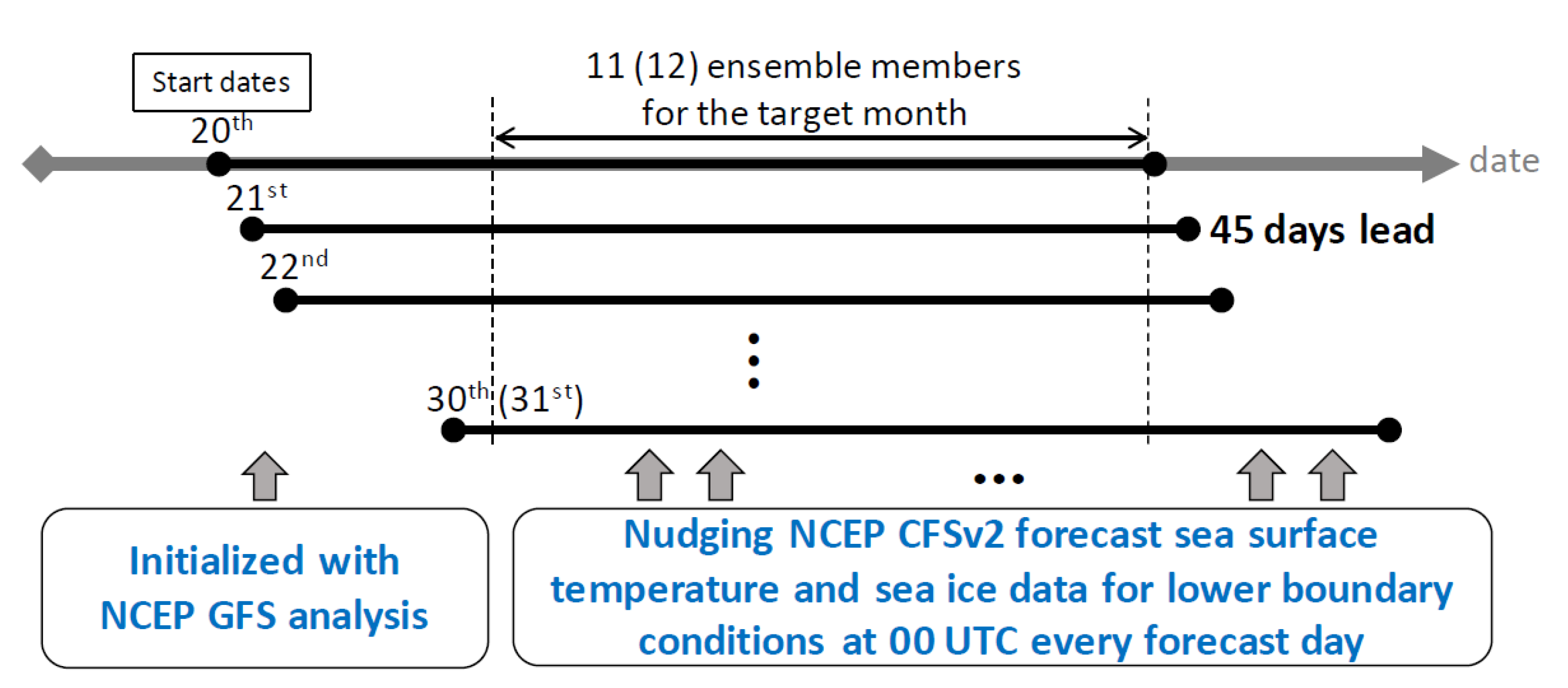
2.1. Model Settings and Experiment Design

A series of hindcast experiments are made for simulating EAWM from 2011 to 2020. A non-hydrostatic global atmospheric model, Model for Prediction Across Scales (MPAS) version 7 [36], is used in this study. MPAS uses C-grid staggering method for state variables, and the entire globe is covered with unstructured centroidal Voronoi mesh. The hybrid terrain-following method is used for the height coordinate [37]. MPAS has been widely used to study synoptic and mesoscale weather systems [38,39], as well as typhoons [40,41], tropical disturbances [42], MJO [43] and also climate change [44]. Many studies have shown that MPAS is capable of predicting synoptic or mesoscale events through day 7 and may capture the mean state for extended weather forecasts.
This study simulates and analyzes the synoptic weather systems in winter from the perspective of the S2S timescale. The 30 km uniform horizontal resolution mesh is used, and the model top is set at 30 km with 55 model levels. The model physics include the New Tiedtke convective cumulus scheme [45], the Weather Research and Forecasting Model single-moment 6-class microphysics (WSM6) scheme [46], Yonsei University (YSU) planetary boundary layer parameterization [47], Monin–Obukhov surface layer parameterization, the Noah land surface model, and the Rapid Radiative Transfer Model for GCM applications (RRTMG) longwave and shortwave radiation parameterizations [48].
Figure 1 is the schematic diagram of the hindcast experiments. Totally 315 45 day hindcasts are made for December, January, and February (DJF) from 2011 to 2020. Each hindcast is initialized with the analysis data of the National Centers for Environmental Prediction (NCEP) Global Forecast System (GFS) on 0.25° × 0.25° grids [49]. The 45 day hindcasts start at 00 UTC from 20 to 30 (31) in November, December and January. The NCEP Climate Forecast System Version 2 [50] forecast sea surface temperature (SST) and sea-ice data are used as lower boundary conditions at 00 UTC for every simulation day. There are 11 ensemble members for December and 12 ensemble members for January and February that construct time-lagged ensembles. The strategy of time-lagged ensembles has been studied and applied in different ranges of forecasts from 1–3 h up to 6–15 days. The time-lagged ensemble method can improve the forecast skill of deterministic forecast and provide probabilistic forecasts [51,52,53,54,55,56,57,58,59,60,61]. There are several methods of selecting different weights to generate the ensemble mean [53,62]. However, the equally weighted ensemble method is used as a first approach to analyze the performance of target months. In this study, monthly will be referred to the target month, and week 1–week 4 will be referred to the first to the fourth week in the target month.

2.2. Verification Data and Methods

The evaluating domain is defined from 5° S–55° N, 60° E–180° which covers Taiwan and most of East Asia. The 0.5-degree resolution CFSv2 analysis data (hereafter, CFSR) [50] are used to verify the MPAS hindcast results at specific pressure levels. The output frequency is four times a day (00, 06, 12, 18 UTC) for analysis and MPAS data. The model rainfall is verified with 0.1-degree resolution daily precipitation data retrieved from Global Precipitation Measurement (GPM) products [63,64]. The MPAS and GPM data were first remapped to the same grid as CFSR (0.5° × 0.5° grids) and averaged to obtain the monthly or weekly data according to the target evaluation time.
For long-range forecasts, it is common to use three-category climate outlook products in operational institutes [65]. The model grid data can be classified as “below normal”, “near normal” and “above normal” terciles. The three-category contingency table (Table 1) is usually used to verify the probability forecast performance. The Gerrity skill score (GSS) [66] is an equitable skill score which in a similar form to the Peirce skill score [67] and Heidke skill score [68]. The GSS can be defined as Equations (1)–(3). Here Pij is the sample probabilities of nine situations in the contingency table, N is the total sample size, Sij is the scoring matrix based on the equiprobable climatological categories. GSS is the probabilities multiplied by the scoring matrix, which ranged from −1 to 1. The perfect score is 1, and 0 represents no skill.
  G S S = i = 1 3 j = 1 3 P i j S i j ,
  P i j = n i j / N ,
  S i j = [ 1.25 0.25 1 0.25 0.5 0.25 1 0.25 1.25 ] ,
The probability forecasts of three-category monthly outlooks are evaluated using the relative operating characteristic curves (ROC) [69,70,71,72,73,74,75], and the reliability diagrams [75,76,77] with the Brier score (BS) [78,79,80] and the Brier skill score (BSS) [75,80]. ROC curve is a plot of hit rate (true positive rate) and false alarm rate (false positive rate) for all given cut-off thresholds. The area under the ROC curve (AUC) is also calculated to measure the predictive ability. The cut-off thresholds are defined from 0.1 to 0.9 every 0.1 in this study. It measures the ability of our probability forecasts for detecting the occurrence probability of below normal, near normal, and above normal events in our ensembles. In this study, the total sample size is 262,449, including all horizontal grids over 9 years.
The reliability diagrams show the observed frequency against the forecast probability. The BS is the mean square error of probability forecasts for binary events. The BSS is the forecast skill form of BS which references climatology:
B S = 1 N i = 1 N ( p i o i ) 2 ,
  B S S = B S B S c l i m 0 B S c l i m = 1 B S B S c l i m ,
  B S c l i m = o c l i m ( 1 o c l i m ) ,
here N is the sample size, pi is the forecast probability, oi is the observed frequency, and BSclim is the BS of climatological frequency. A BSS of 1.0 represents a perfect score, 0.0 for the reference state, and less and equal 0.0 indicates no skill. Curves close to the diagonal representing the predicted probabilities are more reliable corresponding to the observed frequencies.

3. Results

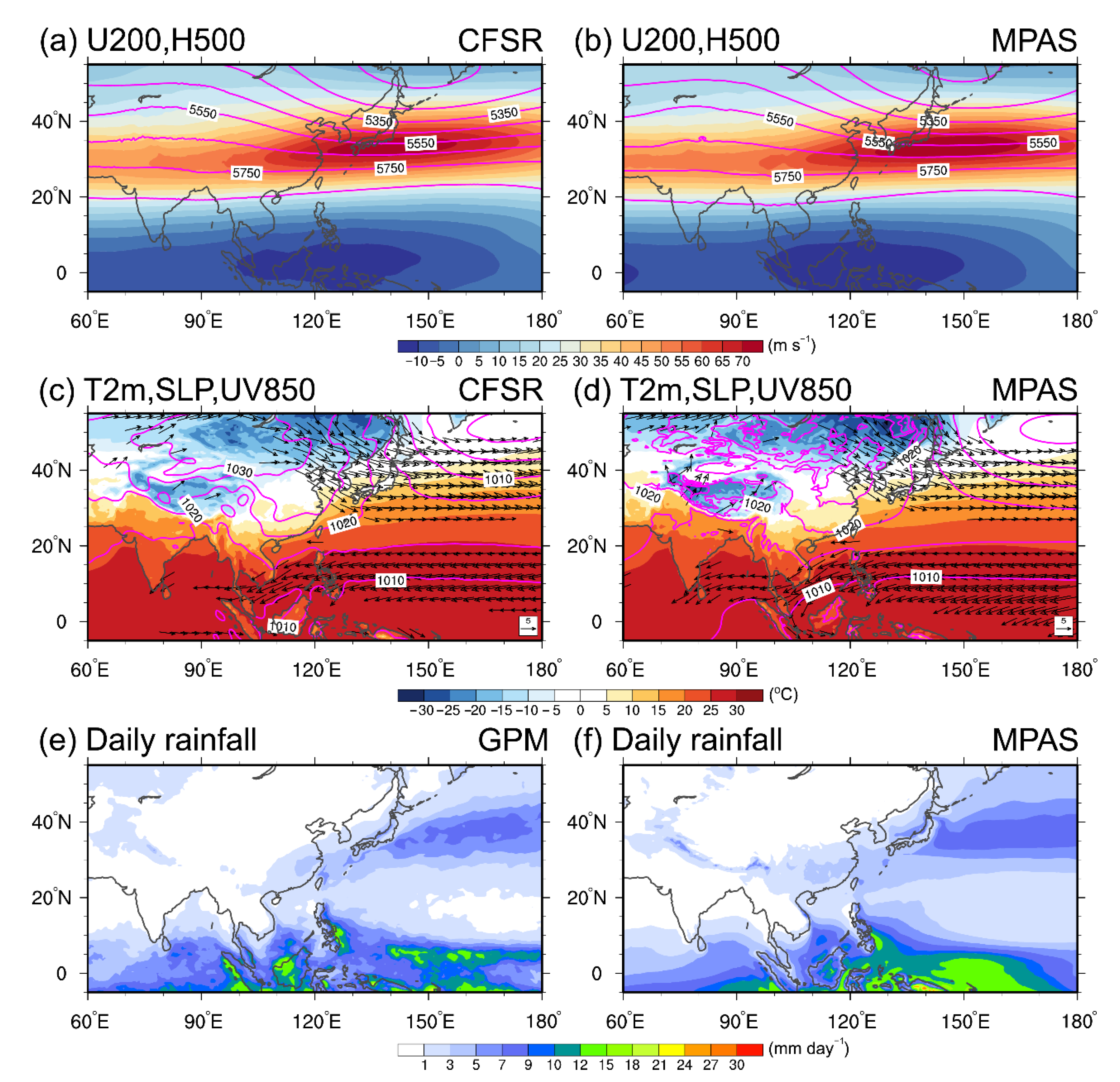
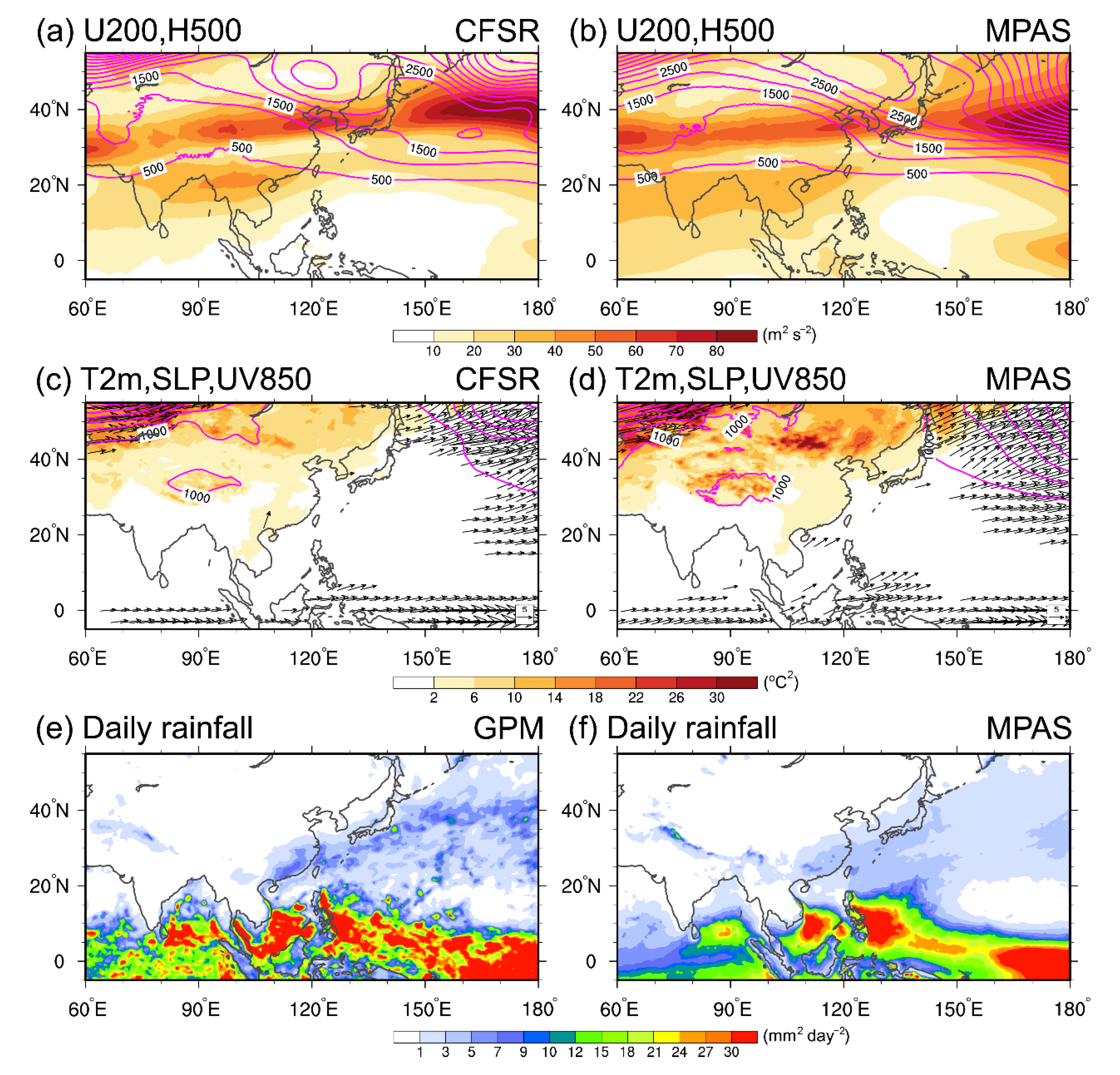
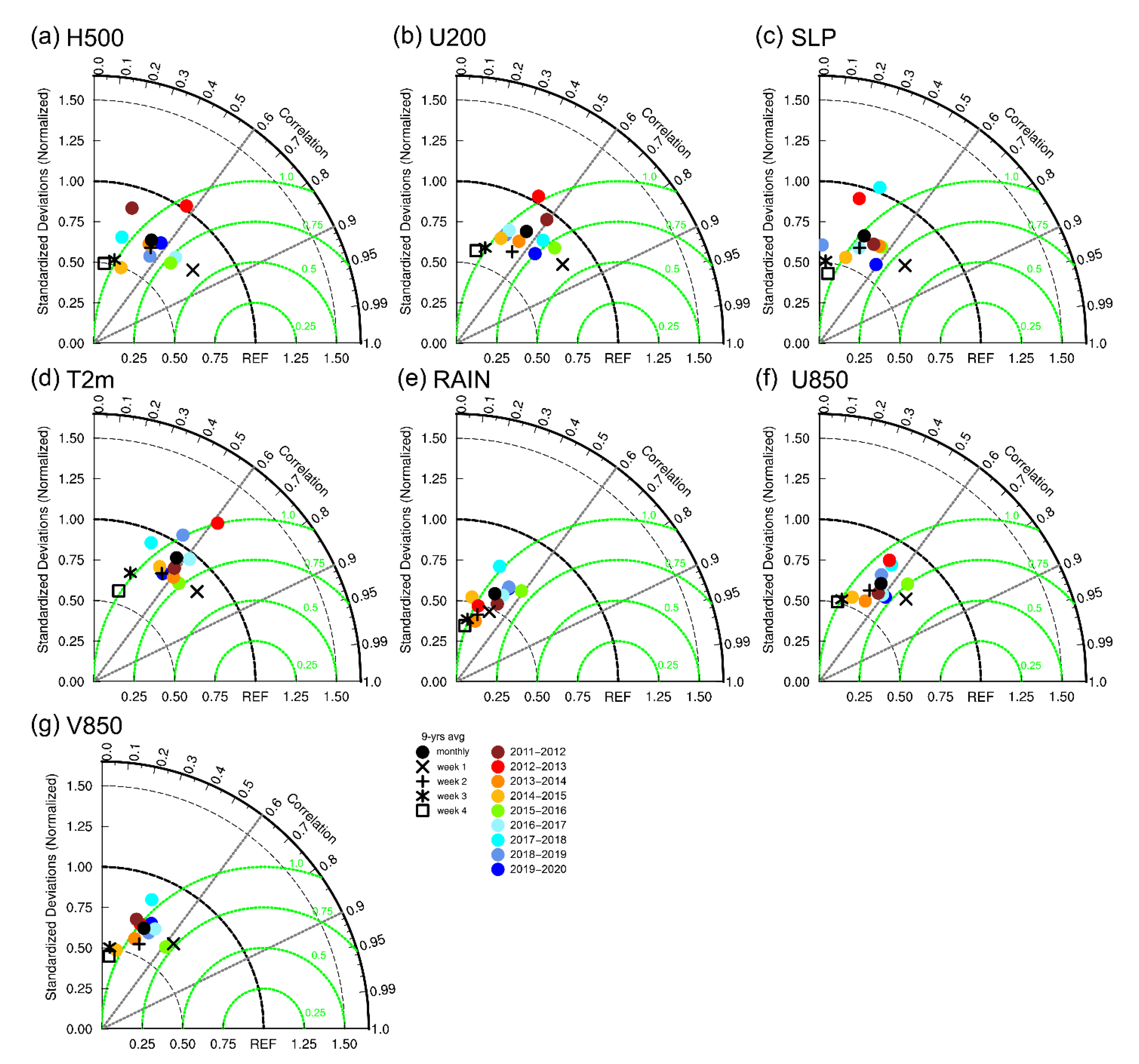
3.1. Climatology and Anomalies Verification

The climatology over 2011–2020 demonstrates consistent characteristics with typical EAWM patterns. The East Asian trough near the coast of East Asia and a strong East Asian westerly jet located in southern Japan are the most prominent features in the mid and upper troposphere (Figure 2a). The Siberian High and Aleutian Low dominate in the surface (Figure 2c). The mean daily rainfall is most significant in the South China Sea and the western Pacific in the tropics (Figure 2e). The second significant rainfall area locates at 30–40° N, 120° E–180 in mid-latitudes.
MPAS simulated climatology also captures these features (Figure 2b,d,f). The correlation coefficients (R), normalized root-mean-square errors (NRMSE), and mean bias are listed in Table 2. The NRMSE is the root-mean-square error normalized by the observed standard deviation [81]. Seven variables are selected to verify the model performance, 500-hPa geopotential height (H500), 200-hPa zonal wind (U200), sea-level pressure (SLP), 2-m temperature (T2m), 850-hPa zonal wind (U850), 850-hPa meridional wind (V850), and daily rainfall (RAIN). Table 2 indicates that the correlation coefficients are in general greater than 0.9 except for V850 and RAIN, which also exceed 0.871 and 0.898. Individually, the MPAS has more skill in simulating H500, U200, and T2m. The SLP, RAIN and 850-hPa winds have larger NRMSE. The mean bias of T2m is −0.58 °C, and the mean bias of simulated daily rainfall is about 0.32 mm day−1. Figure 2f also indicates that the climatological rainfall in MPAS is larger than the GPM-retrieved rainfall in most small rainfall areas. Additionally, MPAS simulates stronger northeasterly 850-hPa winds in most of our experiments (a negative bias in 850-hPa winds). Figure 3 evaluates the interannual variances. MPAS also captures the spatial distributions of variances (R exceeds 0.9 for H500, SLP, T2m, and U850, whereas R exceeds 0.8 for U200, V850, and RAIN), and most of the mean biases of simulated interannual variances are positive except for RAIN.
We further evaluate the ensemble mean performance for the H500, U200, SLP, T2m, RAIN, U850, and V850 anomalies by Taylor diagrams (Figure 4). Colors are the monthly mean of 2011–12 to 2019–20 DJF results. Black dots, crosses, plus, asterisks, and squares are 9-years averaged scores of monthly, week 1, week 2, week 3, and week 4, respectively. All the variables are standardized to obtain the R (azimuthal angle), the standardized deviation (radial distance) and the NRMSE (green circle). Most of the R for the monthly mean is between 0.4–0.6 but varies with years. The normalized standard deviation and NRMSE are about 0.5–0.75 and 0.75–1.0. The score decays from week 1 to week 4 due to the numerical predictability. The R of week 1 simulations can exceed 0.8 for H500 and U200 and exceed 0.7 for SLP, T2m, and U850. The scores of the monthly mean are approaching those of week 2. Among these variables, the R of the monthly mean can exceed 0.5 except for RAIN and V850. The Taylor diagram results indicate that the predictability decays quickly after 7 days in numerical weather forecasts. In the next section, we further examine the probability forecast results of our ensemble members on the S2S timescale.

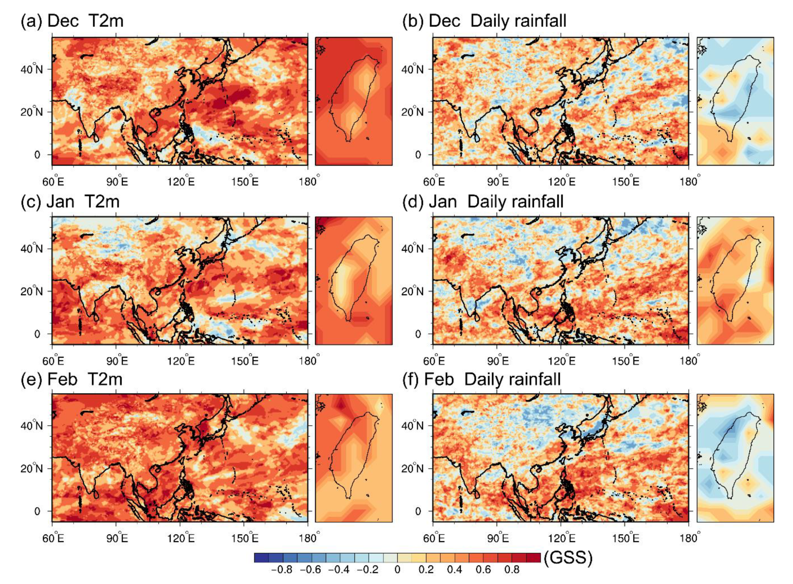
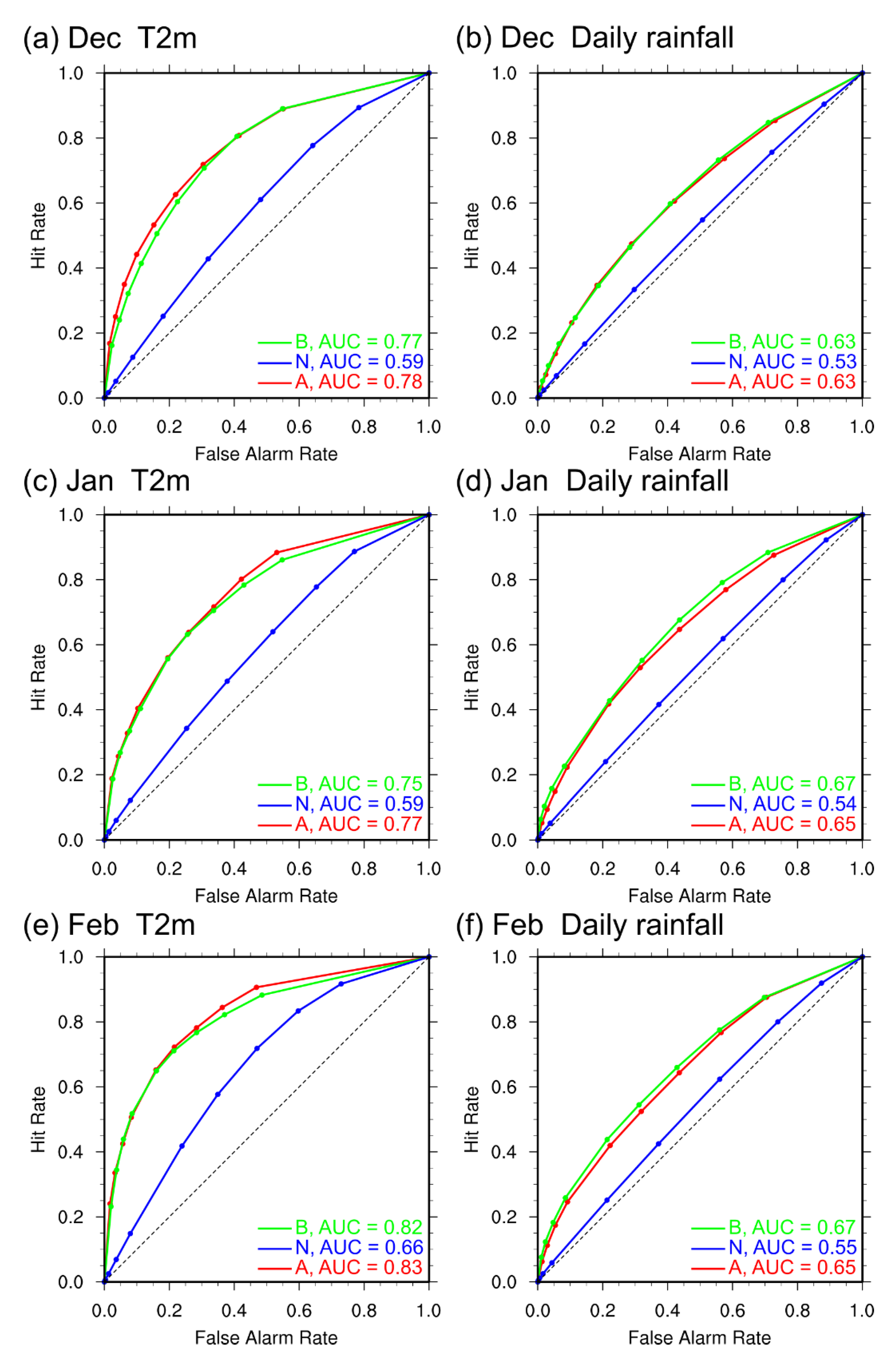
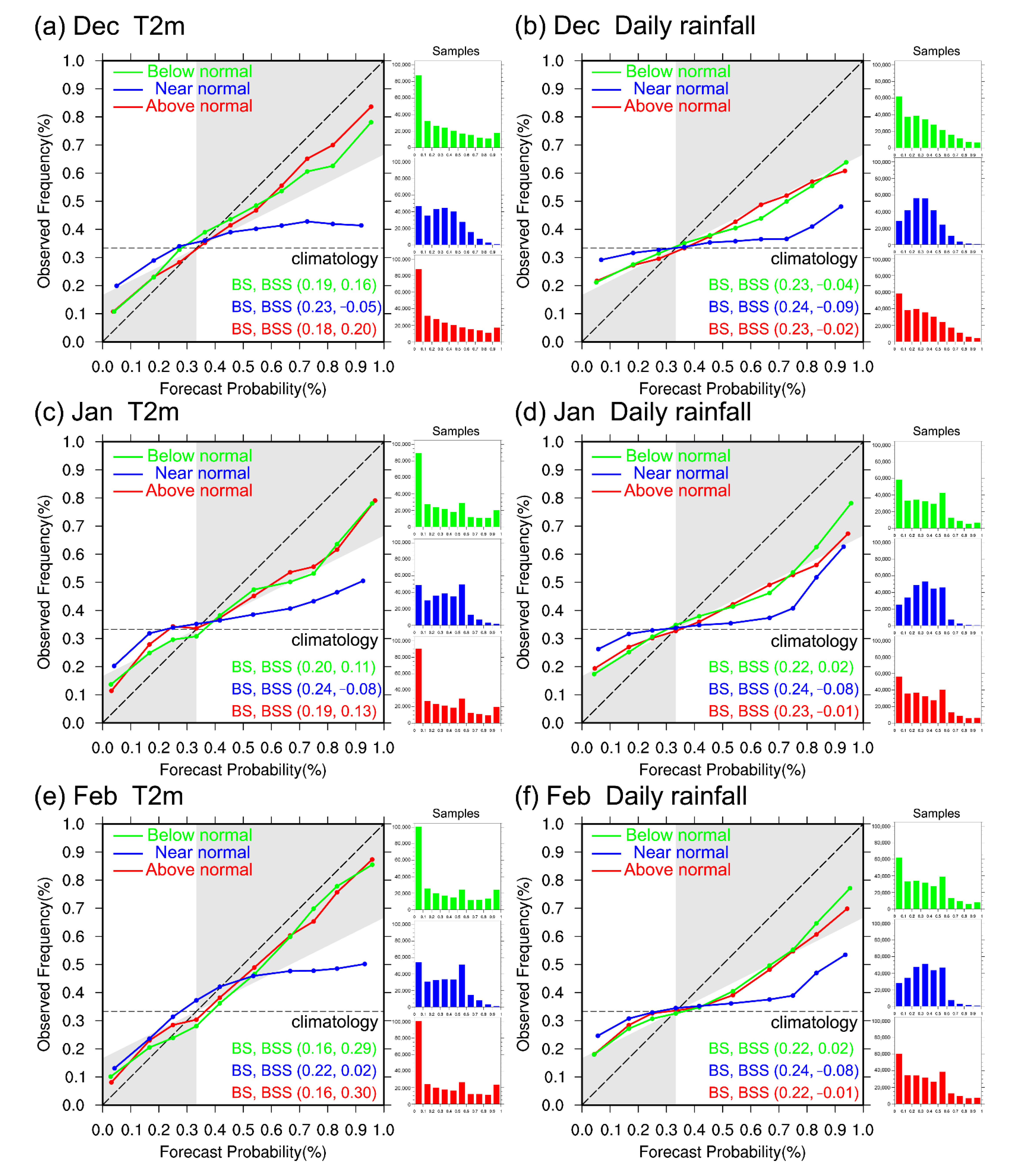
3.2. Three-Category T2m and Rainfall Probability Forecast Verification

Figure 5 shows the GSS of monthly averaged T2m and daily rainfall of MPAS ensemble mean for DJF over 2011–2020. In general, the MPAS ensemble mean has skill (positive GSS) in forecasting three-category T2m in most of East Asia during DJF. For rainfall, MPAS has higher GSS skills in the tropics than that in mid-latitude. For example, the GSS is positive in Western Pacific, South China Sea, and Indochina Peninsula, while most of the areas at about 40° N, 100–140° E have negative GSS. The GSS results also show large variability in Taiwan during DJF. Figure 5 indicates that MPAS has skill in forecasting rainfall in western, entire, and eastern Taiwan for December, January, and February, respectively. However, it also shows that MPAS has no skills in eastern and western Taiwan for December and February. The spatial composite GSS for individual ensemble members are similar to the ensemble mean results but generally have lower skill scores (figures not shown).
Figure 6 shows the ROC curves for monthly averaged T2m and rainfall. It indicates that T2m probability forecasts’ skill is in general better than that in rainfall. Among the three categories, the skills of below normal and above normal categories are better than those of the near normal category for both T2m and rainfall. The AUCs of below normal and above normal are approximately 0.75–0.83 for T2m and 0.63–0.67 for rainfall. The AUCs of near normal category are about 0.6 and 0.55 for T2m and rainfall.
Figure 7 shows the reliability diagrams with the BS and the BSS. Curves in the gray zone indicate that the forecasts have skills (better than climatology and contribute positively to BSS). Our results indicate that the forecast skills of below and above normal events are more reliable than near normal events. The near normal forecasts have lower resolution. The curves of T2m forecasts are in general sharper than that of rainfall, which implies that T2m forecasts are more reliable and have a better resolution to detect below normal and above normal events. In detail, the curves of T2m and rainfall all indicate that MPAS tends to over-forecasting for probabilities below 0.3 and under-forecasting for probabilities above 0.3.

3.3. Surface Temperature EOF Modes

Two leading EOF modes of surface air temperature over East Asian winter are important indicators for evaluating the model performance [4,7,32,82,83]. They are known as the northern and the southern modes. The northern mode (first EOF mode) is characterized by a westward shift of the East Asian trough and the moving of cold air from Siberia to northern East Asia. The major cooling is located at around 40–60° N. On the contrary, the major cooling occurs at the south of 40° N for the southern mode (second EOF mode). The cold air can extend to southern China and the South China Sea due to the deepening of the East Asian trough.
The normalized principal components of two leading EOF modes over the 2011–2020 winter for CFSR and MPAS ensemble mean are shown in Figure 8. The first and second EOF modes explain 37.8% (51.2%) and 14.8% (12.1%) of the temperature variance for CFSR (MPAS) over East Asia. The correlation coefficients for the first principal component (PC1) and the second principal component (PC2) are 0.60 and 0.35. The days that normalized principal components greater than 1.0 standard deviation are defined as significant PC1 and PC2 events. CFSR has 124 days and MPAS has 93 days of significant PC1 events over 2011–2020 DJF. For the month distribution of these PC1 event days, December, January, and February respectively occupy 19%, 58%, and 23% for CFSR while those for MPAS occupy 12%, 45%, and 43%. By contrast, MPAS has overestimation in February and underestimation in January. As for the significant PC2 events, there are 136 days for CFSR with 26%, 37%, and 37% in three separate months and 104 days for MPAS with 32%, 36%, and 32%. MPAS has a slight underestimation in both January and February. In summary, the MPAS ensemble mean underestimates the total number of significant PC1 and PC2 events. Individually, MPAS tends to overestimate PC1 events and underestimate PC2 events in February.
The difference between the composite anomalies of PC1 and PC2 greater than 1.0 and less than −1.0 standard deviation is shown in Figure 9 and Figure 10. MPAS simulates reasonable temperature patterns for the northern and the southern modes, with R = 0.93 and 0.83, respectively (Figure 9a,c and Figure 10a,c). However, the magnitude of the cooling temperature is underestimated. MPAS also captures the features of SLP, with R = 0.89 and R = 0.85 for the northern and the southern modes. The positive SLP anomalies are consistent with the surface temperature, which is located at the north (south) of 40° N for the first (second) mode. MPAS also captures the features in the upper troposphere. The R of U200 and H500 exceed 0.91 (0.93) and 0.97 (0.85) for PC1 (PC2). For PC1, negative H500 anomalies located near Korea and Japan, and positive U200 anomalies located at about 30° N imply that a significant westward-moving East Asian trough is accompanied by a strong East Asian westerly jet (Figure 9b,d). For PC2, the negative H500 anomalies extended southward to the south of 30° N, which indicates the deepening of the East Asian trough. The deepening of the East Asian trough also coincided with the southward moving positive SLP anomalies and results in the intensification of northeasterly winds and colder surface temperatures near Taiwan (Figure 10a,c).

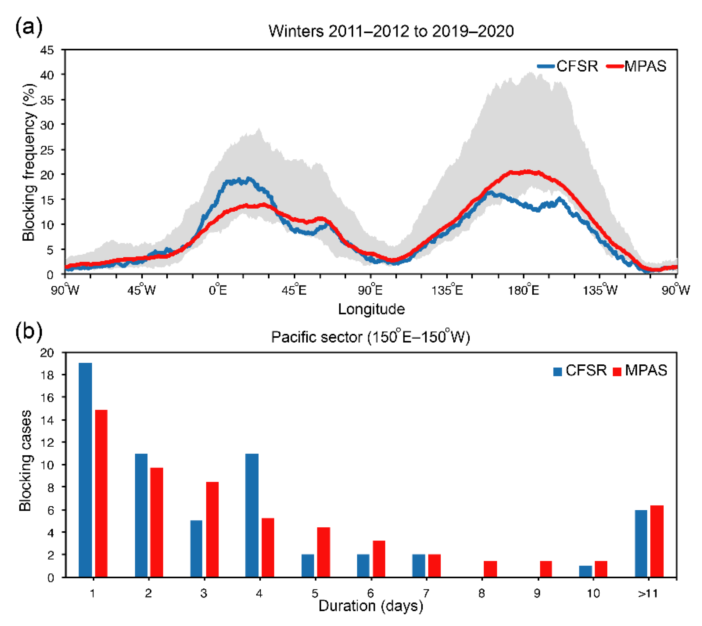
3.4. Atmospheric Blocking

Atmospheric blocking is an important feature to influence the EAWM. The blocking frequency as a function of longitude has two peaks over the Euro-Atlantic and Pacific region [84,85,86,87]. The blocking patterns are associated with the outbreaks of cold air from the Arctic area in winter. These cold air outbreaks would enhance the Siberian High and amplify the deepening of the East Asian trough, resulting in extreme cold events in East Asia [8,17,20,35,88]. The blocking is typically a closed high near 60° N with a positive geopotential height gradient at the south and increases the negative geopotential height gradient at the north. We follow the method reported in [85,86] to detect the blocking events in our experiments. First, the southern 500-hPa geopotential height gradient (GHGS) and the northern 500-hPa geopotential height gradient (GHGN) are calculated at each longitudinal grid point:
G H G S = Z 500 ( φ o ) Z 500 ( φ s ) φ o φ s ,   G H G N = Z 500 ( φ n ) Z 500 ( φ o ) φ n φ o ,
  φ n = 80 ° N + Δ ,   φ o = 60 ° N + Δ ,   φ s = 40 ° N + Δ ,   Δ = 5 ° , 0 ° , 5 ° ,
For any value of Δ that satisfies the conditions below, the given longitudinal grid is said to be blocked:
  G H G S > 0 ,   G H G N < 10 ,
The Pacific sector is also defined by the longitude band from 150–210° E. The sector is said to be blocked if the grid points are blocked extended for at least 10° longitudes.
The blocking frequency for our simulations over 2011–2020 DJF is shown in Figure 11a. MPAS simulations capture the typical features of two peaks of blocking frequency at about 0–30° E and 150–210° E. The average frequency is about 15–20%, which is consistent with the CFSR. MPAS time-lagged ensembles simulate the reasonable blocking frequency on the monthly time scale. The frequency can range from a minimum of 15% to a maximum of 40% for the Pacific sector and 10–25% for the Euro-Atlantic sector among our ensemble members. We further examine the averaged blocking cases as a function of durations for the Pacific sector (Figure 11b). MPAS simulates the same distribution of blocking cases compared to the CFSR. Specifically, there are about 1–2 cases over-forecasted for duration over 5 days, and four cases under-forecasted for a 1-day duration.

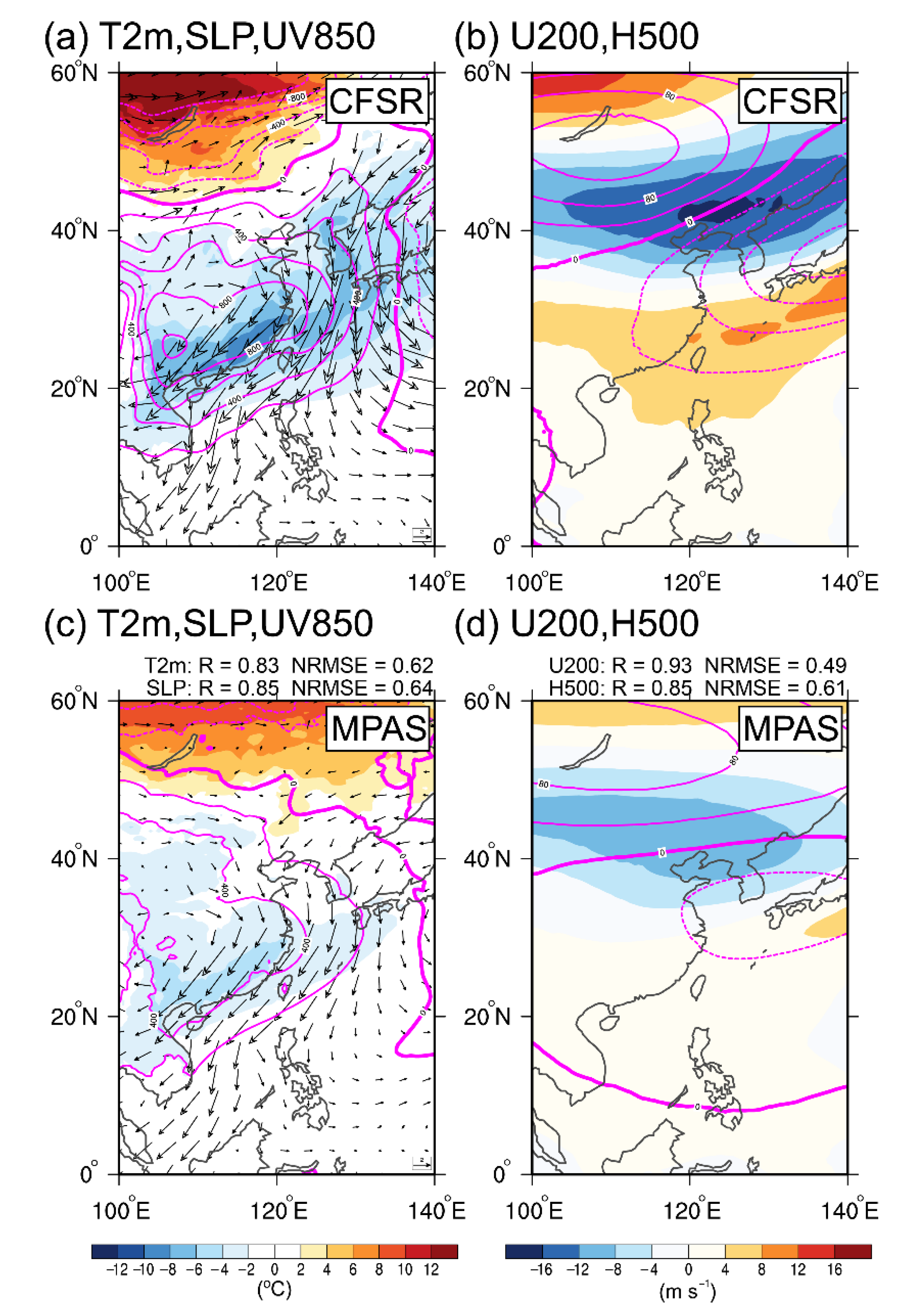
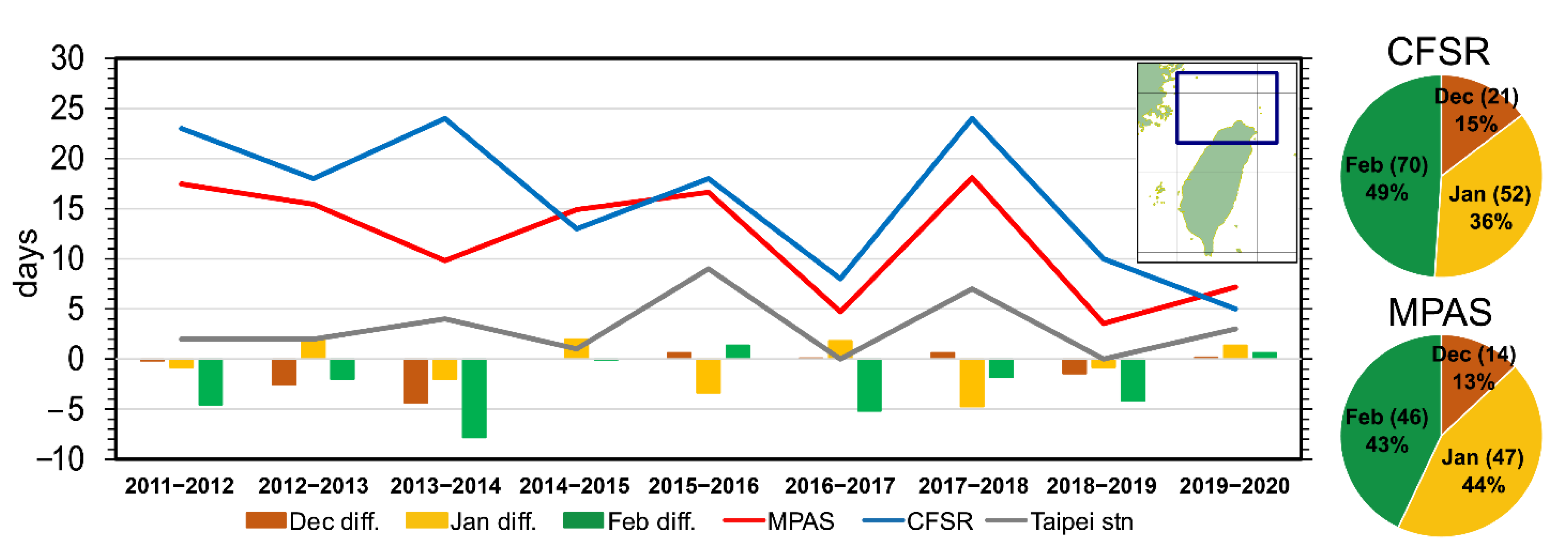
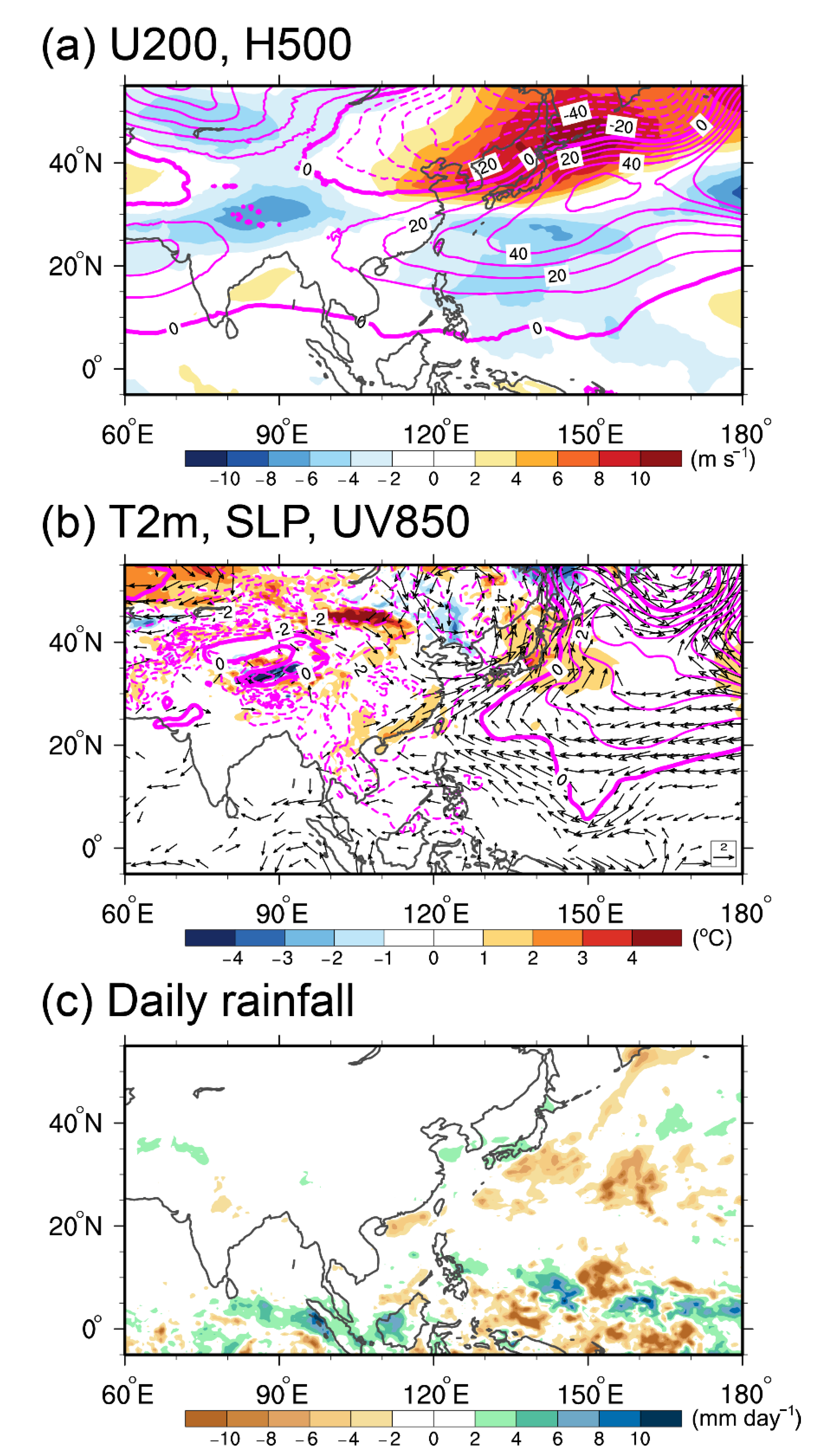
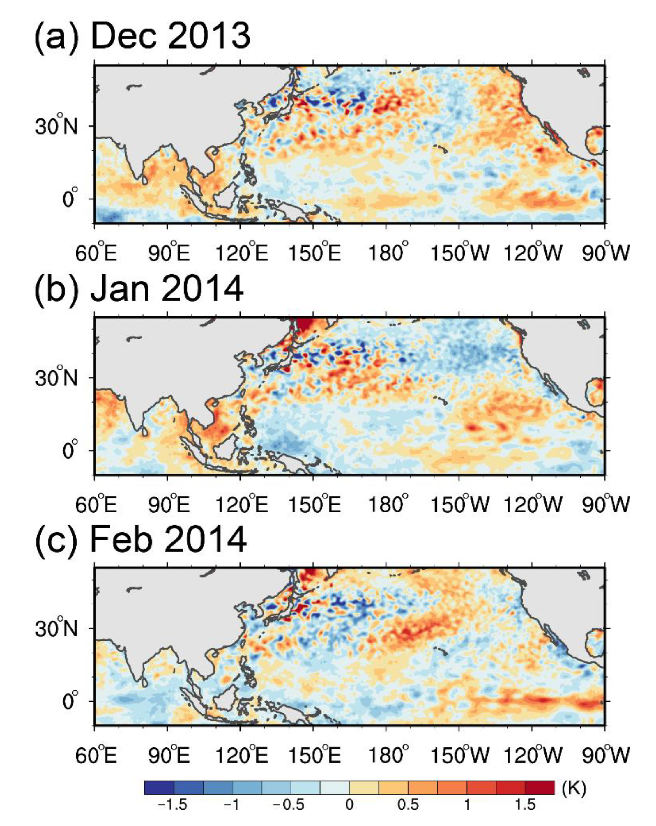
3.5. Investigation of Modeling Variability for the Cold Surge in Taiwan

Our EOF analyzed T2m patterns indicate that the cold air moves southward from EOF mode 1 to EOF mode 2 accompanied by northeasterly winds’ intensification. However, Taiwan is located in a transient region of about 23–25° N. Both these two modes may cause cold surge events in northern Taiwan. The Central Weather Bureau, Taiwan (CWB) defined the cold surge event in Taiwan by the criterion of daily temperature less than 10 °C at Taipei station. This operational criterion is difficult to apply to a global model due to our model resolution. Instead, we define the events as the minimum 2-m temperature less than 10 °C in the region of 24.75–26.5° N, 120–122.5° E, which is a looser criterion compare with the CWB definition. Figure 12 shows the annual occurrence frequency of cold surge events. The annual trend of CFSR (blue line) is consistent with that of Taipei station (gray line), but both CFSR and MPAS (red line) have more events. Figure 12 also shows that the annual trend of MPAS is similar to CFSR except for 2013–2014 DJF. The bars in Figure 12 are the event day differences between MPAS and CFSR in December (brown), January (yellow), and February (green). It indicates that the cold surge event days for MPAS are 24 days less than that of CFSR in February over 2011–2020. February 2014 has the most underestimation of 8 days among 9 years.
Figure 13a,b shows the composite differences for MPAS and CFSR in February 2014. Figure 13a indicates that the monthly mean East Asian trough tends to locate northern than 40° N with a stronger East Asian westerly jet located around Japan in MPAS. Accompanied with the upper tropospheric features are a weaker surface high anomaly in Eurasia and a stronger surface high anomaly in the Philippine Sea. The anomalous southwesterly winds to the west of this SLP anomaly thus reduce the strength of northeasterly winds near Taiwan (Figure 13b). Figure 14 shows the SST difference between the CFS forecast (also used as the lower boundary in MPAS) and CFSR during December 2013, January 2014, and February 2014. The monthly averaged SST used in MPAS is warmer than the reanalysis in the Eastern and Central Pacific during winter. This kind of SST distribution provides a similar effect with the establishment of the Philippine Sea anomalous anticyclone during El Niño [89]. This SST anomaly may also reduce the Walker circulation and produce the negative precipitation anomaly in the northwestern Pacific (Figure 13c). As a result, MPAS simulates a 2 °C warmer on average surface temperature and weaker northeasterly wind anomalies near Taiwan. The simulated trend of the westward-moving East Asian trough is also consistent with the results of Figure 8b. MPAS simulates the negative PC2 phase in February 2014, while CFSR is in a positive phase.

4. Conclusions

This study evaluates the model performance for simulating East Asian winter monsoon (EAWM) on subseasonal to seasonal (S2S) time scales. Model for Prediction Across Scales (MPAS) is used to conduct the hindcast experiments for DJF over 2011–2020 with 30 km horizontal resolution. An ensemble system is constructed with the time-lagged ensemble method, and the performance of the ensemble mean is analyzed. MPAS captures the features of EAWM climatology, such as the location of the East Asian trough and the East Asian westerly jet. The pattern correlations of seven selected variables (H500, U200, SLP, T2m, U850, V850, RAIN) are above 0.85. The mean bias of surface temperature and daily rainfall is −0.58 °C (−4.06%) and 0.32 mm day−1 (8.96%). The monthly and weekly mean anomalies are analyzed with Taylor diagrams. The correlation coefficients of week 1 simulations are about 0.8 for H500 and U200, and about 0.7 for SLP and T2m. The correlation coefficients drop quickly after week 1, but the monthly mean results are similar to week 2. The results are consistent with previous studies that the skill of the forecast for time averages can be greater than that of the instantaneous weather forecast at long range [90]. The correlation coefficients for the monthly mean are in general between 0.4–0.6, and the NRMSEs are about 0.75–1.0. The performance of daily rainfall is the worst among our selected variables. The correlation coefficients are in general below 0.5 even for the week 1 forecast.
The results of the three-category probability for monthly T2m and rainfall forecasts are further examined. The Gerrity Skill Scores (GSS) show that MPAS can make skillful T2m categories forecasts in most of East Asia during DJF 2011–2020. The GSS for monthly rainfall indicates that MPAS has higher skills in the tropics than that in mid-latitude, such as Western Pacific, South China Sea, and Indochina Peninsula. These regions also provide large interannual variability of rainfall during winter. MPAS has skills in Taiwan for January and has skills in western and eastern Taiwan for December and February. The ROC curve and reliability diagram analyze the accuracy and reliability of our three-category probability forecasts. In general, the probability forecasts of T2m are better than that of rainfall. Among the three categories, MPAS has more skill in detecting below normal and above normal events, and the forecasts are more reliable than those of the near normal category. However, MPAS still tends to over-forecasting (under-forecasting) for lower (higher) probability forecasts.
The EOF analysis is applied to the simulated surface temperature. MPAS reproduces the two leading modes and their associated circulations for EAWM, which represent the cold air located in northern East Asia or propagating into southern East Asia. The first and the second simulated EOF modes explain 63.3% of the temperature variance over East Asia, and the correlation coefficients for each principal component (PC1 and PC2) are 0.60 and 0.35, respectively. However, the MPAS ensemble mean tends to overestimate significant PC1 events and underestimate significant PC2 events in February. Atmospheric blocking index is chosen as another indicator to examine the model’s ability to simulate the synoptic features of EAWM. The forecast skills of blocking for climate models have been discussed in many studies. Most of the climate models can capture the distribution of Euro-Atlantic and Pacific sectors but may underestimate the blocking frequency [91,92,93]. MPAS reproduces the two peaks of blocking frequency at Euro-Atlantic and Pacific sectors and simulates the distribution of averaged blocking durations for the Pacific sector over the 2011–2020 winter.
Overall, MPAS captures the climatology, the major modes of EAWM variability, and the blocking activities. The evaluation results suggest that MPAS can produce skillful temperature probability forecasts and has the potential to predict extreme cases on S2S time scales. Many previous studies have shown the importance of AO and blocking to cold surge events in high latitudes, such as Japan, Korea, and northern China [17,20,21,22,23,24,35,88]. Since Taiwan is located in the subtropical region and the Western Pacific, ocean forcing may also play some roles to affect the occurrence chance of cold events through modulating the local circulation near Western Pacific. Our results show one of the possible mechanisms that influences the modeling variability of cold surge events in Taiwan. MPAS reproduces the annual trend of cold surge event days in Taiwan during 2011–2020 except in February 2014. We found that the Eastern and Central Pacific SSTs in MPAS are warmer than the reanalysis during DJF 2013–2014. This biased SST anomaly may reduce the strength of Walker circulation and enhance an anomalous anticyclonic high at the Philippine Sea. The associated southwesterly wind anomalies to the west of this anomalous high reduce the northeasterly winds near Taiwan. The weakening of the northeasterly winds might also reduce the occurrence numbers of the southern mode of surface temperature in our model. The association implies that the SST-forcing in the Western Pacific may affect the occurrence of cold events in Taiwan on S2S time scales. A fully coupled atmospheric-ocean model may play an important role in studying the interaction between the ocean and EAWM. It is also important to have longer hindcast data to verify the model’s capability for simulating El Niño/La Niña events.

Author Contributions

Conceptualization, L.-H.H., J.-L.C. and Y.-C.Y.; methodology, L.-H.H. and D.-R.C.; software, L.-H.H. and C.-C.C.; writing—original draft preparation, L.-H.H.; writing—review and editing, L.-H.H., C.-C.W. and J.-L.C.; project administration and funding acquisition, Y.-C.Y. All authors have read and agreed to the published version of the manuscript.

Funding

This research was supported by the Taiwan Ministry of Science and Technology through grants MOST-109-2119-M-865-004.

Institutional Review Board Statement

Not applicable.

Informed Consent Statement

Not applicable.

Data Availability Statement

The following institutes produce and host the repositories of the datasets analyzed in this study: NOAA (CFSv2 analysis, https://www.ncei.noaa.gov/data/climate-forecast-system/access/operational-analysis (accessed on 1 May 2020)), and NASA (GPM IMERG, https://gpm1.gesdisc.eosdis.nasa.gov/data/GPM_L3/GPM_3IMERGDF.06 (accessed on 1 May 2020)).

Acknowledgments

We thank National Center for High-performance Computing (NCHC) for providing computational and storage resources.

Conflicts of Interest

The authors declare no conflict of interest.

References

  1. Jhun, J.-G.; Lee, E.-J. A new East Asian winter monsoon index and associated characteristics of the winter monsoon. J. Clim. 2004, 17, 711–726. [Google Scholar] [CrossRef]
  2. Chan, J.C.L.; Li, C. The east Asian winter monsoon. In East Asian Monsoon; Chang, C.P., Ed.; World Scientific Publishing Company Incorporated: Singapore, 2004; pp. 54–106. [Google Scholar]
  3. Chang, C.-P.; Wang, Z.; Hendon, H. The Asian winter monsoon. In The Asian Monsoon; Wang, B., Ed.; Springer Praxis Books: Berlin/Heidelberg, Germany, 2006; pp. 89–127. [Google Scholar] [CrossRef]
  4. Wang, B.; Wu, Z.; Chang, C.P.; Liu, J.; Li, J.; Zhou, T. Another look at interannual-to-interdecadal variations of the East Asian winter monsoon: The northern and southern temperature modes. J. Clim. 2010, 23, 1495–1512. [Google Scholar] [CrossRef] [Green Version]
  5. Wang, L.; Lu, M.-M. The East Asian winter monsoon. In The Global Monsoon System: Research and Forecast, 3rd ed.; Chang, C.P., Kuo, H.C., Lau, N.C., Johnson, R.H., Wang, B., Wheeler, M., Eds.; World Scientific Publishing Company Incorporated: Singapore, 2017; pp. 51–61. [Google Scholar]
  6. Gong, H.; Wang, L.; Chen, W.; Wu, R.; Wei, K.; Cui, X. The climatology and interannual variability of the East Asian winter monsoon in CMIP5 models. J. Clim. 2014, 27, 1659–1678. [Google Scholar] [CrossRef]
  7. Li, J.; Wang, B.; Yang, Y.-M. Diagnostic metrics for evaluating model simulations of the East Asian Monsoon. J. Clim. 2020, 33, 1777–1801. [Google Scholar] [CrossRef]
  8. Joung, C.H.; Hitchman, M.H. On the role of successive downstream development in East Asian polar air outbreaks. Mon. Weather Rev. 1982, 110, 1224–1237. [Google Scholar] [CrossRef] [Green Version]
  9. Ding, Y. Build-up, air mass transformation and propagation of Siberian high and its relation to cold surge in East Asia. Meteorol. Atmos. Phys. 1990, 44, 281–292. [Google Scholar] [CrossRef]
  10. Gong, D.-Y.; Ho, C.-H. Intra-seasonal variability of wintertime temperature over East Asia. Int. J. Climatol. 2004, 24, 131–144. [Google Scholar] [CrossRef]
  11. Jeong, J.-H.; Kim, B.-M.; Ho, C.-H.; Chen, D.; Lim, G.-H. Stratospheric origin of cold surge occurrence in East Asia. Geophys. Res. Lett. 2006, 33, L14704. [Google Scholar] [CrossRef] [Green Version]
  12. Song, L.; Wang, L.; Chen, W.; Zhang, Y. Intraseasonal variation of the strength of the East Asian trough and its climate impacts in boreal winter. J. Clim. 2016, 29, 2557–2577. [Google Scholar] [CrossRef]
  13. Song, L.; Wu, R. Processes for occurrence of strong cold events over Eastern China. J. Clim. 2017, 30, 9247–9266. [Google Scholar] [CrossRef]
  14. Chen, W.; Yang, S.; Huang, R.H. Relationship between stationary planetary wave activity and the East Asian winter monsoon. J. Geophys. Res. 2005, 110. [Google Scholar] [CrossRef]
  15. Wang, L.; Huang, R.H.; Gu, L.; Chen, W.; Kang, L.H. Interdecadal variations of the East Asian winter monsoon and their association with quasi-stationary planetary wave activity. J. Clim. 2009, 22, 4860–4872. [Google Scholar] [CrossRef] [Green Version]
  16. Wang, L. Stationary wave activity associated with the East Asian winter monsoon pathway. Atmos. Ocean. Sci. Lett. 2014, 7, 7–10. [Google Scholar]
  17. Takaya, K.; Nakamura, H. Mechanisms of intraseasonal amplification of the cold Siberian high. J. Atmos. Sci. 2005, 62, 4423–4440. [Google Scholar] [CrossRef]
  18. Takaya, K.; Nakamura, H. Interannual variability of the East Asian winter monsoon and associated modulations of the planetary waves. J. Clim. 2013, 26, 9445–9461. [Google Scholar] [CrossRef]
  19. Liu, Y.; Wang, L.; Zhou, W.; Chen, W. Three Eurasian teleconnection patterns: Spatial structures, temporal variability, and associated winter climate anomalies. Clim. Dyn. 2014, 42, 2817–2839. [Google Scholar] [CrossRef]
  20. Takaya, K.; Nakamura, H. Geographical dependence of upper-level blocking formation associated with intraseasonal amplification of the Siberian high. J. Atmos. Sci. 2005, 62, 4441–4449. [Google Scholar] [CrossRef]
  21. Wu, B.; Wang, J. Winter Arctic oscillation, Siberian high and East Asian winter monsoon. Geophys. Res. Lett. 2002, 29, 1897. [Google Scholar] [CrossRef]
  22. Chen, W.; Kang, L. Linkage between the Arctic Oscillation and winter climate over East Asia on the interannual timescale: Roles of quasistationary planetary waves. Chin. J. Atmos. Sci. 2006, 30, 863–870. [Google Scholar]
  23. Chen, W.; Li, T. Modulation of Northern Hemisphere wintertime stationary planetary wave activity: East Asian climate relationships by the quasi-biennial oscillation. J. Geophys. Res. 2007, 112. [Google Scholar] [CrossRef]
  24. Jeong, J.-H.; Ho, C.-H. Changes in occurrence of cold surges over East Asia in associated with Arctic oscillation. Geophys. Res. Lett. 2005, 32, L14704. [Google Scholar] [CrossRef]
  25. Chang, C.-P.; Wang, Z.; Ju, J.; Li, T. On the relationship between western Maritime Continent monsoon rainfall and ENSO during northern winter. J. Clim. 2004, 17, 665–672. [Google Scholar] [CrossRef] [Green Version]
  26. Wang, B.; Wu, R.; Fu, X. Pacific–East Asian teleconnection: How does ENSO affect East Asian climate? J. Clim. 2000, 13, 1517–1536. [Google Scholar] [CrossRef]
  27. Jeong, J.-H.; Ho, C.-H.; Kim, B.-M.; Kwon, W.-T. Influence of the Madden-Julian Oscillation on wintertime surface air temperature and cold surges in East Asia. J. Geophys. Res. 2005, 110. [Google Scholar] [CrossRef]
  28. Jeong, J.-H.; Kim, B.-M.; Ho, C.-H.; Noh, Y.-H. Systematic variation in wintertime precipitation in East Asia by MJO-induced extratropical vertical motion. J. Clim. 2008, 21, 788–801. [Google Scholar] [CrossRef]
  29. White, C.J.; Carlsen, H.; Robertson, A.W.; Klein, R.J.; Lazo, J.K.; Kumar, A.; Vitart, F.; Coughlan de Perez, E.; Ray, A.J.; Murray, V.; et al. Potential applications of subseasonal-to-seasonal (S2S) predictions. Meteorol. Appl. 2017, 24, 315–325. [Google Scholar] [CrossRef]
  30. Alvarez, M.S.; Coelho, C.A.S.; Osman, M.; Firpo, M.Â.F.; Vera, C.S. Assessment of ECMWF subseasonal temperature predictions for an anomalously cold week followed by an anomalously warm week in central and southeastern South America during July 2017. Weather Forecast. 2020, 35, 1871–1889. [Google Scholar] [CrossRef]
  31. Taguchi, M. A study of false alarms of a major sudden stratospheric warming by real-time subseasonal-to-seasonal forecasts for the 2017/2018 northern winter. Atmosphere 2020, 11, 875. [Google Scholar] [CrossRef]
  32. Xiang, B.; Sun, Y.Q.; Chen, J.H.; Johnson, N.C.; Jiang, X. Subseasonal prediction of land cold extremes in boreal wintertime. J. Geophys. Res. Atmos. 2020, 125, e2020JD032670. [Google Scholar] [CrossRef]
  33. Vitart, F.; Ardilouze, C.; Bonet, A.; Brookshaw, A.; Chen, M.; Codorean, C.; Déqué, M.; Ferranti, L.; Fucile, E.; Fuentes, M.; et al. The Subseasonal to Seasonal (S2S) prediction project database. Bull. Am. Meteor. Soc. 2017, 98, 163–173. [Google Scholar] [CrossRef]
  34. Vitart, F.; Robertson, A.W. The sub-seasonal to seasonal prediction project (S2S) and the prediction of extreme events. Npj Clim. Atmos. Sci. 2018, 1, 3. [Google Scholar] [CrossRef] [Green Version]
  35. Gong, Z.; Feng, G.; Ren, F.; Li, J. A regional extreme low temperature event and its main atmospheric contributing factors. Theor. Appl. Clmatol. 2014, 117, 195–206. [Google Scholar] [CrossRef]
  36. Skamarock, W.C.; Klemp, J.B.; Duda, M.G.; Fowler, L.D.; Park, S.-H.; Ringler, T.D. A multiscale nonhydrostatic atmospheric model using centroidal Voronoi tessellations and C-grid staggering. Mon. Weather Rev. 2012, 140, 3090–3105. [Google Scholar] [CrossRef] [Green Version]
  37. Klemp, J.B. A terrain-following coordinate with smoothed coordinate surfaces. Mon. Weather Rev. 2011, 139, 2163–2169. [Google Scholar] [CrossRef]
  38. Schwartz, C.S. Medium-Range Convection-Allowing Ensemble Forecasts with a Variable-Resolution Global Model. Mon. Weather Rev. 2019, 147, 2997–3023. [Google Scholar] [CrossRef]
  39. Zhao, C.; Xu, M.; Wang, Y.; Zhang, M.; Guo, J.; Hu, Z.; Leung, L.R.; Duda, M.; Skamarock, W.C. Modeling extreme precipitation over East China with a global variable-resolution modeling framework (MPASv5.2): Impacts of resolution and physics. Geosci. Model Dev. 2019, 12, 2707–2726. [Google Scholar] [CrossRef] [Green Version]
  40. Davis, C.A.; Ahijevych, D.A.; Wang, W.; Skamarock, W.C. Evaluating medium-range tropical cyclone forecasts in uniform- and variable-resolution global models. Mon. Weather Rev. 2016, 144, 4141–4160. [Google Scholar] [CrossRef]
  41. Huang, C.-Y.; Zhang, Y.; Skamarock, W.C.; Hsu, L.-H. Influences of large-scale flow variations on the track evolution of Typhoons Morakot (2009) and Megi (2010): Simulations with a global variable-resolution model. Mon. Weather Rev. 2017, 145, 1691–1716. [Google Scholar] [CrossRef]
  42. Hsu, L.-H.; Tseng, L.-S.; Hou, S.-Y.; Chen, B.-F.; Sui, C.-H. A simulation study of Kelvin waves interacting with synoptic events during December 2016 in the South China Sea and Maritime Continent. J. Clim. 2020, 33, 6345–6359. [Google Scholar] [CrossRef]
  43. Pilon, R.; Zhang, C.; Dudhia, J. Roles of deep and shallow convection and microphysics in the MJO simulated by the Model for Prediction Across Scales. J. Geophys. Res. Atmos. 2016, 121, 10575–10600. [Google Scholar] [CrossRef] [Green Version]
  44. Michaelis, A.C.; Lackmann, G.M.; Robinson, W.A. Evaluation of a unique approach to high-resolution climate modeling using the Model for Prediction Across Scales—Atmosphere (MPAS-A) version 5.1. Geosci. Model Dev. 2019, 12, 3725–3743. [Google Scholar] [CrossRef] [Green Version]
  45. Zhang, C.; Wang, Y. Projected future changes of tropical cyclone activity over the Western North and South Pacific in a 20-km-mesh regional climate model. J. Clim. 2017, 30, 5923–5941. [Google Scholar] [CrossRef]
  46. Hong, S.-Y.; Lim, J.O.J. The WRF single-moment 6-class microphysics scheme (WSM6). J. Korean Meteor. Soc. 2006, 42, 129–151. [Google Scholar]
  47. Hong, S.-Y.; Noh, Y.; Dudhia, J. A new vertical diffusion package with an explicit treatment of entrainment processes. Mon. Weather Rev. 2006, 134, 2318–2341. [Google Scholar] [CrossRef] [Green Version]
  48. Iacono, M.J.; Delamere, J.S.; Mlawer, E.J.; Shephard, M.W.; Clough, S.A.; Collins, W.D. Radiative forcing by long-lived greenhouse gases: Calculations with the AER radiative transfer models. J. Geophys. Res. Atmos. 2008, 113, D13103. [Google Scholar] [CrossRef]
  49. National Centers for Environmental Prediction/National Weather Service/NOAA/U.S. Department of Commerce. NCEP Global Forecast System (GFS) Analyses and Forecasts. Research Data Archive at the National Center for Atmospheric Research, Computational and Information Systems Laboratory. 2007. Available online: https://rda.ucar.edu/datasets/ds084.6/ (accessed on 1 March 2020).
  50. Saha, S.; Moorthi, S.; Wu, X.; Wang, J.; Nadiga, S.; Tripp, P.; Behringer, D.; Hou, Y.T.; Chuang, H.Y.; Iredell, M.; et al. The NCEP Climate Forecast System Version 2. J. Clim. 2014, 27, 2185–2208. [Google Scholar] [CrossRef]
  51. Hoffman, R.N.; Kalnay, E. Lagged average forecasting an alternative to Monte Carlo forecasting. Tellus 1983, 35A, 100–151. [Google Scholar] [CrossRef]
  52. Branković, Č.; Palmer, T.N.; Molteni, F.; Tibaldi, S.; Cubasch, U. Extended-range predictions with ECMWF models: Time-lagged ensemble forecasting. Q. J. R. Meteorol. Soc. 1990, 116, 867–912. [Google Scholar] [CrossRef]
  53. Lu, C.; Yuan, H.; Schwartz, B.E.; Benjamin, S.G. Short-Range numerical weather prediction using time-lagged ensembles. Weather Forecast. 2007, 22, 580–595. [Google Scholar] [CrossRef]
  54. Mittermaier, M.P. Improving short-range high-resolution model precipitation forecast skill using time-lagged ensembles. Q. J. R. Meteorol. Soc. 2007, 133, 1487–1500. [Google Scholar] [CrossRef]
  55. Buizza, R. Comparison of a 51-member low-resolution (TL399L62) ensemble with a 6-member high-resolution (TL799L91) lagged-forecast ensemble. Mon. Weather Rev. 2008, 136, 3343–3362. [Google Scholar] [CrossRef] [Green Version]
  56. Ushiyama, T.; Sayama, T.; Tatebe, Y.; Fujioka, S. Numerical simulation of 2010 Pakistan flood in the Kabul River basin by using lagged ensemble rainfall forecasting. J. Hydrometeorol. 2014, 15, 193–211. [Google Scholar] [CrossRef]
  57. Jie, W.; Wu, T.; Wang, J.; Li, W.; Polivka, T. Using a deterministic time-lagged ensemble forecast with a probabilistic threshold for improving 6–15 day summer precipitation prediction in China. Atmos. Res. 2015, 156, 142–159. [Google Scholar] [CrossRef] [Green Version]
  58. Kim, K.-J.; Kim, Y.-O.; Kang, T.-H. Application of time-lagged ensemble approach with auto-regressive processors to reduce uncertainties in peak discharge and timing. J. Hydrol. Reg. Stud. 2017, 9, 140–148. [Google Scholar] [CrossRef]
  59. Xu, M.; Thompson, G.; Adriaansen, D.R.; Landolt, S.D. On the value of time-lag-ensemble averaging to improve numerical model predictions of aircraft icing conditions. Weather Forecast. 2019, 34, 507–519. [Google Scholar] [CrossRef]
  60. Khain, P.; Levi, Y.; Shtivelman, A.; Vadislavsky, E.; Brainin, E.; Stav, N. Improving the precipitation forecast over the Eastern Mediterranean using a smoothed time-lagged ensemble. Meteorol. Appl. 2020, 27, e1840. [Google Scholar] [CrossRef]
  61. Porson, A.N.; Carr, J.M.; Hagelin, S.; Darvell, R.; North, R.; Walters, D.; Mylne, K.R.; Mittermaier, M.P.; Willington, S.; Macpherson, B. Recent upgrades to the Met Office convective-scale ensemble: An hourly time-lagged 5-day ensemble. Q. J. R. Meteorol. Soc. 2020. [Google Scholar] [CrossRef]
  62. Van Den Dool, H.M.; Rukhovets, L. On the weights for an ensemble-averaged 6–10-day forecast. Weather Forecast. 1994, 9, 457–465. [Google Scholar] [CrossRef] [Green Version]
  63. Huffman, G.J.; Bolvin, D.T.; Braithwaite, D.; Hsu, K.; Joyce, R.; Kidd, C.; Nelkin, E.J.; Sorooshian, S.; Tan, J.; Xie, P. NASA Global Precipitation Measurement (GPM) Integrated Multi-Satellite Retrievals for GPM (IMERG), Algorithm Theoretical Basis Doc., Version 5.1. 2017; 34p. Available online: https://pmm.nasa.gov/sites/default/files/document_files/IMERG_ATBD_V5.1.pdf (accessed on 1 May 2020).
  64. Huffman, G.J.; Bolvin, D.T.; Nelkin, E.J. Integrated Multi-satellitE Retrievals for GPM (IMERG) Technical Documentation. NASA Doc. 2017; 54p. Available online: https://pmm.nasa.gov/sites/default/files/document_files/IMERG_doc.pdf (accessed on 1 May 2020).
  65. Jolliffe, I.T.; Stephenson, D.B. Forecast Verificaton: A Practitioner’s Guide in Atmospheric Science, 2nd ed.; Wiley-Blackwell: Oxford, UK, 2012. [Google Scholar]
  66. Gerrity, J.P., Jr. A note on Gandin and Murphy’s equitable skill score. Mon. Weather Rev. 1992, 120, 2707–2712. [Google Scholar] [CrossRef]
  67. Gandin, L.S.; Murphy, A. Equitable skill scores for categorical forecasts. Mon. Weather Rev. 1992, 120, 361–370. [Google Scholar] [CrossRef] [Green Version]
  68. Heidke, P. Berechnung des Erfolges und der Gute der Windstarkevorhersagen im Sturmwarnungsdienst (Measures of success and goodness of wind force forecasts by the gale-warning service). Geogr. Ann. 1926, 8, 301–349. [Google Scholar]
  69. Mason, S.J. A model for assessment of weather forecasts. Aust. Meteor. Mag. 1982, 30, 291–303. [Google Scholar]
  70. Harvey, L.O.; Hammond, K.R.; Lusk, C.M.; Mross, E.F. The application of signal detection theory to weather forecasting behavior. Mon. Weather Rev. 1992, 120, 863–883. [Google Scholar] [CrossRef] [Green Version]
  71. Mason, S.J.; Graham, N.E. Conditional probabilities, relative operating characteristics, and relative operating levels. Weather Forecast. 1999, 14, 713–725. [Google Scholar] [CrossRef]
  72. Mason, S.J.; Graham, N.E. Areas beneath the relative operating characteristics (ROC) and relative operating levels (ROL) curves: Statistical significance and interpretation. Q. J. R. Meteorol. Soc. 2002, 128, 2145–2166. [Google Scholar] [CrossRef]
  73. Kharin, V.V.; Zwiers, F.W. On the ROC score of probability forecasts. J. Clim. 2003, 16, 4145–4150. [Google Scholar] [CrossRef]
  74. Kharin, V.V.; Zwiers, F.W. Improved seasonal probability forecasts. J. Clim. 2003, 16, 1684–1701. [Google Scholar] [CrossRef]
  75. Wilks, D.S. Statistical Methods in the Atmospheric Sciences, 2nd ed.; Academic Press: Cambridge, MA, USA, 2006; p. 627. [Google Scholar]
  76. Hsu, W.-R.; Murphy, A.H. The attributes diagram: A geometrical framework for assessing the quality of probability forecasts. Int. J. Forecast. 1986, 2, 285–293. [Google Scholar] [CrossRef]
  77. Hamill, T.M. Reliability diagrams for multicategory probabilistic forecasts. Weather Forecast. 1997, 12, 736–741. [Google Scholar] [CrossRef]
  78. Brier, G.W. Verification of forecasts expressed in terms of probability. Mon. Weather Rev. 1950, 78, 1–3. [Google Scholar] [CrossRef]
  79. Murphy, A.H. A new vector partition of the probability score. J. Appl. Meteor. 1973, 12, 595–600. [Google Scholar] [CrossRef] [Green Version]
  80. Wilks, D.S. Sampling distributions of the Brier score and Brier skill score under serial dependence. Q. J. R. Meteorol. Soc. 2010, 136, 2109–2118. [Google Scholar] [CrossRef]
  81. Lee, J.-Y.; Wang, B. Future change of global monsoon in the CMIP5. Clim. Dyn. 2014, 42, 101–119. [Google Scholar] [CrossRef] [Green Version]
  82. Wu, Z.; Li, J.; Jiang, Z.; He, J.H. Predictable climate dynamics of abnormal East Asian winter monsoon: Once-in-a-century snowstorms in 2007/2008 winter. Clim. Dyns. 2011, 37, 1661–1669. [Google Scholar] [CrossRef]
  83. Lee, J.-Y.; Lee, S.-S.; Wang, B.; Ha, K.-J.; Jhun, J.-G. Seasonal prediction and predictability of the Asian winter temperature variability. Clim. Dyns. 2013, 41, 573–587. [Google Scholar] [CrossRef] [Green Version]
  84. Wallace, J.M.; Gutzler, D.S. Teleconnections in the geopotential height field during the Northern Hemisphere winter. Mon. Weather Rev. 1981, 109, 784–812. [Google Scholar] [CrossRef]
  85. Lejenäs, H.; Økland, H. Characteristics of northern hemisphere blocking as determined from a long time series of observational data. Tellus 1983, 35A, 350–362. [Google Scholar] [CrossRef]
  86. Tibaldi, S.; Molteni, F. On the operational predictability of blocking. Tellus 1990, 42A, 343–365. [Google Scholar] [CrossRef] [Green Version]
  87. Barriopedro, D.; García-Herrera, R.; Lupo, A.R.; Hernández, E.A. Climatology of Northern Hemisphere blocking. J. Clim. 2006, 19, 1042–1063. [Google Scholar] [CrossRef] [Green Version]
  88. Lu, M.-M.; Chang, C.-P. Unusual late-season cold surges during the 2005 Asian winter monsoon: Roles of Atlantic blocking and the Central Asian anticyclone. J. Clim. 2009, 22, 5205–5217. [Google Scholar] [CrossRef]
  89. Wang, B.; Zhang, Q. Pacific–East Asian teleconnection. Part II: How the Philippine Sea anomalous anticyclone is established during El Niño development. J. Clim. 2002, 15, 3252–3265. [Google Scholar] [CrossRef] [Green Version]
  90. Roads, J.O. Forecasts of time averages with a numerical weather prediction model. J. Atmos. 1986, 43, 871–892. [Google Scholar] [CrossRef] [Green Version]
  91. Scaife, A.A.; Woollings, T.; Knight, J.; Martin, G.; Hinton, T. Atmospheric blocking and mean biases in climate models. J. Clim. 2010, 23, 6143–6152. [Google Scholar] [CrossRef] [Green Version]
  92. Masato, G.; Hoskins, B.J.; Woollings, T. Winter and summer northern hemisphere blocking in CMIP5 models. J. Clim. 2013, 26, 7044–7059. [Google Scholar] [CrossRef]
  93. Jia, X.; Yang, S.; Song, W.; He, B. Prediction of wintertime Northern Hemisphere blocking by the NCEP Climate Forecast System. J. Meteorol. Res. 2014, 28, 76–90. [Google Scholar] [CrossRef]
Figure 1. Schematic diagram of the hindcast experiments. A series of 45 day hindcasts are made for December, January, and February from 2011 to 2020. Each hindcast is initialized with NCEP GFS analysis at 00 UTC from 20th to 30th (31st) in November, December and January. Totally 11 (12) ensemble members’ simulations that can cover the next month. During simulations, the NCEP CFSv2 forecast sea surface temperature and sea-ice data are used as model lower boundary conditions at 00 UTC every forecast day.
Atmosphere 12 00865 g001
Figure 2. Climatological DJF mean over 2011–2020 for (a,b) 200-hPa zonal wind (shaded) and 500-hPa geopotential height (contours), (c,d) 2-m temperature (shaded), sea-level pressure (contours), and 850-hPa winds (vectors), (e,f) daily rainfall (shaded). CFS reanalysis and GPM-retrieved rainfall (simulations) are listed at left (right) column.
Atmosphere 12 00865 g002
Figure 3. Same as Figure 2 but for the interannual DJF variances over 2011–2020 for (a,b) 200-hPa zonal wind (shaded) and 500-hPa geopotential height (contours), (c,d) 2-m temperature (shaded), sea-level pressure (contours), and 850-hPa winds (vectors), (e,f) daily rainfall (shaded). CFS reanalysis and GPM-retrieved rainfall (simulations) are listed at left (right) column.
Atmosphere 12 00865 g003
Figure 4. Taylor diagrams for (a) H500, (b) U200, (c) SLP, (d) T2m, (e) RAIN, (f) U850, and (g) V850 anomalies. Colors are the monthly mean of 2011–2012 to 2019–2020 DJF. Black dots, crosses, plus, asterisks, and squares are 9-years averaged scores of monthly, week 1, week 2, week 3, and week 4, respectively. Green circles are the normalized root-mean-square errors.
Atmosphere 12 00865 g004
Figure 5. Gerrity skill score (GSS) of monthly averaged T2m (left column) and averaged daily rainfall (right column) on (a,b) December, (c,d) January, and (e,f) February. The zoom-in area of Taiwan is listed on the right panel of each figure.
Atmosphere 12 00865 g005
Figure 6. The relative operating characteristic curves (ROC) and the area under the ROC curve (AUC) for the three-category probabilities of monthly averaged T2m (left column) and averaged daily rainfall (right column) on (a,b) December, (c,d) January, and (e,f) February. Green, blue, red lines denote the below normal (B), near normal (N), and above normal (A) categories.
Atmosphere 12 00865 g006
Figure 7. Reliability diagrams for the three-category probabilities of monthly averaged T2m (left column) and averaged daily rainfall (right column) on (a,b) December, (c,d) January, and (e,f) February. Green, blue, red lines denote the below normal, near normal, and above normal categories. The thin dashed line is 0.333 according to the observed frequency of climatology for the three-category method. The Brier score (BS) and the Brier skill score (BSS) are denoted at the right bottom of each figure.
Atmosphere 12 00865 g007
Figure 8. The normalized principal components of (a) the first EOF mode (PC1) and, (b) the second EOF mode (PC2) for CFS reanalysis (blue) and MPAS (red). The right column shows the observed and simulated days in December, January, and February for that PC1 and PC2 greater than 1.0 standard deviation.
Atmosphere 12 00865 g008
Figure 9. The difference between the composite anomalies of which PC1 greater than 1.0 and less than −1.0 standard deviation. (a,c) T2m, SLP, and 850-hPa winds. (b,d) U200 and H500. The upper row for the CFSR and the lower row for the MPAS ensemble mean.
Atmosphere 12 00865 g009
Figure 10. Same as Figure 9, but for PC2. (a,c) T2m, SLP, and 850-hPa winds. (b,d) U200 and H500. The upper row for the CFSR and the lower row for the MPAS ensemble mean.
Atmosphere 12 00865 g010
Figure 11. (a) Percentage frequency of blocking as a function of longitude for CFSR (blue) and MPAS simulations average (red). The shading area is defined by the minimum and maximum values of the ensemble members. (b) Histograms of the averaged blocking cases as a function of durations for the Pacific sector (150–210° E).
Atmosphere 12 00865 g011
Figure 12. Annual trend of cold events days for MPAS (red line), CFSR (blue), and Taipei station (gray). The cold events are defined as the minimum 2-m temperature less than 10 °C in the region of 24.75–26.5° N, 120–122.5° E for MPAS and CFSR. Bars represent the number of days between MPAS and CFSR in December (brown), January (yellow), and February (green). The pie chart shows the event days in December (brown), January (yellow), and February (green) for MPAS and CFSR.
Atmosphere 12 00865 g012
Figure 13. The differences between MPAS and CFSR in February 2014 for (a) U200 and H500, and (b) T2m, SLP, and 850-hPa winds. (c) Averaged daily rainfall difference between MPAS and GPM-retrieved rainfall in February 2014.
Atmosphere 12 00865 g013
Figure 14. Composite of the SST difference between CFS forecast (also used as the lower boundary in MPAS) and CFSR in (a) December 2013, (b) January 2014, and (c) February 2014.
Atmosphere 12 00865 g014
Table 1. Three-category contingency table. Pij is the sample probability, in which i, j are ranged from 1 to 3 and denotes the categories of forecast and observed, respectively.
CategoriesObserved
Below NormalNear NormalAbove Normal
ForecastBelow normalP11P12P13
Near normalP21P22P23
Above normalP31P32P33
Table 2. List of verification results for climatology. H500, U200, SLP, T2m, U850, V850, and RAIN are 500-hPa geopotential height, 200-hPa zonal wind, sea-level pressure, 2-m temperature, 850-hPa zonal wind, 850-hPa meridional wins, and daily rainfall, respectively.
VariablesCorrelation Coefficient (R)Normalized Root-Mean-Square Error (NRMSE)Mean Bias
H5000.9980.07−6.43 (m)
U2000.9980.070.04 (ms−1)
SLP0.9620.32−0.94 (hPa)
T2m0.9950.11−0.58 (°C)
U8500.9700.29−0.83 (m s−1)
V8500.8710.56−0.31 (m s−1)
RAIN0.8980.480.32 (mm day−1)
Publisher’s Note: MDPI stays neutral with regard to jurisdictional claims in published maps and institutional affiliations.

