Article

Flooding Risk Assessment and Analysis Based on GIS and the TFN-AHP Method: A Case Study of Chongqing, China

School of Management Science and Real Estate, Chongqing University, Chongqing 400044, China
*
Author to whom correspondence should be addressed.
Atmosphere 2021, 12(5), 623; https://doi.org/10.3390/atmos12050623
Submission received: 17 April 2021 / Revised: 8 May 2021 / Accepted: 10 May 2021 / Published: 12 May 2021
(This article belongs to the Section Climatology)

Abstract

:
Flood risk assessment and mapping is required for management and mitigation of flood in mountain cities. However, the specific characteristics of population, society, economy, environment, transportation and other disaster-bearing bodies in various regions of mountain cities are significantly different, which increases the uncertainty of risk assessment index weight and risk assessment accuracy. To overcome these problems, the triangular fuzzy number-based analytical hierarchy process (TFN-AHP) was employed to determine the weights of eleven indexes influencing flooding. Further, the geographic information system (GIS) spatial statistics technique was introduced to investigate global regional risk pattern, as well as to identify local risk hot spots. Experiments were conducted using open data of Chongqing, China. From the results, it was observed that the TFN-AHP has a higher efficiency in flood risk assessment on mountain cities than the AHP method. The dynamically changing risk pattern and risk hot spots were explored, and the results are generally consistent with seasonal characteristics of precipitation. Lastly, sensitivity analysis of assessment factors’ weights was conducted. The comparative consequences indicate that TFN-AHP can better assess the flooding risk and can be successfully applied to urban development policy.

1. Introduction

Floods are one of the most devastating natural disasters with considerable damage and significant socio-economic impact on different sectors that occur across the world [1]. The increase in the frequency of flooding can be associated with the impacts of climate change and rapid urbanization. Statistics revealed that flood accounts for 34% and 40% of all global natural disasters in quantity and in losses, respectively [2,3]. In China, more than 2000 floods have ravaged since the dawn of the 20th century, resulting in massive loss of life and finance that equates to an average year of 1254 deaths and 2 billion USD lost [4]. Therefore, there is an urgent need to conduct flooding risk assessment for risk reduction and disaster management purposes.
In recent years, a growing body of studies on flood risk assessment and analysis have been carried out in different regions and cities, such as plain cities and coastal cities [5]. For example, researchers used remote sensing (RS), GIS and open data (such as social media data, volunteer geographic information) to study the flood risk in Wuhan, coastal Mainland China and Europe [6,7,8]. However, comparatively little investigation has been performed on mountain cities. It is widely recognized that mountain cities are sensitive to sudden and defensive floods on account of large elevation disparity and other specific factors [9]. Just as Thaler et al. stated that different countries respond to flood disaster from different angels, Sakamoto et al. aimed to test the ability of forests in flood from a time-series perspective in the Cambodia and the Vietnamese Mekong Delta [10]. Williams et al. considered physical infrastructures and social conditions to measure the adaptive capacity of Alaskan communities in flood events [11]. Fan et al. employed population, flood arrival time, flood level, evacuation time and local GDP (Gross Domestic Product) to explore the flood quantitatively [12]. This problem stands out in China, with 33% mountainous land areas. For instance, on 20 June 2020, floods in Chongqing affected more than 150,000 people, causing direct economic losses of 29,977,000 USD Flood is the most dynamic natural disaster that cannot be absolutely prevented, but with flood risk assessment, its occurrence can be forecasted, and the damage can be alleviated.
To date, the use of GIS and RS, along with multi-criteria decision-making techniques, such as the analytic hierarchy process (AHP), have been explored in flood risk assessment of mountain cities [13,14]. Although previous approaches have gained great achievements in the field, they do not pay much attention to uncertainty of floods caused by specific environmental characteristics of mountain cities [15]. Take Chongqing as a case, there is significant variation on environment (such as elevation difference, surface coverage), socio-economic (such as population, built environment) and disaster-bearing bodies (such as transportation, facilities) in various regions [16]. These features greatly decrease the robustness of the risk assessment method, and further reduce the certainty of the weight of the assessment index and the accuracy of the assessment result. In flood risk assessment, the uncertainty of the AHP cannot be eliminated, but it can be mitigated with a proper flood predictive system. Thus, establishing a flood risk assessment method for mountain cities with minor uncertainty of the evaluation index weight as far as possible is an effective way to address the mentioned problems.
To diminish the damage caused by floods, several approaches have been applied in flood risk assessment. Generally speaking, the related research can be mainly divided into the following four categories [2]: The first is the historical data statistics method [17]. This method is applied to estimate flood risk through analyzing historical flood events’ data. However, it is difficult to have enough data to support long time-series and dynamic change analysis [18]. Second is the index system method [19]. This approach, such as the multi-criteria decision-making technique, considers the flood risk assessment as the result of comprehensive action of several assessment factors. However, the determination of risk assessment indicators primarily depends on judgements of experts with distinct favors [20]. Thereby, more accuracy problems are caused when exploring the spatial distribution of flood risk. The third category is the coupling of GIS and the RS method. This approach has been widely used in flood assessment and mapping [21]. The last category is the scenario simulation method [22]. This approach needs detailed topography and geomorphology data, and it is commonly applied in the prediction of flood risk in small regions [23]. Accordingly, the application of this method is limited owing to the fact that the floods usually occur at a large regional scale.
In the mentioned methods, the index-based methods with intelligence techniques are more appropriate to consider the uncertainties of natural disasters, where AHP is one of the approaches widely employed [24]. AHP can subdivide flood risk into special factors suitable for zones with various characteristics, which imposes obvious effects on practicability enhancement. Despite that AHP has been criticized for the high subjectivity inherent in experts’ judgments, it has been optimized by combining with several mathematical approaches, such as fuzzy logic methodology. Its integration with AHP has been used in flood risk evaluation, such as trapezoidal fuzzy AHP and TFN-AHP, among which TFN-AHP is the most efficient in that quite a few experts with a high variation of preferences are involved in complicated situations [25].
During the application of traditional AHP for flood risk assessment of mountain cities, which stand at an average elevation of 400 m with respect to sea level, the uncertainty that exists in human judgments and the pairwise comparisons of assessment factors are unavoidable [24]. Meanwhile, the specific environmental characteristics of mountain cities also contribute to uncertainty. Additionally, hazard, exposure and disaster resistance indicators have been less considered in previous studies [9]. Accordingly, TFN-AHP can not only inherit strengths of AHP to integrate assorted assessment indexes, but can minimize uncertainty through fuzzy numbers, which could prevent flood risk in mountain cities or at least minimize harmful influences.
Although we can get a sense of the overall regional flood risk distribution by mapping them, it is difficult for us to draw conclusions or find explicit answers directly from the flood risk maps, causing failures of present flood prevention action [26]. Hence, understanding the evolving characteristics of flood risk spatio-temporal pattern and risk clusters is key for risk effects reduction strategies for decision-making. In this context, some emerging questions, such as “where are the flood risk hot zones?” and “how is the flood risk spatio-temporal pattern?” should be first answered from a spatio-temporal perspective [27]. Thereby, not only analyzing the global risk distribution pattern, but also identifying risk hot spots from local scale and multiple time scales are indispensable for comprehensive flooding management [28].
Recently, in addition to flood risk mapping, risk classification [14], sensitivity analysis [1] and spatio-temporal model analysis [29] have been investigated in related research. For instance, with respect to time-series analysis, some works used the time-series method and GIS technology to explore the risk temporal pattern under the scales of year [30], season, month [31], week, daily and hourly. For the spatial patterns’ research scales, quite a few techniques have been employed in multidimensional investigation on different spatial scales [32,33]. Overall, the GIS spatial statistics technique (such as Moran’s I, LISA) is the most commonly adopted one to identify heterogeneity and agglomeration at diverse spatial scales.
Considering that TFN-AHP can enhance accuracy and GIS is useful in investigating spatial pattern, their utility has already been applied in disaster evaluation such as floods. In this paper, we incorporate the triangular fuzzy function into the original AHP method to weaken the uncertainty in the determination of risk index weights. Moreover, we apply the GIS spatial statistics technique in the spatio-temporal pattern. Three areas are explored: (i) the TFN-AHP method is introduced to cope with the uncertainty of flood risk assessment, (ii) the flood risk spatio-temporal distribution pattern is analyzed through the GIS spatial statistics technique and (iii) Chongqing is taken as an example to validate the efficiency of the TFN-AHP method and accurately identify flood-prone areas.

2. Materials and Methods

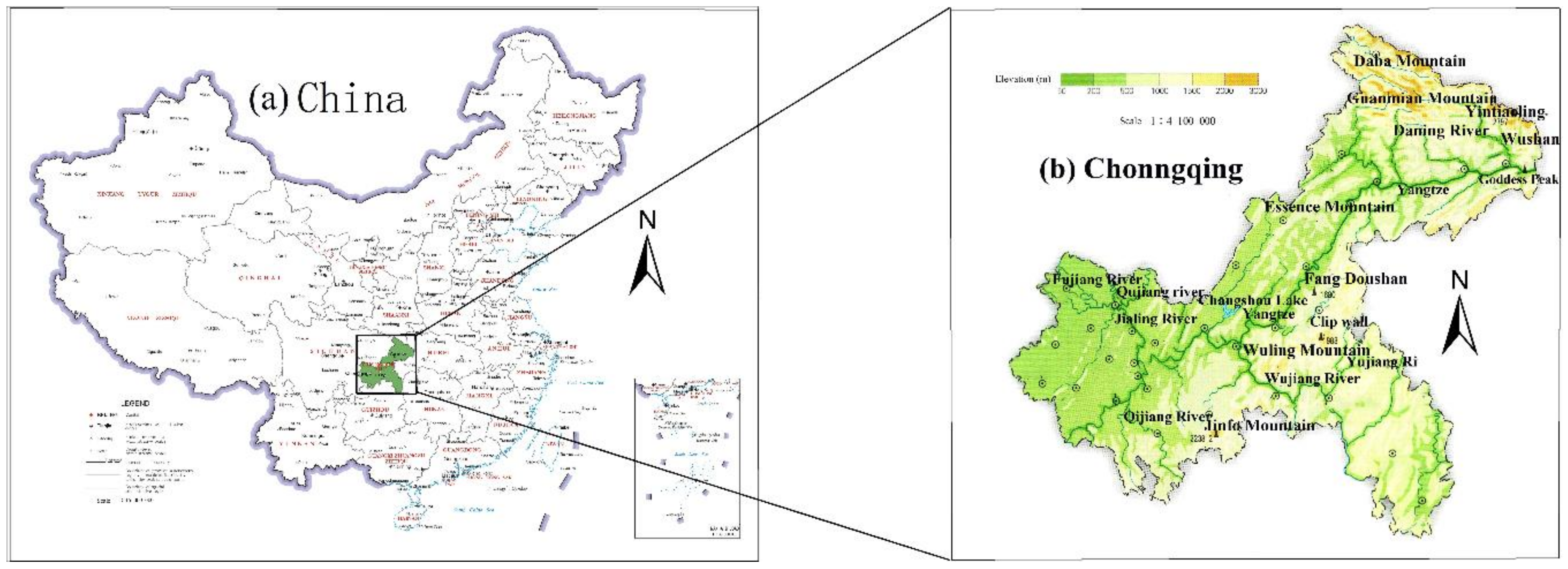
2.1. Study Area and Data

Chongqing is known as a mountain city, where mountains and hills account for 94% of land areas. Situated in the Middle-Lower Yangtze Plain, it belongs to the subtropical monsoon humid climate zone with profuse rainfall, and the annual precipitation in most areas ranges from 1000 to 1350 mm (Figure 1). The Yangtze River, Jialing River and Wujiang river flow through Chongqing, with an average annual total water resources of about 50 billion cubic meters [34]. In terms of each season, the precipitation in spring and autumn is generally above 100 mm, the precipitation in summer can reach 400 mm and the precipitation in winter is about 50 mm. In the summer from June to August, the river flow reaches the flood season, which increases the pressure on flood control. In other seasons, the river flow is below the water level warning line, which is not easy to cause flood disasters [35]. The topography inclines from the north and south, with a large elevation disparity in various districts. The northwest and middle are dominated by hills and low mountains, and the southeast is mainly high mountains. Generally, the mountain area accounts for 76%, and the hilly area accounts for 22%. The altitude ranges from 168 to 400 m, with 6000 kinds of plants and 20.49% forest coverage (Figure 1). Additionally, as China’s largest direct-controlled municipality, the permanent population in 2020 was 31,243,200, an increase of 225,300 over the previous year. Among them, the urbanization rate of the permanent population is 66.8%. Its rapid urbanization contributes to serious destruction of ecological environment and vegetation cover. Hence, in 1981, Chongqing suffered from the biggest flood since the beginning of the 20th century. Also, 2020 witnessed the second largest flood after 1981 in Chongqing. Just like statistics of Chongqing’s flood disasters in the past 50 years, the climate and terrain have resulted in frequent and long-term floods, coupling with massive destruction and losses. Up until now, Chongqing has built 2681 km of embankment revetment, with a compliance rate of nearly 90%. The revetment has successfully dealt with 5 floods caused by the Yangtze River, 2 floods caused by Jialing River and 1 flood caused by Wujiang River in 2020. In addition, the “water safety assurance plan for the fourteenth five year plan” formulated by Chongqing Municipality specifies that 298 key flood control risk points will be basically eliminated, and the construction of flood control and revetment projects focusing on “one trunk and eighteen branches” will be accelerated in the following five years [36].
The multi-criteria analysis approach was performed with three indicators, hazard, exposure and vulnerability, which were made possible by three data sources of Chongqing, China, as listed in Table 1. The average annual precipitation in counties’ data derives from 2000 to 2018. The population density and average area GDP are from 2010, due to the latest data of the website being until 2010. The rest of the data are from 2018.

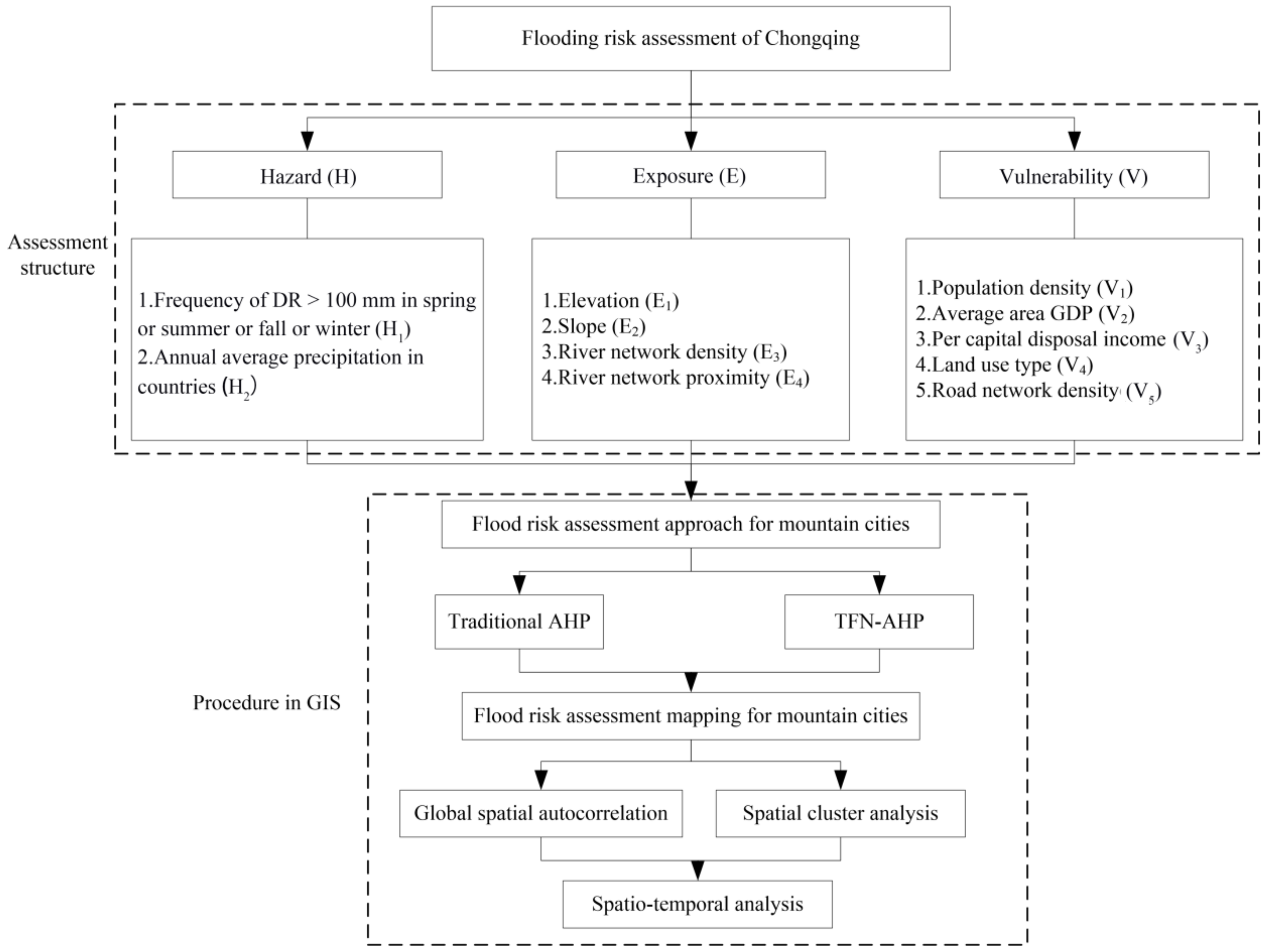
2.2. Research Framework

The flowchart of the flood risk assessment for Chongqing in this paper is depicted in three stages (Figure 2): (1) multi-indexes determination, (2) flood risk assessment experiments based on AHP and TFN-AHP methods and (3) flood risk spatio-temporal pattern analysis using GIS.

2.3. Flood Risk Assessment Method

2.3.1. Analytical Hierarchy Process (AHP)

The AHP separates a complicated issue to a form an object layer, index layer and sub-index layer. In this field, the object layer is used to represent the risk, and the other layers consist of detailed assessment indicators. According to the Analytic Hierarchy Process proposed by Lin, Kairong, et al. [13], integer numbers of 1–9 compose pairwise comparative scales. Number 1 refers to identical significance between index A and B, and number 9 means A outweighs B significantly for the risk. The consistent judgment matrix can be constructed after determining the importance of assessment indexes. Ultimately, based on the largest eigenvalue, vectors are calculated for consistency verification using Equations (1)–(3):
λ max = i = 1 n A w i n w i
C . I = λ max n n 1
C . R = C . I R . I
where λ max is maximum eigenvalue, (Aw)i is the ith factor of (Aw) of the vector, C.I is the consistency index and R.I is the random consistency index. If the C.R value is less than or equal to 0.1, it demonstrates that the matrix meets the verification conditions. Otherwise, the scale values of i and j need to be reassigned to check the matrix.

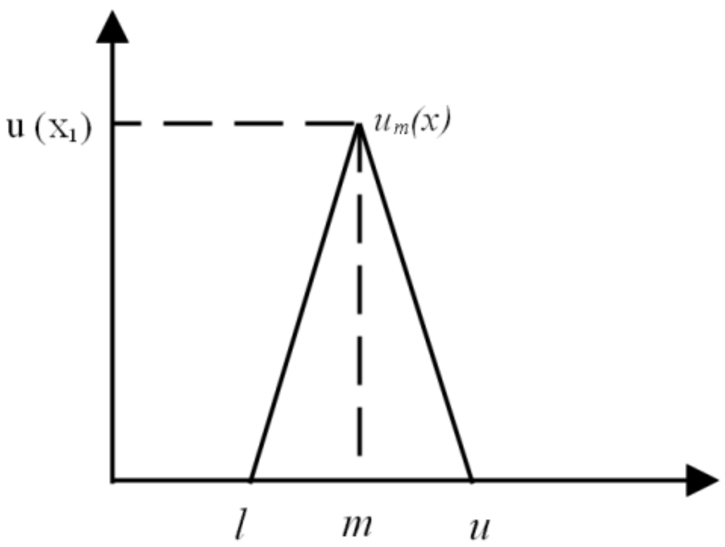
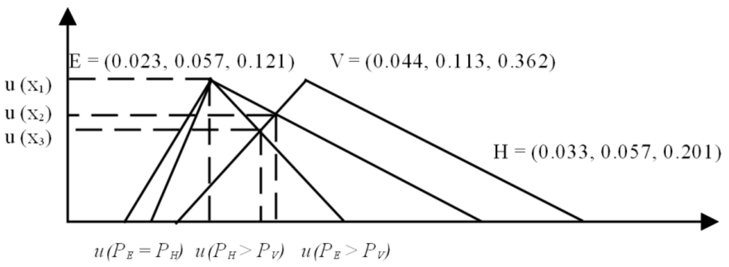
2.3.2. Triangular Fuzzy Number-Based Analytical Hierarchy Process (TFN-AHP)

The TFN-AHP is the combination of the original AHP and triangular fuzzy numbers. The traditional AHP is often represented as the importance degree between factors by crisp numbers, while this method uses triangular fuzzy numbers instead. That is to say, using the expression of a triangular fuzzy number, P = (l, m, μ), to replace a crisp number with others remaining unchanged, where l, m and μ are the minimal, most probable and maximum risk value, respectively. The key of the approach is using l and μ to measure the value of m, depicted in Figure 3 according to its principals [37]. In this way, TFN-AHP determines the probable importance degree between two numbers regarding their influences on flood risk, rather than definite degree of crisp numbers. Then, the extended value range of importance degree increases the accuracy of the weights of assessment factors. Table 2 demonstrates the meaning of triangular fuzzy numbers, which stands for their importance in flood risk assessment. For instance, the number 1 in the comparison result of H1 and H2 means that the two indicators have the same impact on flood risk. If the number is 7, it means that H1 exerts a significantly greater impact on flood risk than that of H2. The relationship of two triangular fuzzy numbers is calculated through TFN-AHP. The detailed theory can be found in [24].

2.3.3. Incorporation of AHP and TFN-AHP into GIS

Flooding is the consequence of comprehensive effects of hazard, exposure and vulnerability. Each index contains several risk indicators, and the expression of flood risk is defined as Equation (4):
F R = w H i = 1 n w i H i + w E j = 1 n w j E j + w v k = 1 n w k V k
where wH, wE and wV are the weights of hazard, exposure and vulnerability respectively, wi, wj and wk are the weights of each factor and Hi, Ej and Vk are the normalized indicators. Based on weights from AHP and TFN-AHP of input GIS 10.2, Equation (4) is calculated using the fuzzy classification function in GIS to obtain flood risk.

2.4. Assessment Indexes

As shown in the flowchart of Figure 2, the flood risk is defined as hazard, exposure and vulnerability, according to the fifth appraisal report of the Intergovernmental Panel on Climate Change (IPCC). Thus, a flood risk assessment model was established on the basis of the principal of AHP, consisting of an object layer, an index layer and a sub-index layer [38]. There are diverse factors in each layer, weights of which were calculated using AHP and TFN-AHP, and then processed in GIS. Many indicators can contribute to flooding increase. Based on literature reviews, eleven flooding influencing factors were selected to investigate floodplains, which are average annual precipitation, average daily rainfall, elevation, slope, river network proximity, river network density, population density, average area GDP, per capital disposable income, road network density and land use type.

2.4.1. Hazard Index

Here, hazard chiefly refers to meteorological factors such as typhoons and rainstorm [39]. As an inland city, rainstorm is the primary meteorological index triggering floods in Chongqing. The average annual precipitation in each county reflects the precipitation intensity of the current year. The frequency of rainstorm, the average daily rainfall exceeding 50 mm, is the source of floods. This paper adopts the above two meteorological indicators, frequency of rainstorm (H1) and average annual precipitation of counties (H2), to measure the hazard of flooding, which can be expressed as:
H = w H i = 1 n w i H i
The above data can be processed by Kriging interpolation in GIS to prepare precipitation maps, and the concrete information can be found in [24].

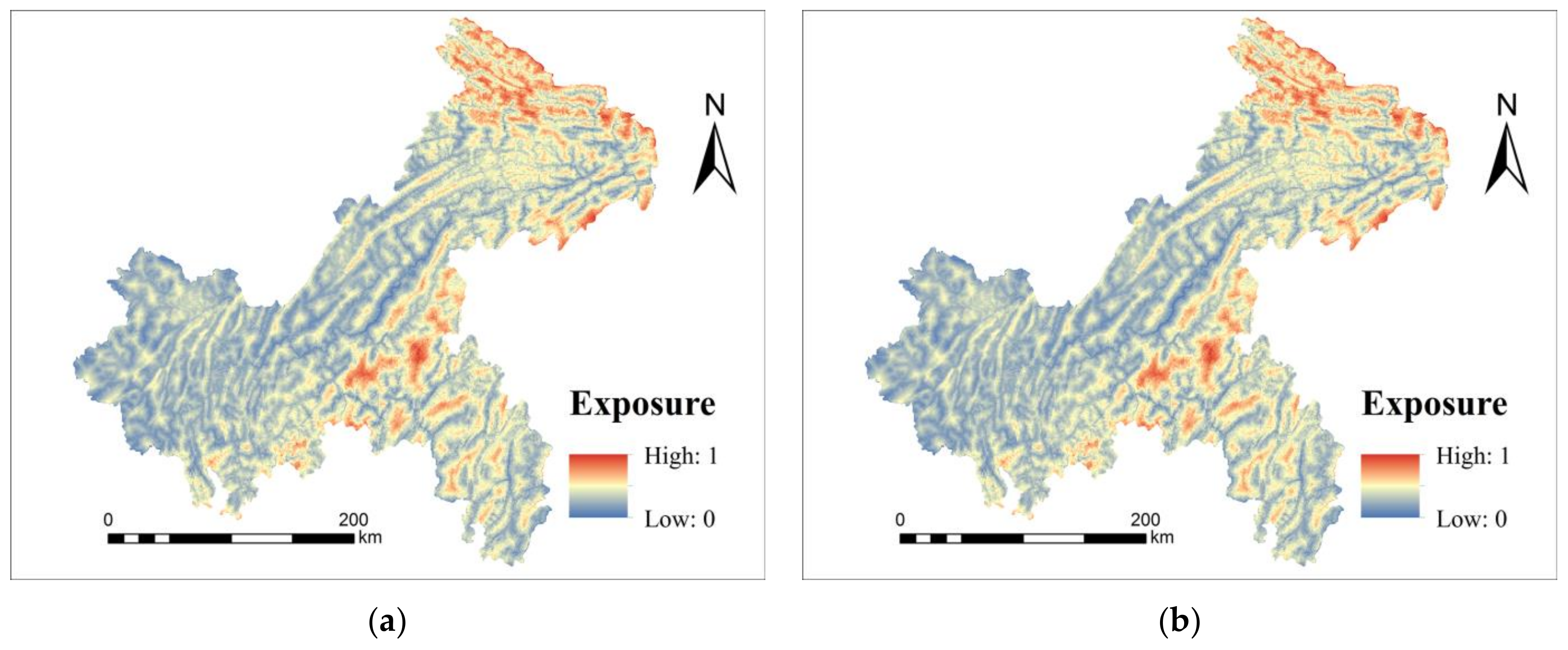
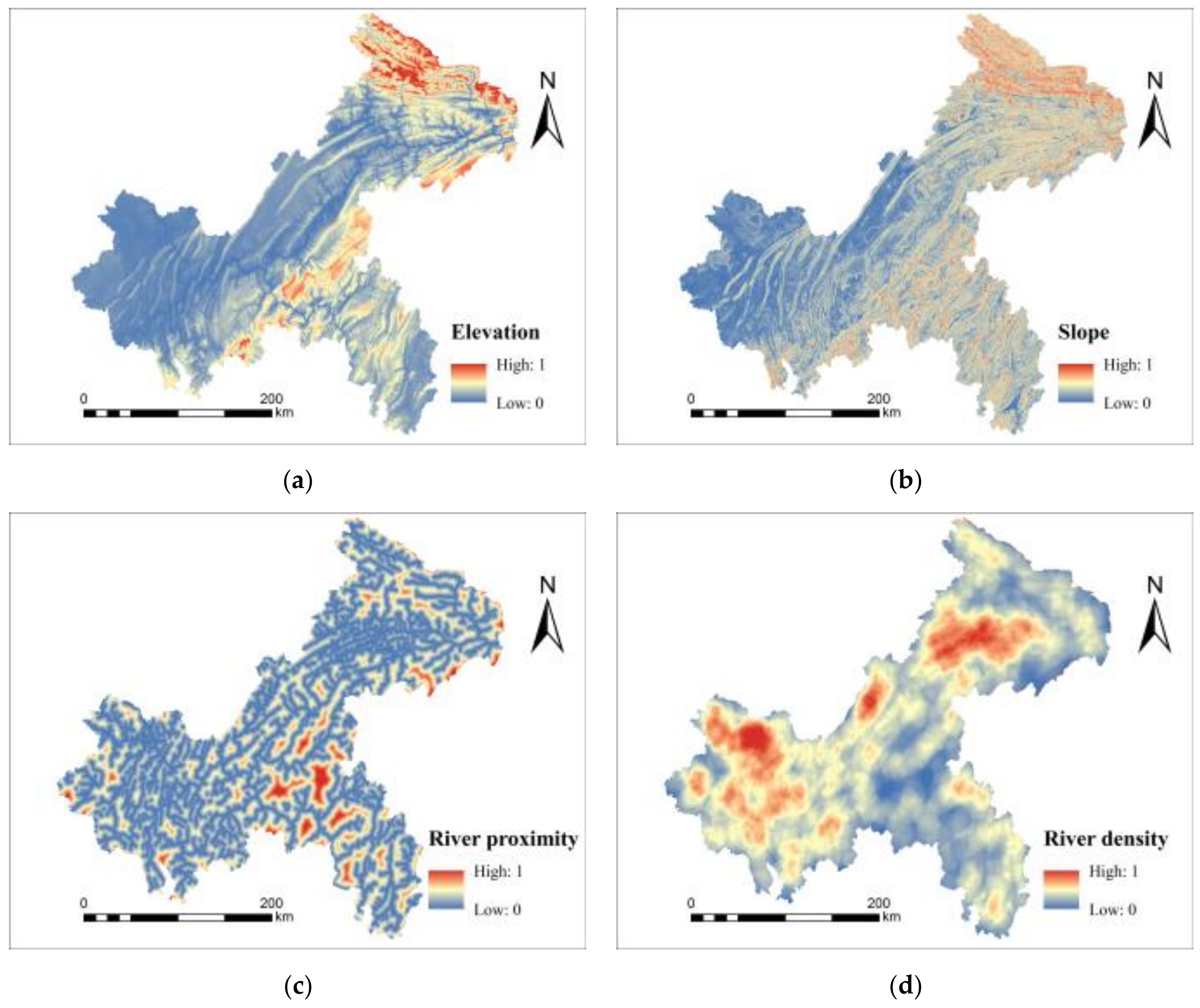
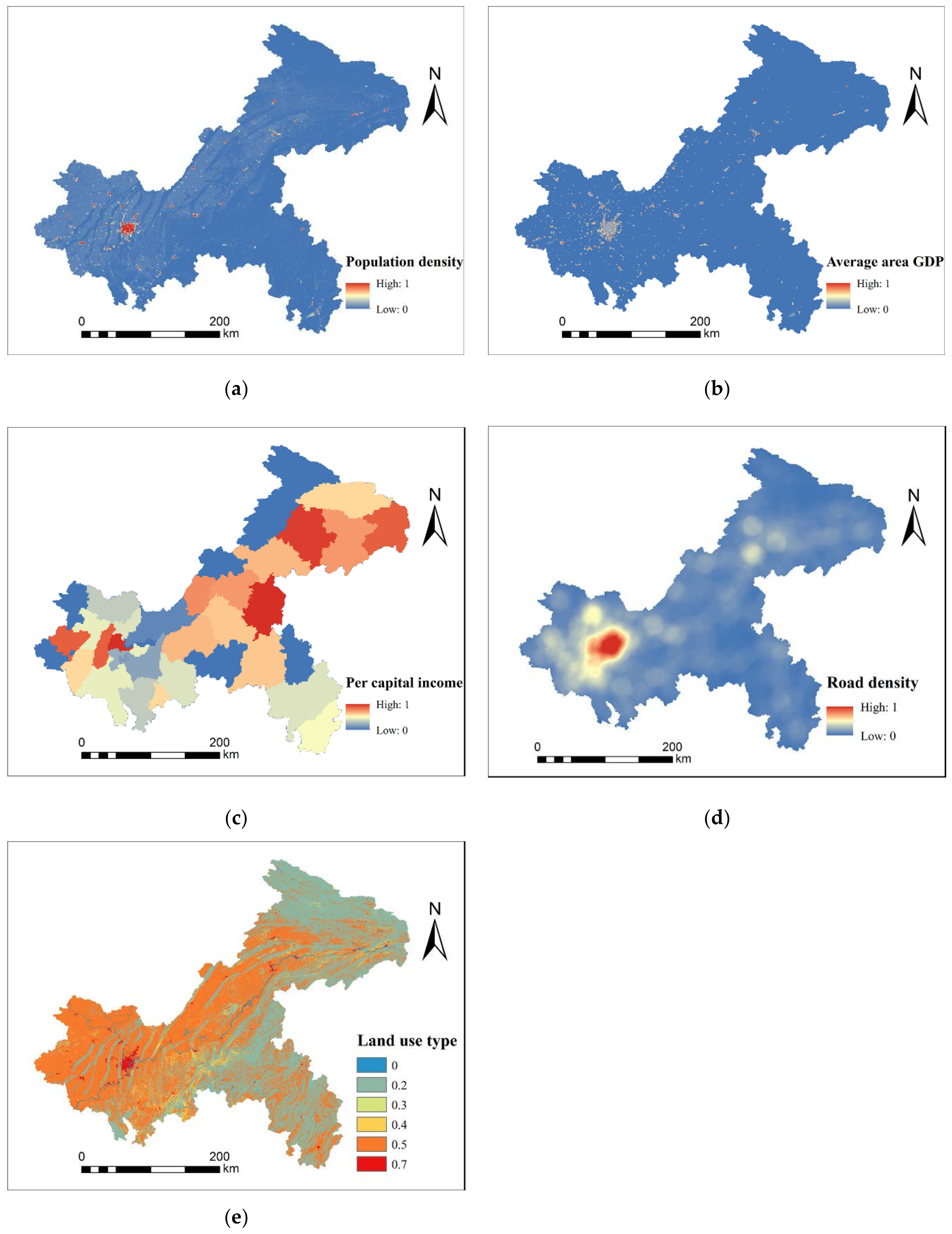
2.4.2. Exposure Index

The exposure aspect contains elevation (E1), slope (E2), river network proximity (E3) and river network density (E4), expressed in Equation (6). Elevation and steeper slope indicate a topographic impact on flooding. We use river network proximity and its density to speculate river conditions, since river existence is one genesis of flooding.
E = w E j = 1 n w j E j
The elevation and slope are extracted using the surface analysis of 3D Analyst. Euclidean distance is applied to prepare the river proximity layer. The river network density is the ratio of the average river length to the average adjacent area, which can be acquired through linear density. The basic theory is expressed as:
D i = R i j A i
in which Di, Ai and Rij are the river density, the area and the length of the jth river of the ith pixel, respectively.

2.4.3. Vulnerability Index

As for vulnerability, the resistance of disasters, in Equation (8), we choose population density (V1), average area GDP (V2), per capital disposable income (V3), road network density (V4) and land use type (V5) as assessment indicators. The influence of floods on people’s lives is examined by population density. The average area GDP, per capita disposable income and road network density are representatives of asset vulnerability and recovery capability. The impact on local agriculture is identified by land-use type.
V = w v k = 1 n w k V k
The expression of road network density is similar to the formula of river network density.
After the above data processing, risk raster format maps with a pixel size of 98 × 98 were obtained using Raster Calculation of GIS. However, as all indicators have different dimensions, it is necessary to normalize them for uniform comparisons. Thereby, the value needs to be converted into a unified [0, 1] range by the fuzzy classification in the GIS. In the model, the assessment indexes have been divided into positive and negative factors (Equations (9) and (10)), as they have adverse impacts on flood risk:
x = m i m max m max m min
x = m max m i m max m min
where x is the normalized value, mmax and mmin are the maximum and minimum values respectively, and mi is the original value.

2.5. Weight Calibration

2.5.1. AHP Weight

The judgment matrix of the index layer was obtained on the foundation of pairwise comparison, as demonstrated in Equation (11). Based on the Equations (1)–(3), the consistency ratio of judgment matrix, Findex, was determined as 0.008, which was less than 0.1, so the consistency of the judgment matrixes was satisfied. Similarly, the weights of sub-index layers can be calibrated, as tabulated in Table 3.
F i n d e x = H E V H 1 3 2 E 1 / 3 1 1 / 2 V 1 / 2 2 1

2.5.2. FN-AHP Weight

The consistent judgment matrixes of AHP can be substituted by triangular fuzzy numbers to gain the fuzzy judgment matrix of each layer. The weight calibration process of TFN-AHP is illustrated using the judgment matrix of the index layer as an example. According to the fuzzy judgment matrix of the index layer listed in Table 3, the fuzzy synthetic extent (Pi) was calculated, which is drawn as triangles in Figure 4. Based on that, the triangular fuzzy affiliation of the index layer was obtained.
The affiliation of hazard and exposure was computed as follows:
μ   P H   P E = 1 ,   μ   P E P H   =   1
The affiliation of exposure and vulnerability was calibrated as follows:
μ   P E P V = 0.512 ,   μ   P V P E   =   1
The affiliation of hazard and vulnerability was reckoned as follows:
μ   P H   P V = 0.690 ,   μ   P V P H   =   1
According to TFN-AHP theory, the original weight of each factor was calibrated: W0 = (1, 0.512, 0.690).
After standardization, the weights of the index layer were: Wb = (0.454, 0.313, 0.233).
As the triangular fuzzy judgment matrix of the hazard, exposure and vulnerability indexes given in Table 4, Table 5, Table 6 and Table 7, similarly, the weight of each sub-index layer can be computed following the above procedure.

2.6. Spatio-Temporal Analysis Method

The overall spatial autocorrelation of regional risk is regularly measured by Global Moran’s I index, due to its simple operation and judgment ability. In detail, this method can judge whether there is agglomeration or outlier, which can be used as the basis for further analysis of spatial autocorrelation distribution. Its value, ranging from −1 to 1, is an inferential reflection of negative and positive spatial correlation, respectively [27]:
I   =   i 1 , j 1 n W i j ( x i x ) ( x j x ) i = 1 n ( x i x ¯ ) 2 / n i 1 , j 1 n W i j
where n represents the total number of spatial units, x is the inundation risk of unit, i and j are the candidate unit and neighboring unit, x ¯ is the average value of the flood risk of all units and Wij denotes the spatial weight matrix.
Global spatial correlations are not consistent with local clustering, and they are two spatial autocorrelation analysis methods from global and local aspects. Thus, Anselin Local Moran’s I is adopted to evaluate the spatial clustering types between spatial units. The formula is expressed as follows [40]:
I i   =   x i x ¯ i = 1 n ( x i x ¯ ) 2 / n 1 i 1 , j i n W i j ( x i x ¯ )
in which x, x ¯ and Wij are the same as in Equation (15).

3. Results

3.1. Comparative Analysis of Flood Risk of AHP and TFN-AHP Methods

After the data processing according to Section 2.4, including standardization and weights calculation, all sub-indexes were overlaid through the Raster Calculator of GIS. Then, based on the Equations (4)–(8), AHP and TFN-AHP approaches were used to map the index layers, hazard, exposure and vulnerability. This work uses fuzzy terms of high and low to represent the level of risk, rather than accurate classification.

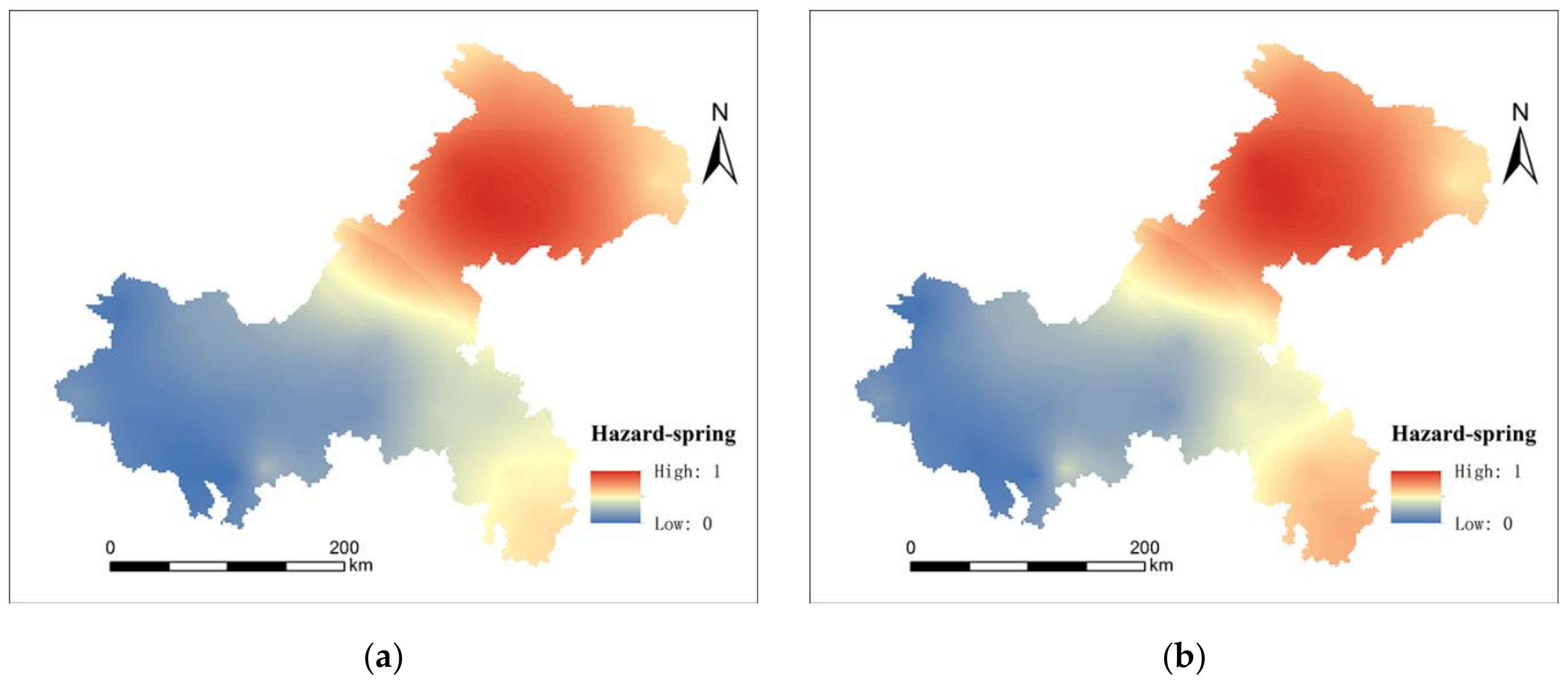
3.1.1. Hazard Results

It is well-known that rainfall varies from one year to another. Compared to the annual precipitation of 2000 to 2018 in Chongqing, the precipitation in 2018 was higher than before 2014. Considering data availability, daily precipitation of 2018 was chosen as the hazard sub-index, which is representative rather than haphazard. Subsequently, according to the weights listed in Table 3 and Equation (1), the spatial distribution maps of hazard in Chongqing from the two methods were obtained, as shown in Figure 5. Visually, the results of the two approaches are dissimilar in four seasons. That is to say that their maps during spring and autumn have almost identical trends, and consequences from TFN-AHP are less hazardous than AHP in summer and winter, especially in the central area. This is likely on account of the comparison where TFN-AHP determined lower weight of daily precipitation and higher weight of annual precipitation than those from AHP. For the same precipitation data, in the summer season with high daily precipitation, the larger the weight of daily precipitation is, the greater its impact on hazard. The difference of winter precipitation remains to be explored, while the difference between the two weights will be relatively small in seasons with little daily precipitation. Consequently, results from the two methods in spring and autumn represent no abrupt difference, and the variation of the weight of H1 is expanded in summer and winter, leading to distribution divergence.
Floods are not only determined by the precipitation of a season, but also closely related to the precipitation of the whole year. This is because precipitation is generally cyclical. The precipitation decreases from northeast to west in spring, from southeast to north in summer and from west to east in autumn and winter. The precipitation in one season may change in its cycle due to climate change, which may lead to the advancement or delay of the rainy season, which may affect the precipitation in other seasons [41]. The annual precipitation is used as an auxiliary evaluation factor, in order to decrease the possibility of this phenomenon. Thus, TFN-AHP can improve the accuracy of the results by increasing the weight of annual precipitation.

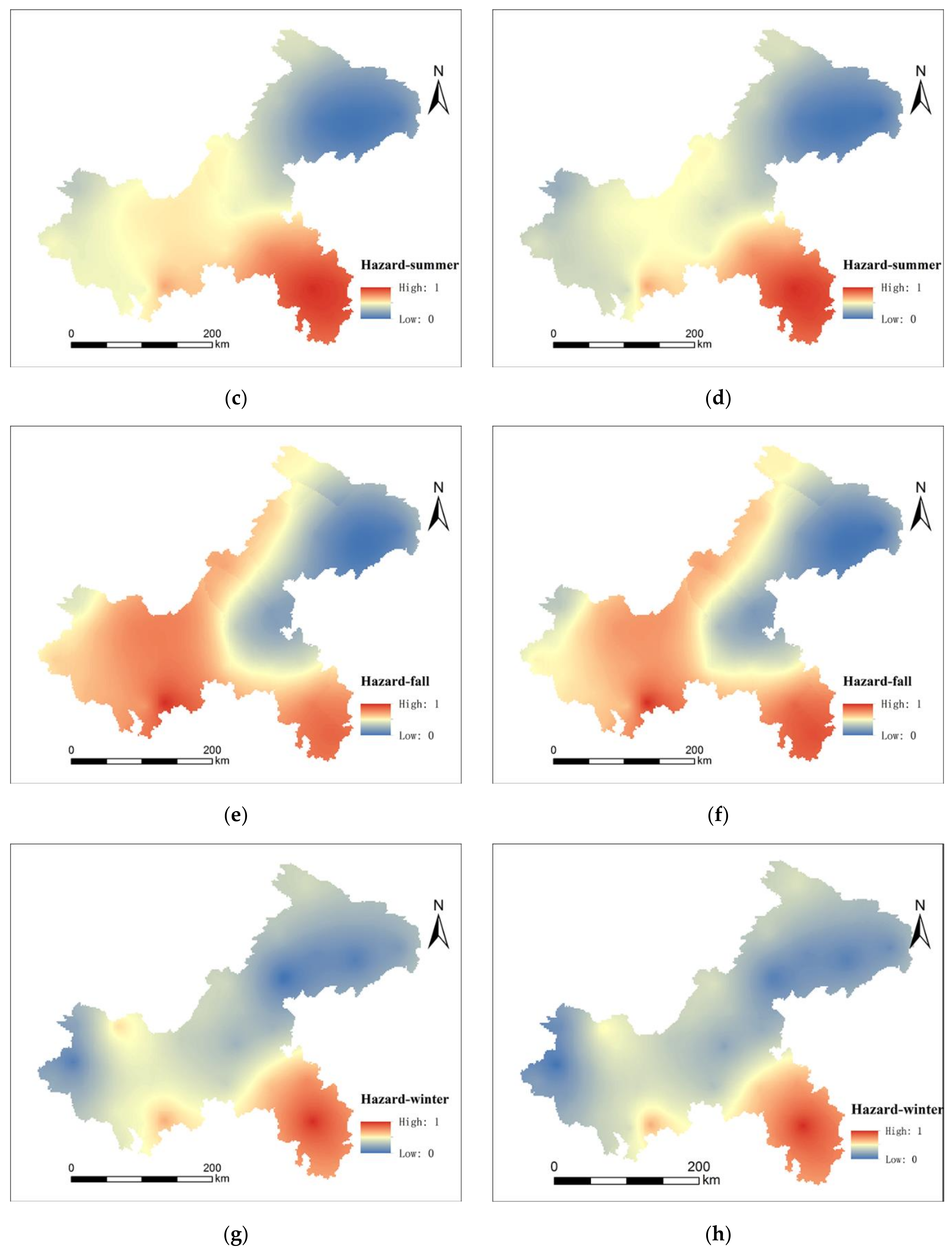
3.1.2. Exposure Results

With respect to exposure, the weights followed in Table 3 and Equation (2) were combined to map the spatial distribution of exposure using the above two methods, as shown in Figure 6. It should be noted that exposure indexes are negative indicators, manifesting that the lower value of which stands for the higher exposure. A clear divergence of consequences from the two approaches is visible in that the result from AHP is more exposed than that from TFN-AHP, owing to the higher weight of H3 from TFN-AHP. The integrated effect of increased weights of negative factors and negative value minimizes the overall exposure, just like maps of TFN-AHP.
The effectiveness of the two approaches can be explained from two perspectives. First, in the typical mountain city Chongqing, elevation and slope are the main differences, as well as the key factors affecting floods in different districts. Comparing the Figure 6 and elevation and slope in Figure 7, we can easily find that their trends are very similar. The northeast and southeast have higher altitude and larger slope, which is due to the Daba Mountain in the north, Wushan mountain in the East and Wuling Mountain in the southeast. Whereas the sum weights of elevation and slope from TFN-AHP are greater than those from AHP, resulting in the trend of exposure from TFN-AHP relatively similar to that of elevation and slope maps in Figure 7. Secondly, the counties closer to the river are inclined to trigger water levels rising to flooding level, without which, there will be no flooding no matter how dense the river network. Since rivers flow through almost all districts in Chongqing (Figure 7), such as Yangtze River running through the city, Jialing River and Wujiang River, and so forth, the influence of H4 should be minimized. Thereby, the weight of H3 is enhanced to stand out as important. In summary, the impact of elevation and river network proximity can be more accurate and match well with the actual situation using TFN-AHP.

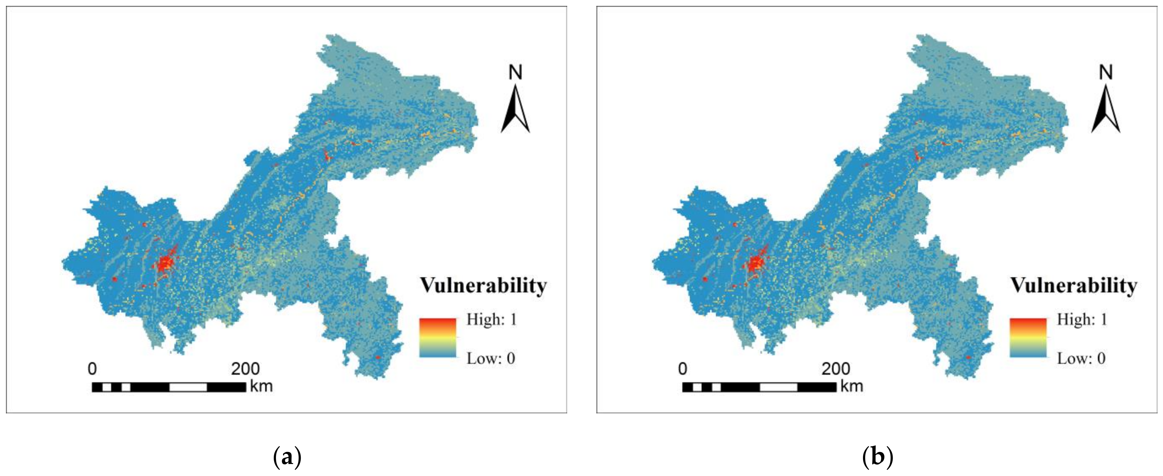
3.1.3. Vulnerability Results

In view of vulnerability, according to references [42,43] and the Delphi method, the vulnerability values of each land use were obtained through scoring 0–1 to the vulnerability of land use types. The thresholds in Figure 8e are the average value of vulnerability to flood risk of each land use. Then, integrated with the weights in Table 3 and Equation (3), the spatial distribution maps of rainstorm vulnerability from two approaches are presented in Figure 9. The vulnerability results from the two approaches follow the same distribution. These are understandable from two aspects. One is the impact of the identical weights of V1, V2 and V3. Just as a multitude of works assert, economy and population are closely related to disaster resistance. This is due to the fact that the economy is the sign of detailed planning of preventive measures, multi-fund recovery and reconstruction, and people are the primary disaster-bearing body. Hence, consequences of either approach will follow the trend of the three factors in the Midwest, remaining high in V1, V2 and V3 indexes and vulnerability, as shown in Figure 8 and Figure 9. The other is that, though weights from the two approaches of V4 and V5 are varied, the sum accounts for a small proportion compared to other indicators. Thus, the variation imposes a slight impact on vulnerability. However, the lower weight of V4 from TFN-AHP is noteworthy. For Chongqing, with much area with a less dense road network, V4 should weaken its proportion to minimize the role of road network and make the weight structure more reliable. Thereby, weight determination is handled better with the use of TFN-AHP, especially for V4.

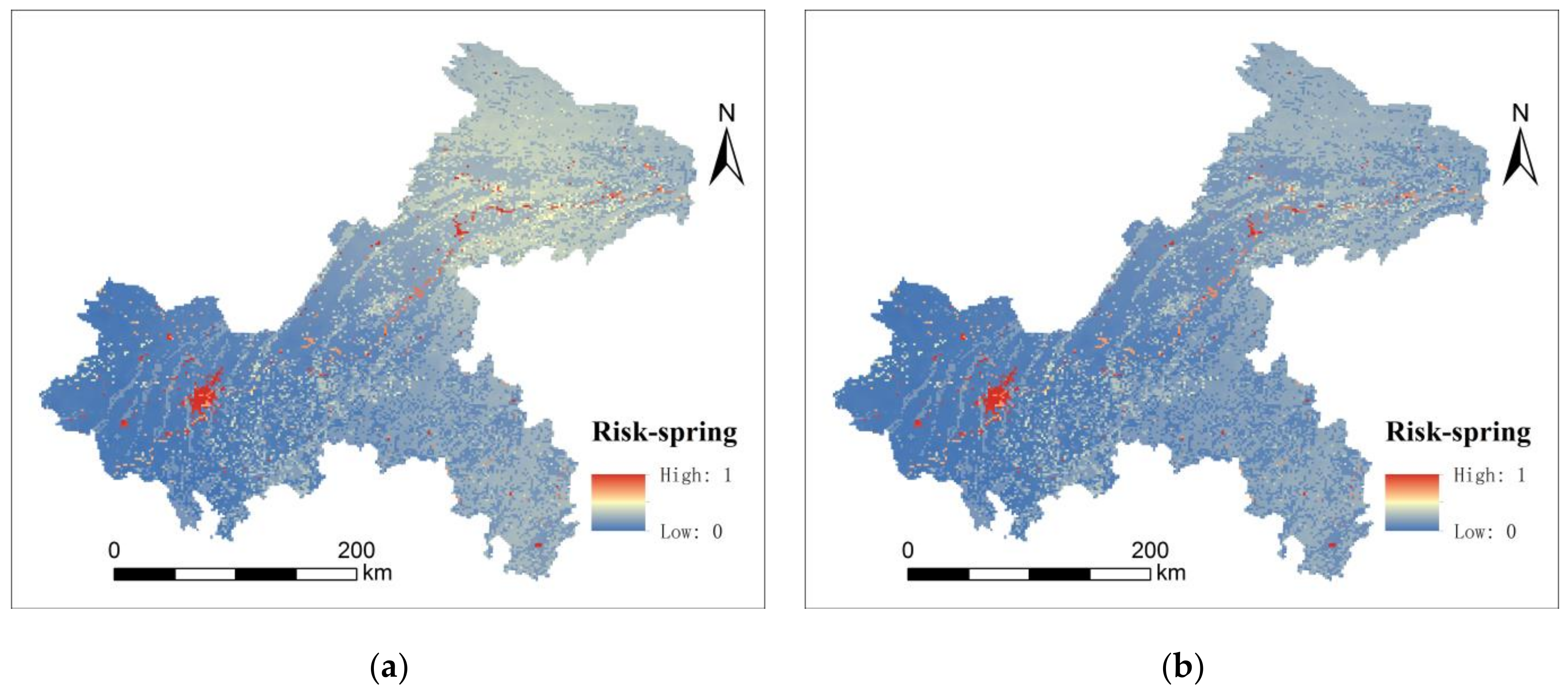
3.1.4. Flood Risk Results

The above index-layer consequences were weighted and integrated to obtain the comprehensive risk of floods, as shown in Figure 10. Visually, the main difference is that the risk of AHP in the northeast and southeast is higher than that of TFN-AHP. Two reasons are responsible for this phenomenon. First, considering the aforementioned analysis, the exposure of TFN-AHP is lower than that of AHP, reducing the risk of areas corresponding to the lower value in the exposure map from TFN-AHP, and the difference of flood risk is mostly distributed in the northeast and southeast, which is the same as exposure maps. Additionally, the exposure and vulnerability estimated by TFN-AHP have comparably greater weights by comparison of the two methods. The increased exposure weight multiplies the lower value, which brought about a drop of risk level derived from TFN-AHP. The flooding statistics of 2018 demonstrated that the southeast, such as Xiukou county, underwent few flooding disasters, and the zones evaluated by TFN-AHP are observed to be lower risk compared with those by AHP, indicating that TFN-AHP performs better in flooding risk assessment. Therefore, TFN-AHP is employed in the work.

3.2. Temporal-Spatial Analysis of Flooding Risk

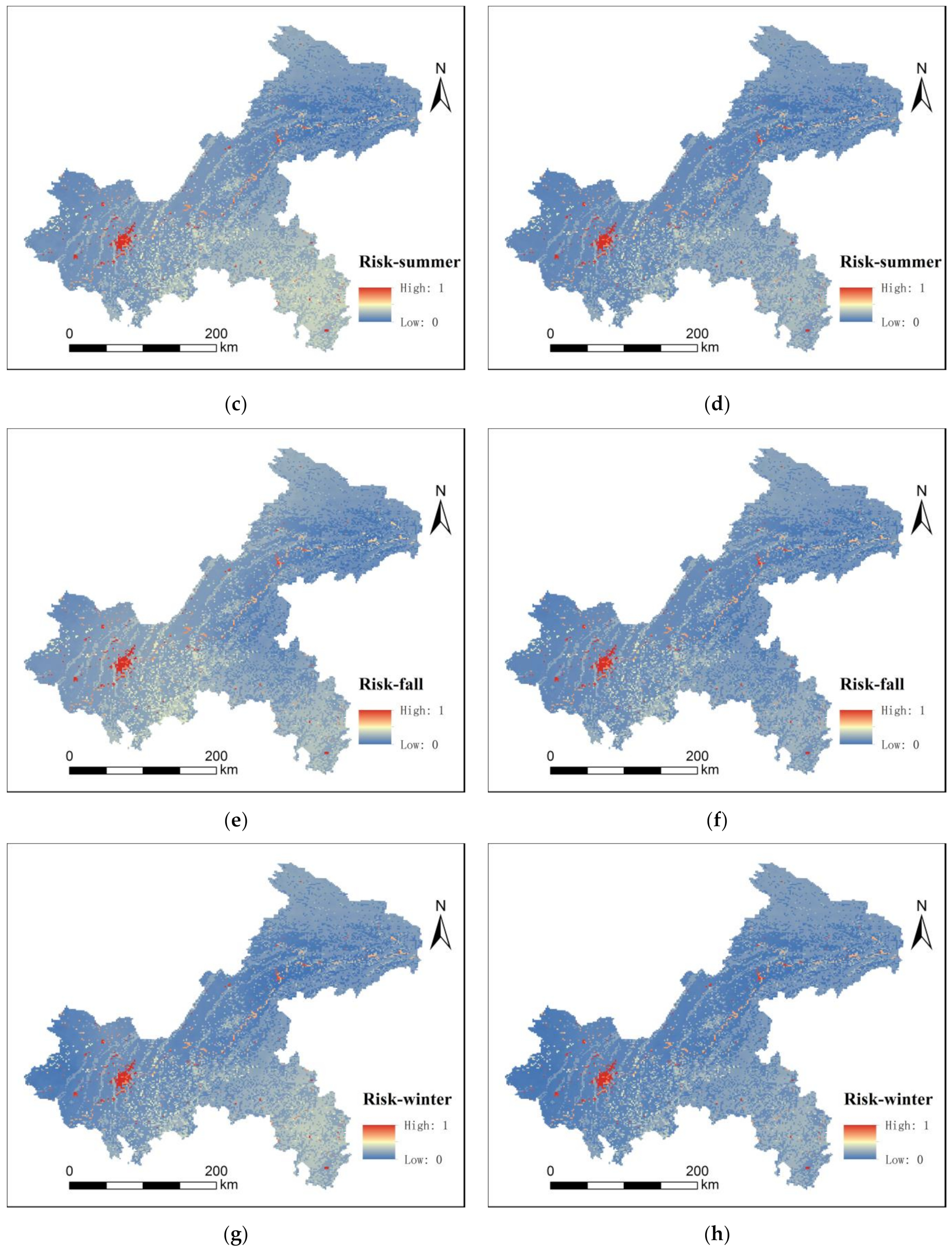
3.2.1. Seasonal Difference of Flooding Risk

Notably, as shown in Figure 10, the differences in four seasons lie in low–medium-risk areas, distributed over most parts of Chongqing. This can be interpreted by the role of hazard factors. To be clear, frequency of precipitation, the decisive hazard factor, experiences dramatic changes in diverse seasons. In all seasons, the comprehensive effects of high exposure and high vulnerability are attributed to urban areas and the areas along the Yangtze River, assessed as the most-risky locations.

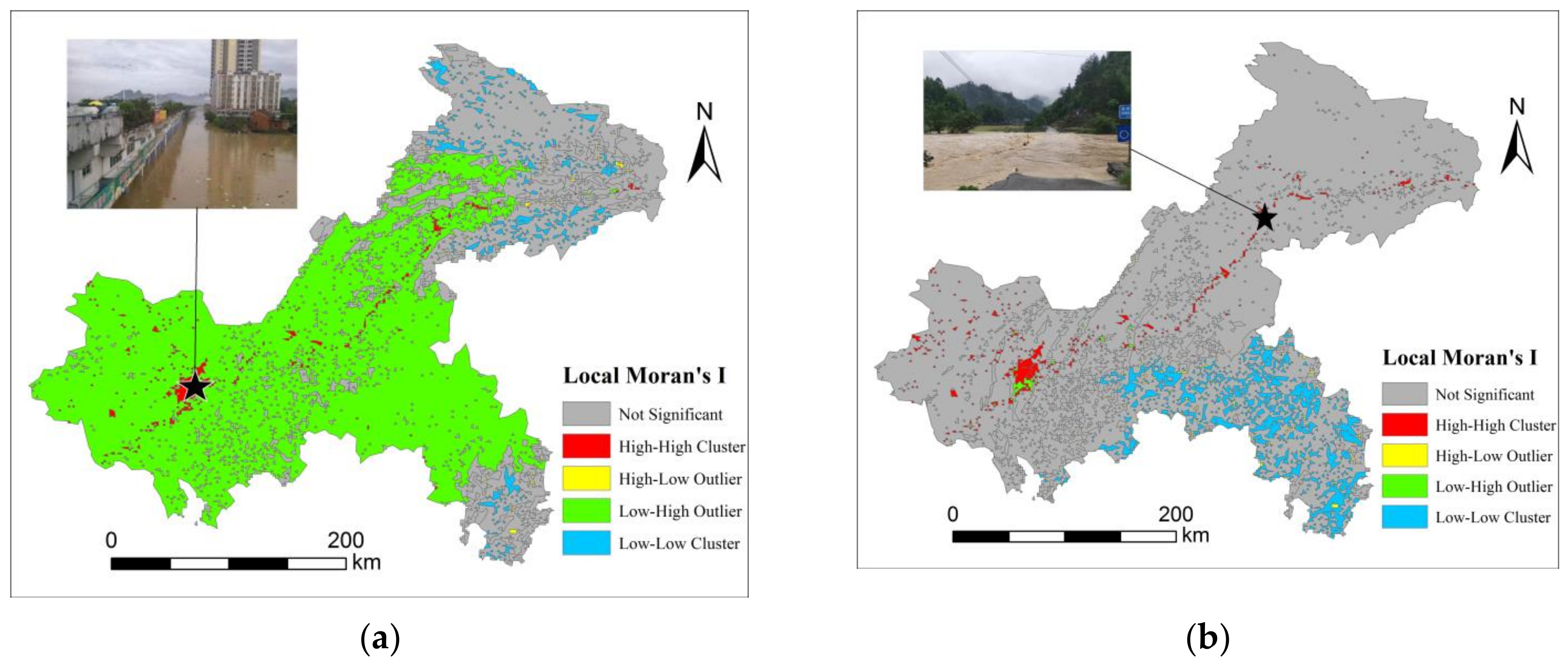
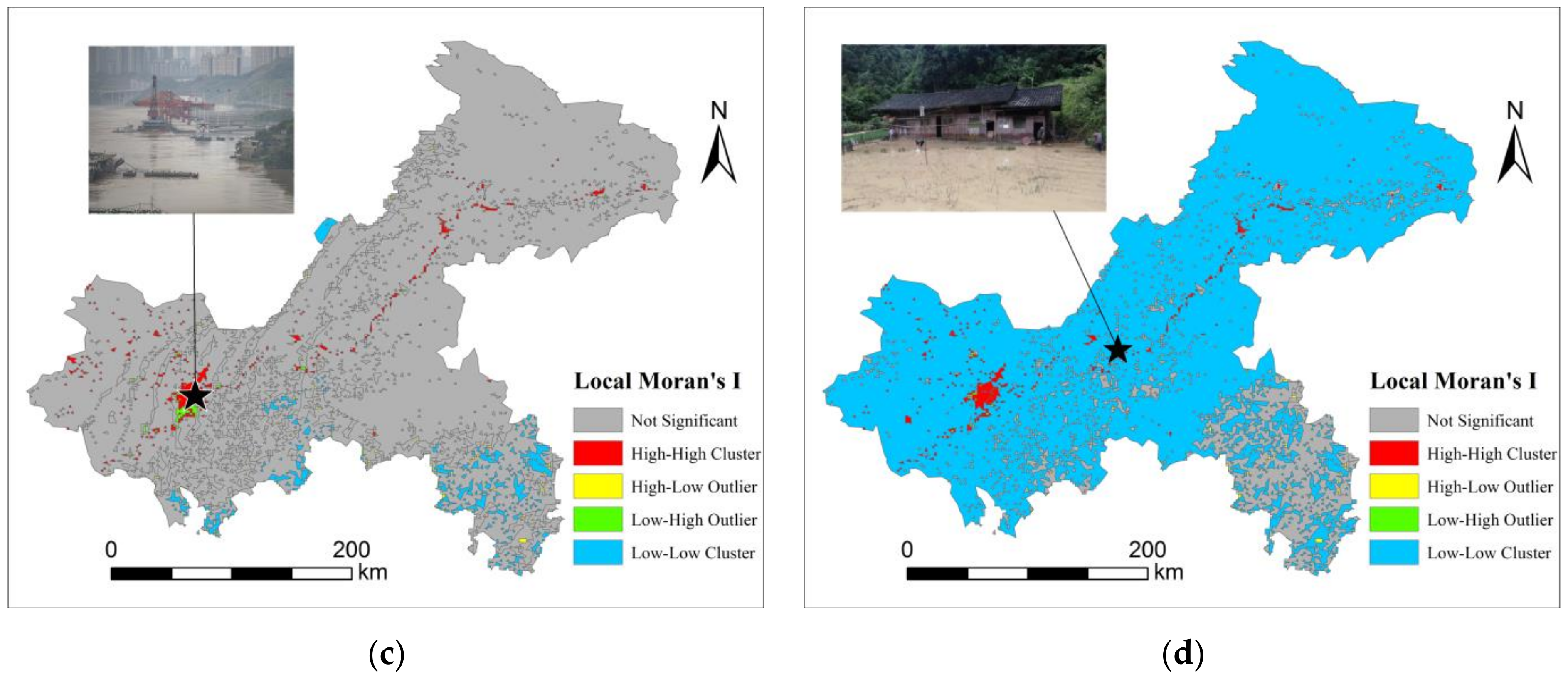
3.2.2. Spatial Analysis of Flooding Risk

Based on the spatial technology in ArcGIS, the Global Moran’s I, Anselin Local Moran’s I and the corresponding Z and P value of Chongqing’s flood risk were obtained as presented in Table 8. Z(I) is greater than 1.96 and P is less than 0.05, both satisfying the critical value of normal distribution function at the 0.05 level. As such, the global autocorrelation outcomes can be thought of as significant. Moreover, Anselin Local Moran’s I is a requisite for further spatial clustering exploration under three considerations, hazard, exposure and vulnerability.
It can be seen from Figure 11 that the distributions in four seasons are identical in high-high clusters (HH). To be precise, the main urban area and areas along the Yangtze River are outstanding as HH spots. It is critical to note that the exposure and vulnerability of these zones are the highest, which are the main leading factors of hot spots. In detail, as shown in Figure 11a, the main urban area has a high vulnerability due to advanced economy as a flooding-bearing body. Along the Yangtze River area is sensitive to the high exposure brought by river surge and low-lying areas (Figure 11b,c). It is easy from Figure 11d to observe that some hot spots in southeast and mid zones are under the effect of poor finance development, since their location is surrounded by mountains. In regard to the differences of four seasons, most areas are low-high clusters (LH) in spring, not significant clusters in summer and autumn and basically low-low clusters (LL) in winter. This suggests that high-risk zones lack early warning and post-disaster reconstruction capabilities and flooding control policies need to change from season to season.

3.2.3. Temporal-Spatial Analysis of Flooding Risk

According to the above analysis on the basis of data from 2018, it is easy to find the changing and constant zones in all seasons of 2018, as seen in Figure 11. Overall, regions changing with seasons are distributed in west and central zones. The results show that they tend to be lower risk from spring to fall, with risk increasing in winter. It is evident that hazard indicators play a critical role, since the distributions of exposure and vulnerability are similar in these regions. In detail, the cold air masses of spring, together with the rainy season in summer and autumn, lead to an increase of LL clusters accompanied with decreasing HH clusters. In winter, there is a pronounced decrease in all clusters under the influence of the southeast monsoon. With regard to the constant parts, main urban areas and areas along the Yangtze River are always high-risk, with high values of both exposure and vulnerability, and the southeast region is LL clusters, as shown in Figure 11.

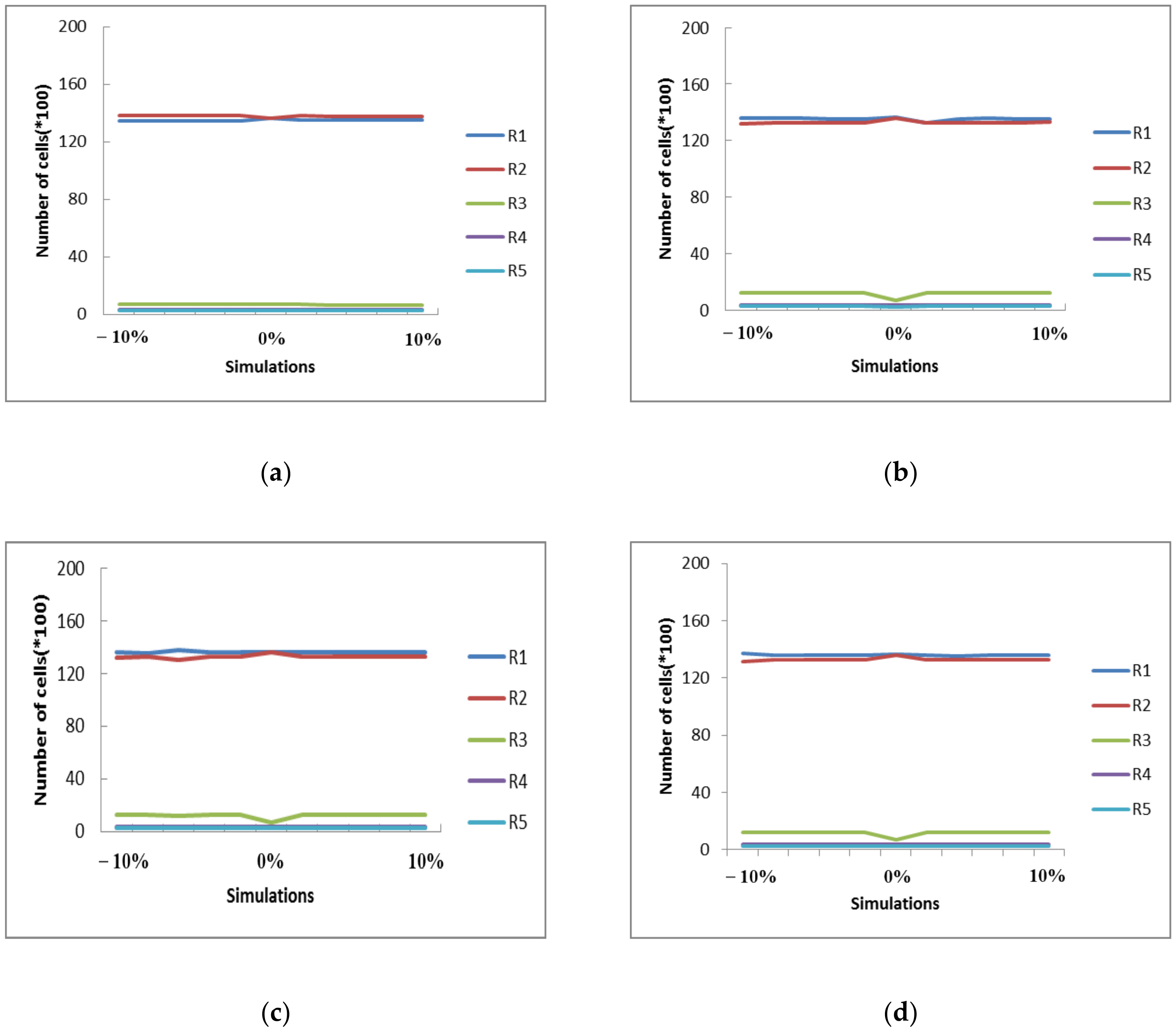
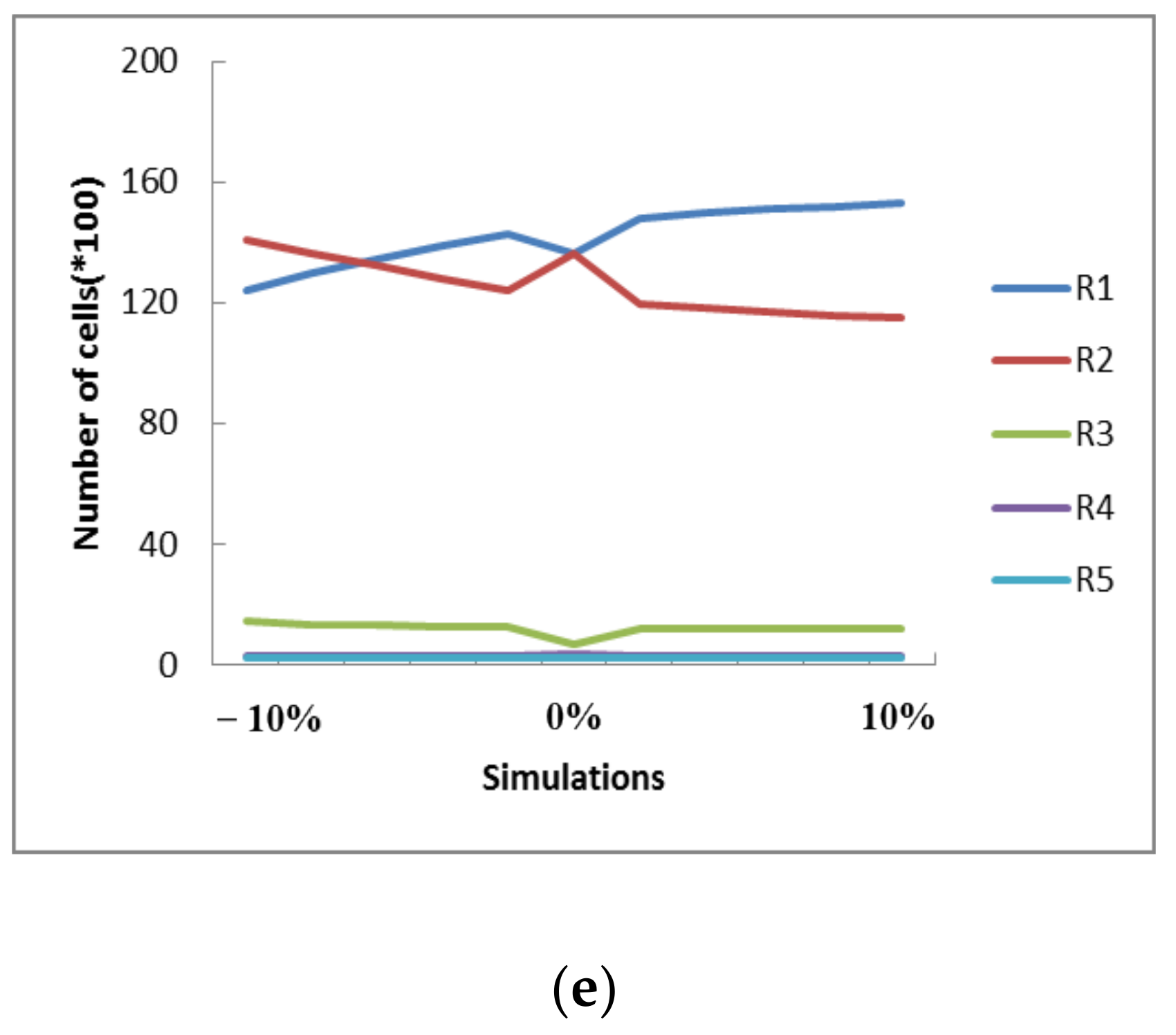
3.3. Sensitivity Analysis of Assessment Factors’ Weights

According to relevant references, the results are highly sensitive to the weights of assessment indicators. In this study, sensitivity analysis of assessment factors’ weights was performed. The approach changes the weights of one indicator and keeps other indicators fixed [44]. The range of weights’ deviations is set between −10% and +10% and the original weight is set as the baseline. Each time, the change is two percent. This study selected five indicators, which were H1, E2, E3, E4 and V4, covering almost all the weight values of different levels. According to the principle of sensitivity analysis, even if the weight of an indicator is altered, the sum weight of all indicators is always 1. Equation (14) is employed to adjust the weights of other fixed factors:
w i = ( 1 w m ) w i / ( 1 w m )
in which wm′ and wm are the changed and original weight of factor m, wi is the original weight of ith indicator and wi is the corresponding adjusted weight.
This work calculated 50 simulations and drew risk maps for each simulation. According to their standardized risk value, all maps were classified into five levels, very low risk, low risk, moderate risk, high risk and very high risk, as shown in Figure 12. The definitions of these five levels are demonstrated in Table 9. The results can be divided into three types based on the sensitivity. The first type is the most sensitive to weight alternation, such as V4. This type has a large fluctuation range in the whole range of change, for example, R1 shows an upward trend as a whole. The second type represents moderate sensitivity, just as E2, E3 and E4, which causes indispensable risk class modification when the alternation is −2% and +2%. Indicators such as H1 belong to the third type, with the lowest sensitivity. There exist hardly any fluctuations as the weights change in this type. This phenomenon demonstrates that indicators with lower weights are less sensitive, while indicators with heavier weights are more sensitive. This may be due to the fact that hazard has fewer indicators, and the overall indicator changes caused by weight changes are relatively small, whereas exposure and vulnerability consist of a large number of indicators. One factor change will cause other indicators to change, which will lead to a greater impact on the final result.

4. Discussion

4.1. Efficiency and Limitation

According to the assessment consequences, the urban areas and the Yangtze River coastal regions were evaluated as high-risk. In the process, the assessment indexes are the keys of risk. This work paid close attention to frequency of rainfall, river network density, elevation and population density, which are effective in flood risk prediction.
Frequency of rainfall is the determinate factor in flood occurrence. Without abundant precipitation, it is unlikely to result in flooding. Additionally, the weight of this index is 0.572, the largest value in all weights. By comparing the risk distribution map and hazard maps evaluated through rainfall data, the trends are identical. This shows that the zones with more rainfall are more prone to flooding. Observing Figure 5 and Figure 10, the urban regions and the Yangtze River coastal areas are at the highest risk, as well as having the most frequent rainfall. This is in line with the weights from TFN-AHP, which have been found in [45], which emphasized flood sensitivity to the rainfall. Therefore, choosing this factor can confirm reliable flood risk assessment results.
Investigating the influence of river network density and elevation on flooding risk showed that these two indicators affected the occurrence of flood the most. For one, it is well-known that river existence is one of the keys to floods. In addition, the weight of 0.332 suggests its unneglected influence on flood. Under the influence of the two reasons, the Yangtze River regions were taken as the highest risk, as demonstrated in Figure 10. For the other, the runoff discharge pattern may cause less flooding in areas with more rainfall, and relatively more floods in areas with less rainfall. For example, there are more heavy rains in hills and mountains than plains, and the elevation difference between mountains and hills aggravates the difficulty of stagnant water, making the probability of floods lower [46]. This reveals that elevation is the supplement to the rainfall factor, which can also be found through its weight of 0.318, ranking third in all weights. Thus, the stress on river network proximity and elevation can be proved using the high performance of these two indicators.
Since the higher the population density is, the more serious the flooding in the zone will be, there is a need to prevent the flooding through proper flood risk management. By TFN-AHP, a population with a weight of 0.3 is vital in flood occurrence. The relationship between population and flood risk can be seen using the results in Figure 8a and Figure 10, where the urban regions with high risk are populated places. So, the areas with more people are more sensitive to flooding risk.
From the above analysis, we can confirm that the assessment factors perform well in the prediction of flood risk. Then, an estimation of weight-determining methods verified the accuracy of the results. The statistics of flood disaster reports in each county during 2018 were collected from Chongqing Emergency Management Bureau. Based on that, the percentages of different risk levels of the two approaches and historical data were obtained, as shown in Figure 13. The highest zones of AHP and TFN-AHP are 0.01% and 0.008%, respectively. Besides, the higher regions of AHP and TFN-AHP are 0.01% and 0.02% respectively, and the highest and higher percentages of historical data are 0.02% and 0.13%. The comparison shows that TFN-AHP can yield more high-risk regions than AHP. Even though on account of limited data, the model and historical data are not exactly identical, the high-risk of all seasons from the model is relatively consistent with historical data. In conclusion, the adoption of TFN-AHP can provide more accurate insight into flood risk evaluation.
From the results of sensitivity analysis, it can be seen that the weights of various factors have different sensitivity, which highlights the importance of weight accuracy. For instance, with regard to the most sensitive factor, V4, its weight is reduced by 20%, which leads to a 33% change in the final result. Therefore, the accuracy of the weights plays an indispensable role in the accuracy of the evaluation results. The method of determining the weights with lower accuracy may have larger errors in the assessment results, thereby affecting the policies and decisions made by the decision-makers. Thus, the weights are necessary and crucial to increase the accuracy in the model. In this paper, TFN-AHP uses triangular fuzzy numbers to determine weights to reduce uncertainty. Its fundamental function is to employ fuzzy theory to gain better performance in accuracy enhancement, and the outcomes are consistent with the results of [24] and [25]. Although the TFN-AHP method is difficult to determine triangular fuzzy numbers, and this viewpoint is mainly subjective [47], the TFN-AHP approach is able to enhance the accuracy of flood risk assessment results, which is informative for decision-makers to efficiently manage flood risk.
The global regional risk pattern and local hot spots in Chongqing identified by GIS techniques are similar to historical floods, which can provide information for the government to formulate flood prevention and bank protection policies as a reference. Specifically, the global regional risk pattern can grasp the flood risk situation of the entire city as a whole, and hotspot risk areas can be employed as a supplement to focus on the prevention and control of flood, which is consistent with the flood control policy of the 14th Five-Year Plan formulated by Chongqing Municipality to focus on 298 key flood control risk points. The application of global regional risk pattern and local hot spots identification by GIS can be used in other mountain regions, such as Northern Fujian, mountain zones of Marginea and so forth. Then, this can better analyze the spatial distribution characteristics of floods in these mountain areas, and the visual advantage of GIS makes it easier to understand, thus creating more accurate flood control actions.

4.2. Reflections and Suggestions

In recent years, with the rapid development of social economy and the rapid promotion of the strategic position of Chongqing, flood risk management has become particularly important, calling for the development of specific policy measures. On the one hand, high-risk areas are principally distributed in the main urban areas and areas along the Yangtze River. For the main urban area, approaches such as planning drainage systems based on local conditions and promoting disaster data sharing and implementation of research achievements [48] are practicable and useful. For Yangtze River coastal areas, in addition to flood defense structures, the department should focus more attention on construction in flood-prone zones [49]. On the other hand, the southeast and northeast parts are low-risk areas. The power of the masses and specific environmental characteristics of mountain cities can be given full play in disaster prevention, because the utility of people and surroundings could benefit enhancing disaster-resilient capabilities [49]. Due to the different altitudes and socio-economic conditions of various mountain cities, the flood risk assessment results of Chongqing as an example are difficult to generalize to other mountainous cities. Nevertheless, the flood risk assessment indicators and methods used in this paper take into account some special topography and economic conditions of mountain cities and improve the universal applicability of the evaluation methods and indicators. Therefore, follow-up research needs to select the evaluation indicators as appropriate according to the local conditions and focus on methods and indicators that are generally applicable in all mountain cities.

5. Conclusions

The assessment method for mountain cities based on TFN-AHP and GIS was founded from three dimensions—hazard, exposure and vulnerability—in this paper to reduce the uncertain problem of risk assessment. For explicit flood risk management answers, the method provided vital insights into the risk level and temporal-spatial pattern. In general, the major conclusions are as follows:
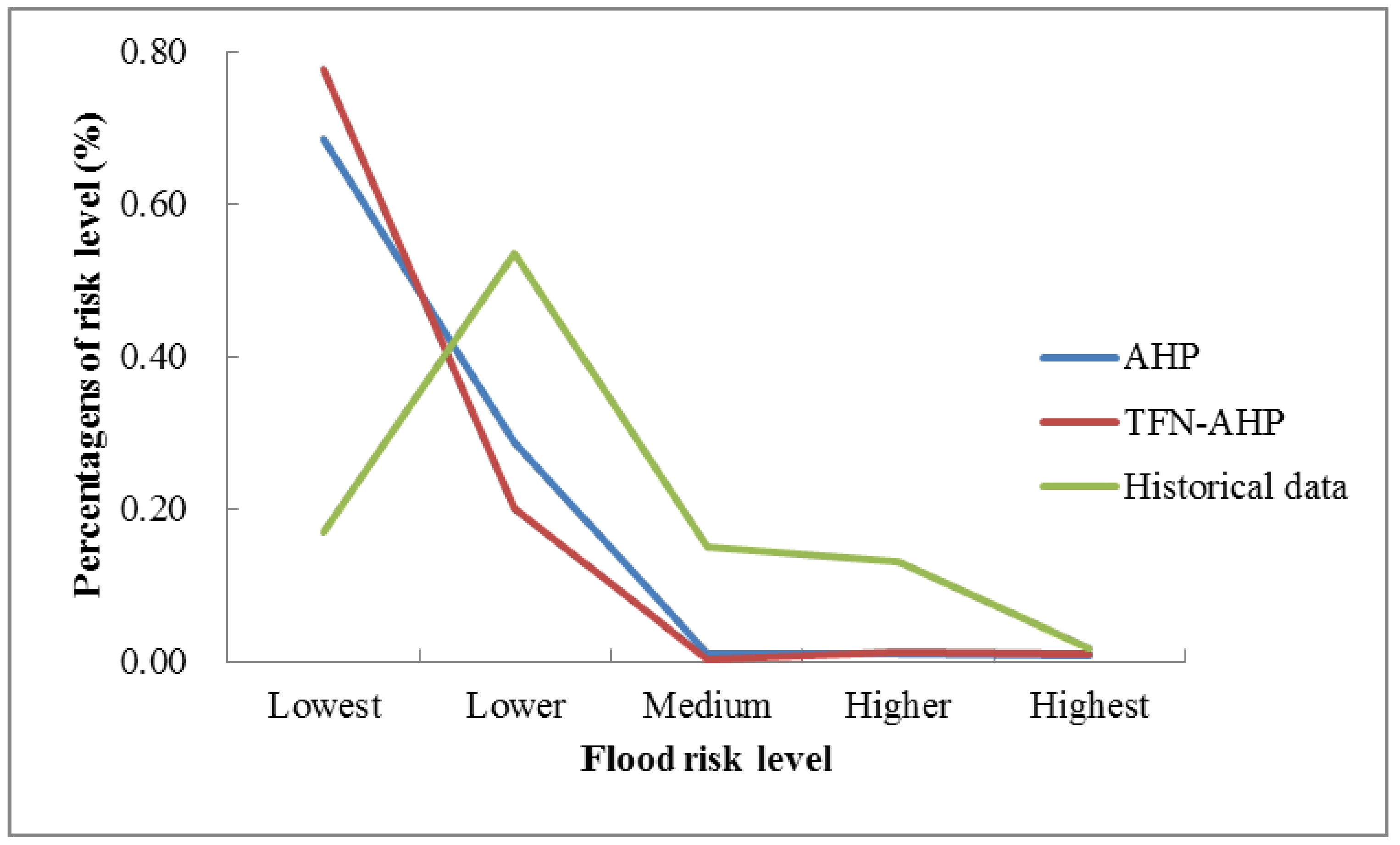
  • The comparison between AHP and TFN-AHP demonstrated that TFN-AHP is more effective with relatively higher accuracy, particularly in the hazard and exposure layers. The flood-risk maps were consistent with flooding risk regions obtained from historical data, especially for the high-risk regions.
  • The results of Global Moran’s I index showed that there exists a spatial autocorrelation of flood risk in Chongqing. Further, the indication of Anselin Local Moran’s I was the spatial distribution of hot spots, mainly located in main urban areas and areas along the Yangtze River all year round in Chongqing.
  • The results of the sensitivity analysis revealed three groups with various sensitivity to weight changes. Indicators like V4 are the most sensitive, followed by factors such as E2, E3 and E4, and indexes like H1.
Overall, it can be seen that some specific environmental characteristics of mountain cities were fully considered through TFN-AHP. The experimental consequences indicate that the proposed method can be employed in early prediction for mountain cities with higher accuracy. Nonetheless, further investigations should be conducted to have implications for highly accurate evaluation. For instance, TFN-AHP should be combined with other approaches in the future, such as the entropy weight method, to alleviate subjectivity. Additionally, the data of assessment factors should be extended to make evaluation outcomes more consistent with the actual situations.

Author Contributions

S.C.: Conceptualization, Supervision, Validation, Methodology, Writing—review and editing; J.F.: Formal analysis, Investigation, Validation, Visualization, Writing—original draft; W.Y.: Conceptualization, Supervision, Validation, Methodology, Writing—review and editing. All authors have read and agreed to the published version of the manuscript.

Funding

This research was funded by the Fundamental Research Funds for the Central Universities (Project No. 2018CDJSK03XK01), Philosophy and social science planning research project of Chongqing Social Science Planning Office (Grants #2020YBGL88) and the Chongqing Technology Innovation and Application Development Key Project (No. ctsc2019jscx-gksbX0066).

Institutional Review Board Statement

Not applicable.

Informed Consent Statement

Not applicable.

Data Availability Statement

The data and the website of data sources used to support the findings of this study are included within the article. The detailed data used to support the findings of this study are available from the corresponding author upon request.

Conflicts of Interest

The authors declare no conflict of interest.

References

  1. Sun, R.; Gong, Z.; Gao, G.; Shah, A.A. Comparative analysis of Multi-Criteria Decision-Making methods for flood disaster risk in the Yangtze River Delta. Int. J. Disaster Risk Reduct. 2020, 51, 101768. [Google Scholar] [CrossRef]
  2. Lyu, H.-M.; Shen, S.-L.; Zhou, A.; Yang, J. Perspectives for flood risk assessment and management for mega-city metro system. Tunn. Undergr. Space Technol. 2019, 84, 31–44. [Google Scholar] [CrossRef]
  3. Petit-Boix, A.; Sevigne-Itoiz, E.; Rojas-Gutierrez, L.A.; Barbassa, A.P.; Josa, A.; Rieradevall, J.; Gabarrell, X. Floods and consequential life cycle assessment: Integrating flood damage into the environmental assessment of stormwater Best Management Practices. J. Clean. Prod. 2017, 162, 601–608. [Google Scholar] [CrossRef] [Green Version]
  4. Cai, T.; Li, X.Y.; Ding, X.; Wang, J.; Zhan, J. Flood risk assessment based on hydrodynamic model and fuzzy comprehensive evaluation with GIS technique. Int. J. Disaster Risk Reduct. 2019, 35, 101077. [Google Scholar] [CrossRef]
  5. Sarmah, T.; Das, S.; Narendr, A.; Aithal, B.H. Assessing human vulnerability to urban flood hazard using the analytic hierarchy process and geographic information system. Int. J. Disaster Risk Reduct. 2020, 50, 101659. [Google Scholar] [CrossRef]
  6. Fang, J.; Hu, J.; Shi, X.; Zhao, L. Assessing disaster impacts and response using social media data in China: A case study of 2016 Wuhan rainstorm. Int. J. Disaster Risk Reduct. 2019, 34, 275–282. [Google Scholar] [CrossRef]
  7. Sajjad, M.; Chan, J.C.L.; Kanwal, S. Integrating spatial statistics tools for coastal risk management: A case-study of typhoon risk in mainland China. Ocean Coast. Manag. 2020, 184, 105018. [Google Scholar] [CrossRef]
  8. Thaler, T.; Hartmann, T. Justice and flood risk management: Reflecting on different approaches to distribute and allocate flood risk management in Europe. Nat. Hazards 2016, 83, 129–147. [Google Scholar] [CrossRef] [Green Version]
  9. Romanescu, G.; Hapciuc, O.E.; Minea, I.; Iosub, M. Flood vulnerability assessment in the mountain-plateau transition zone: A case study of Marginea village (Romania). J. Flood Risk Manag. 2018, 11, S502–S513. [Google Scholar] [CrossRef]
  10. Sakamoto, T.; Van Nguyen, N.; Kotera, A.; Ohno, H.; Ishitsuka, N.; Yokozawa, M. Detecting temporal changes in the extent of annual flooding within the Cambodia and the Vietnamese Mekong Delta from MODIS time-series imagery. Remote Sens. Environ. 2007, 109, 295–313. [Google Scholar] [CrossRef]
  11. Williams, P.; Kliskey, A.; McCarthy, M.; Lammers, R.; Alessa, L.; Abatzoglou, J. Using the Arctic water resources vulnerability index in assessing and responding to environmental change in Alaskan communities. Clim. Risk Manag. 2019, 23, 19–31. [Google Scholar] [CrossRef]
  12. Fan, Q.; Tian, Z.; Wang, W. Study on Risk Assessment and Early Warning of Flood-Affected Areas when a Dam Break Occurs in a Mountain River. Water 2018, 10, 1369. [Google Scholar] [CrossRef] [Green Version]
  13. Lin, K.; Chen, H.; Xu, C.-Y.; Yan, P.; Lan, T.; Liu, Z.; Dong, C. Assessment of flash flood risk based on improved analytic hierarchy process method and integrated maximum likelihood clustering algorithm. J. Hydrol. 2020, 584, 124696. [Google Scholar] [CrossRef]
  14. Zhang, J.Y.; Chen, Y.B. Risk Assessment of Flood Disaster Induced by Typhoon Rainstorms in Guangdong Province, China. Sustainability 2019, 11, 2738. [Google Scholar] [CrossRef] [Green Version]
  15. Terzi, S.; Torresan, S.; Schneiderbauer, S.; Critto, A.; Zebisch, M.; Marcomini, A. Multi-risk assessment in mountain regions: A review of modelling approaches for climate change adaptation. J. Environ. Manag. 2019, 232, 759–771. [Google Scholar] [CrossRef] [PubMed]
  16. Qianzhu, Z.; Huoming, Z.; Yang, L.; Ruiyi, Z.; Qiang, G.; Jianmei, Y.; Kun, S. Research on Chongqing Mountain Flood Disaster Risk Assessment System Based on AHP-GIS. In IOP Conference Series: Earth and Environmental Science; IOP Publishing: Bristol, UK, 2019; Volume 330. [Google Scholar] [CrossRef]
  17. Black, A.R.; Burns, J.C. Re-assessing the flood risk in Scotland. Sci. Total. Environ. 2002, 294, 169–184. [Google Scholar] [CrossRef]
  18. Newman, J.P.; Maier, H.R.; Riddell, G.A.; Zecchin, A.C.; Daniell, J.E.; Schaefer, A.M.; van Delden, H.; Khazai, B.; O’Flaherty, M.J.; Newland, C.P. Review of literature on decision support systems for natural hazard risk reduction: Current status and future research directions. Environ. Model. Softw. 2017, 96, 378–409. [Google Scholar] [CrossRef]
  19. Gigovic, L.; Pamucar, D.; Bajic, Z.; Drobnjak, S. Application of GIS-Interval Rough AHP Methodology for Flood Hazard Mapping in Urban Areas. Water 2017, 9, 360. [Google Scholar] [CrossRef] [Green Version]
  20. Lyu, H.-M.; Shen, S.-L.; Zhou, A.-N.; Zhou, W.-H. Flood risk assessment of metro systems in a subsiding environment using the interval FAHP-FCA approach. Sustain. Cities Soc. 2019, 50, 101682. [Google Scholar] [CrossRef]
  21. Wang, X.W.; Xie, H.J. A Review on Applications of Remote Sensing and Geographic Information Systems (GIS) in Water Resources and Flood Risk Management. Water 2018, 10, 608. [Google Scholar] [CrossRef] [Green Version]
  22. Yin, Z.e.; Yin, J.; Xu, S.; Wen, J. Community-based scenario modelling and disaster risk assessment of urban rainstorm waterlogging. J. Geogr. Sci. 2011, 21, 274–284. [Google Scholar] [CrossRef]
  23. Lin, T.; Liu, X.F.; Song, J.C.; Zhang, G.Q.; Jia, Y.Q.; Tu, Z.Z.; Zheng, Z.H.; Liu, C.L. Urban waterlogging risk assessment based on internet open data: A case study in China. Habitat Int. 2018, 71, 88–96. [Google Scholar] [CrossRef]
  24. Lyu, H.-M.; Zhou, W.-H.; Shen, S.-L.; Zhou, A.-N. Inundation risk assessment of metro system using AHP and TFN-AHP in Shenzhen. Sustain. Cities Soc. 2020, 56, 102103. [Google Scholar] [CrossRef]
  25. Yang, X.L.; Ding, J.H.; Hou, H. Application of a triangular fuzzy AHP approach for flood risk evaluation and response measures analysis. Nat. Hazards 2013, 68, 657–674. [Google Scholar] [CrossRef]
  26. Enaruvbe, G.; Yesuf, G. Spatial analysis of flood disaster in Delta State, Nigeria. Ife Res. Publ. Geogr. 2016, 11, 52–58. [Google Scholar]
  27. Zhao, M.; Sun, Z.; Zeng, Y. Exploring urban risk reduction strategy based on spatial statistics and scenario planning. J. Clean. Prod. 2020, 264, 121688. [Google Scholar] [CrossRef]
  28. Santos, M.; Bateira, C.; Soares, L.; Hermenegildo, C. Hydro-geomorphologic GIS database in Northern Portugal, between 1865 and 2010: Temporal and spatial analysis. Int. J. Disaster Risk Reduct. 2014, 10, 143–152. [Google Scholar] [CrossRef]
  29. Guo, N.J.; Ren, Y.J.; Tang, X.L. The temporal and spatial evolution of natural disasters in China. Geojournal 2019, 84, 1515–1530. [Google Scholar] [CrossRef]
  30. Huang, C.; Chen, Y.; Wu, J. Mapping spatio-temporal flood inundation dynamics at large river basin scale using time-series flow data and MODIS imagery. Int. J. Appl. Earth Obs. Geoinf. 2014, 26, 350–362. [Google Scholar] [CrossRef]
  31. Bathrellos, G.D.; Skilodimou, H.D.; Soukis, K.; Koskeridou, E. Temporal and spatial analysis of flood occurrences in the drainage basin of pinios river (thessaly, central greece). Land 2018, 7, 106. [Google Scholar] [CrossRef] [Green Version]
  32. Ovando, A.; Martinez, J.-M.; Tomasella, J.; Rodriguez, D.A.; von Randow, C. Multi-temporal flood mapping and satellite altimetry used to evaluate the flood dynamics of the Bolivian Amazon wetlands. Int. J. Appl. Earth Obs. Geoinf. 2018, 69, 27–40. [Google Scholar] [CrossRef]
  33. Zhao, J.; Jin, J.; Xu, J.; Guo, Q.; Hang, Q.; Chen, Y. Risk assessment of flood disaster and forewarning model at different spatial-temporal scales. Theor. Appl. Clim. 2018, 132, 791–808. [Google Scholar] [CrossRef]
  34. Fang, D.X.; Dong, X.N.; Deng, C.; Wu, Z.; Hai, C.; Gao, S.; Huang, A.N. The temporal and spatial distribution characteristics of precipitation in Chongqing from 2008 to 2016. Atmos. Sci. 2020, 44, 327–340. (In Chinese) [Google Scholar]
  35. Zhong, C.; Ren, X.M.; Zhou, X.Q.; Luo, L.X.; Wang, J.L.; Li, Y.N. The temporal and spatial distribution of precipitation in Chongqing. J. Sichuan Norm. Univ. Nat. Sci. Ed. 2003, 171–176. (In Chinese) [Google Scholar] [CrossRef]
  36. News, C. Protecting the Three Gorges Reservoir Is Still the Core Task of Chongqing Water Conservancy during the “14th Five-Year Plan” Period. 2020. Available online: https://baijiahao.baidu.com/s?id=1683873717686562323&wfr=spider&for=pc (accessed on 17 April 2021).
  37. Lyu, H.-M.; Shen, S.-L.; Zhou, A.; Zhou, W.-H. Data in flood risk assessment of metro systems in a subsiding environment using the interval FAHP-FCA approach. Data Brief 2019, 26, 104468. [Google Scholar] [CrossRef] [PubMed]
  38. Rahmati, O.; Zeinivand, H.; Besharat, M. Flood hazard zoning in Yasooj region, Iran, using GIS and multi-criteria decision analysis. Geomatics Nat. Hazards Risk 2016, 7, 1000–1017. [Google Scholar] [CrossRef] [Green Version]
  39. Zhang, N.; Alipour, A. Multi-scale robustness model for highway networks under flood events. Transport. Res. Part D Transport. Environ. 2020, 83, 102281. [Google Scholar] [CrossRef]
  40. Sugumaran, R.; Larson, S.R.; DeGroote, J.P. Spatio-temporal cluster analysis of county-based human West Nile virus incidence in the continental United States. Int. J. Health Geogr. 2009, 8, 1–19. [Google Scholar] [CrossRef] [Green Version]
  41. Ghosh, K.G. Analysis of Rainfall Trends and its Spatial Patterns During the Last Century over the Gangetic West Bengal, Eastern India. J. Geovisualization Spat. Anal. 2018, 2, 15. [Google Scholar] [CrossRef]
  42. Berta, A.A.; Eyasu, E.; Teshome, S.; Legese, F.G. Land use/land cover change effect on soil erosion and sediment delivery in the Winike watershed, Omo Gibe Basin, Ethiopia. Sci. Total Environ. 2020, 728, 138776. [Google Scholar] [CrossRef]
  43. Yuping, C.; Hui, Y.; Yijuan, Y.; Chunling, Z.; Ping, G.; Liyue, Z.; Liya, F.; Daiqi, Y. Relationships of ozone formation sensitivity with precursors emissions, meteorology and land use types, in Guangdong-Hong Kong-Macao Greater Bay Area, China. J. Environ. Sci. 2020, 94, 1–13. [Google Scholar] [CrossRef]
  44. Xiao, Y.; Yi, S.; Tang, Z. Integrated flood hazard assessment based on spatial ordered weighted averaging method considering spatial heterogeneity of risk preference. Sci. Total Environ. 2017, 599, 1034–1046. [Google Scholar] [CrossRef]
  45. Yariyan, P.; Avand, M.; Abbaspour, R.A.; Torabi Haghighi, A.; Costache, R.; Ghorbanzadeh, O.; Janizadeh, S.; Blaschke, T. Flood susceptibility mapping using an improved analytic network process with statistical models. Nat. Hazards Risk 2020, 11, 2282–2314. [Google Scholar] [CrossRef]
  46. Surwase, T.; Manjusree, P.; Nagamani, P.V.; Jaisankar, G. Novel technique for developing flood hazard map by using AHP: A study on part of Mahanadi River in Odisha. SN Appl. Sci. 2019, 1, 1196. [Google Scholar] [CrossRef] [Green Version]
  47. Ali, S.A.; Parvin, F.; Pham, Q.B. GIS-based comparative assessment of flood susceptibility mapping using hybrid multi-criteria decision-making approach, naïve Bayes tree, bivariate statistics and logistic regression: A case of Topľa basin, Slovakia. Ecol. Indic. 2020, 117, 106620. [Google Scholar] [CrossRef]
  48. McMahan, B.; Gerlak, A.K. Climate risk assessment and cascading impacts: Risks and opportunities for an electrical utility in the U.S. Southwest. Clim. Risk Manag. 2020, 29, 100240. [Google Scholar] [CrossRef]
  49. Lawrence, J.; Blackett, P.; Cradock-Henry, N.A. Cascading climate change impacts and implications. Clim. Risk Manag. 2020, 29, 100234. [Google Scholar] [CrossRef]
Figure 1. Location of the study area: (a) China, (b) Chongqing.
Atmosphere 12 00623 g001
Figure 2. Flowchart of the flood risk assessment for Chongqing. Note: DR means the daily rainfall of counties and GDP is Gross Domestic Product of each county in Chongqing.
Atmosphere 12 00623 g002
Figure 3. Triangular membership function.
Atmosphere 12 00623 g003
Figure 4. Triangular fuzzy affiliation of indicators.
Atmosphere 12 00623 g004
Figure 5. Spatial distribution map of flood hazard in four seasons during 2018: (a) Spring—AHP, (b) Spring—TFN-AHP, (c) Summer—AHP, (d) Summer—TFN-AHP, (e) Fall—AHP, (f) Fall—TFN-AHP, (g) Winter—AHP, (h) Winter—TFN-AHP.
Atmosphere 12 00623 g005aAtmosphere 12 00623 g005b
Figure 6. Spatial distribution map of flood exposure: (a) AHP, (b) TFN-AHP.
Atmosphere 12 00623 g006
Figure 7. Spatial distribution map of normalized exposure data: (a) elevation, (b) slope, (c) river network proximity, (d) river network density.
Atmosphere 12 00623 g007
Figure 8. Spatial distribution map of normalized vulnerability data: (a) population density, (b) average GDP, (c) per capita disposable income, (d) road network density, (e) land use type.
Atmosphere 12 00623 g008
Figure 9. Spatial distribution map of flood vulnerability: (a) AHP, (b) TFN-AHP.
Atmosphere 12 00623 g009
Figure 10. Spatial distribution of the flood risk in four seasons of Chongqing: (a) flood risk in spring—AHP, (b) flood risk in spring—TFN-AHP, (c) flood risk in summer—AHP, (d) flood risk in summer—TFN-AHP, (e) flood risk in fall—AHP, (f) flood risk in fall—TFN-AHP, (g) flood risk in winter—AHP, (h) flood risk in winter—TFN-AHP.
Atmosphere 12 00623 g010aAtmosphere 12 00623 g010b
Figure 11. Distribution map of local spatial autocorrelation: (a) Spring, (b) Summer, (c) Fall, (d) Winter. Note: Not significant means that the representative flood risk has no significant spatial relationship in this area. High-high cluster and low-low cluster are the identification of high- and low-risk spots. High-low outlier and low-high outlier are used to convey that the hot spots and the cold spots are mixed with each other, which makes it impossible to identify the specific flood risk value in this region.
Atmosphere 12 00623 g011aAtmosphere 12 00623 g011b
Figure 12. Sensitivity analysis results: (a) H1, (b) E2, (c) E3, (d) E4, (e) V4. R1 = Very low risk, R2 = Low risk, R3 = Moderate risk, R4 = High risk, R5 = Very high risk.
Atmosphere 12 00623 g012aAtmosphere 12 00623 g012b
Figure 13. Percentages of flood risk of all levels.
Atmosphere 12 00623 g013
Table 1. Data sources.
Data NameData TypeSource
Climate dataAverage annual precipitation in countiesChina Meteorological Data Network (http://data.cma.cn/, accessed on 11 May 2021)
Rainstorm frequency, annual precipitation
Terrain dataThe Digital Elevation Model (DEM)Geospatial Data Cloud (http://www.gscloud.cn/, accessed on 11 May 2021)
Socio-economic dataPopulation density, average area GDPthe Global Change Scientific Research Data Publishing System (http://www.geodoi.ac.cn/WebCn/Default.aspx, accessed on 11 May 2021)
Per capita disposable incomeChongqing Statistical Yearbook (http://data.tjj.cq.gov.cn/, accessed on 11 May 2021)
Land cover typesthe National Geographic Information Directory Service System (http://www.webmap.cn/main.do?method=index accessed on 17 April 2021)
Road and river networkOpenStreetMap (https://www.openstreetmap.org/ accessed on 17 April 2021)
Table 2. Quantitative scale of triangular fuzzy number in TFN-AHP.
Linguistic TermsFuzzy NumberTriangular Fuzzy ScaleReciprocal Triangular Fuzzy Number
Equally important1(1, 1, 1)(1, 1, 1)
Almost equally important1′(1, 1, 3)(1/3, 1, 1)
Intermediate value2′(1, 2, 4)(1/4, 1/2, 1)
Moderately more important3′(1, 3, 5)(1/5, 1/3, 1)
Intermediate value4′(2, 4, 6)(1/6, 1/4, 1/2)
Strongly more important5′(3, 5, 7)(1/7, 1/5, 1/3)
Intermediate value6′(4, 6, 8)(1/8, 1/6, 1/4)
Very strongly more important7′(5, 7, 9)(1/9, 1/7, 1/5)
Intermediate value8′(6, 8, 10)(1/10, 1/8, 1/6)
Extremely more important9′(7, 9, 11)(1/11, 1/9, 1/7)
Table 3. AHP and TFN-AHP process weight.
IndexLayerAHP (W0)PiTFN-AHP (W0) AHP (Wb)PiTFN-AHP (Wb)
H0.540(0.132, 0.25, 0.732)0.454H10.667(0.250, 0.750, 1.875)0.574
H20.333(0.150, 0.250, 0.625)0.426
E0.163(0.093, 0.25, 0.439)0.233E10.278(0.113, 0.327, 1.042)0.318
E20.160(0.122, 0.420, 1.042)0.157
E30.095(0.069, 0.132, 0.481)0.194
E40.467(0.048, 0.121, 0.280)0.332
V0.297(0.176, 0.5, 1.318)0.313V10.354(0.073, 0.249, 0.764)0.3
V20.269(0.092, 0.283, 0.764)0.291
V30.188(0.094, 0.240, 0.623)0.27
V40.112(0.082, 0.179, 0.462)0.076
V50.078(0.025, 0.048, 0.124)0.063
Table 4. Index layer weights determined by TFN-AHP.
Index LayerHEVPi
H(1, 1, 1)(1, 1, 3)(0.25, 0.5, 1)(0.033, 0.057, 0.201)
E(0.33, 1, 1)(1, 1, 1)(0.25, 0.5, 1)(0.023, 0.057, 0.121)
V(1, 2, 4)(1, 2, 4)(1, 1, 1)(0.044, 0.113, 0.362)
Table 5. Hazard layer weights determined by TFN-AHP.
Sub-Index LayerH1H2Pi
H1(1, 1, 1)(1, 3, 5)(0.250, 0.750, 1.875)
H2(0.2, 0.33, 1)(1, 1, 1)(0.150, 0.250, 0.625)
Table 6. Exposure layer weights determined by TFN-AHP.
Sub-Index LayerE1E2E3E4Pi
E1(1, 1, 1)(1, 1, 3)(1, 2, 4)(1, 3, 5)(0.113, 0.327, 1.042)
E2(0.33, 1, 1)(1, 1, 1)(1, 3, 5)(2, 4, 6)(0.122, 0.420, 1.042)
E3(0.25, 0.5, 1)(0.2, 0.33, 1)(1, 1, 1)(1, 1, 3)(0.069, 0.132, 0.481)
E4(0.2, 0.33, 1)(0.17, 0.25, 0.5)(0.33, 1, 1)(1, 1, 1)(0.048, 0.121, 0.280)
Table 7. Vulnerability layer weights determined by TFN-AHP.
Sub-Index LayerV1V2V3V4V5Pi
V1(1, 1, 1)(1, 2, 4)(1, 3, 5)(1, 3, 5)(1, 2, 4)(0.073, 0.249, 0.764)
V2(0.25, 0.5, 1)(1, 1, 1)(2, 4, 6)(1, 3, 5)(2, 4, 6)(0.092, 0.283, 0.764)
V3(0.2, 0.33, 1)(0.17, 0.25, 0.5)(1, 1, 1)(2, 4, 6)(3, 5, 7)(0.094, 0.240, 0.623)
V4(0.2, 0.33, 1)(0.2, 0.33, 1)(0.17, 0.25, 0.5)(1, 1, 1)(4, 6, 8)(0.082, 0.179, 0.462)
V5(0.25, 0.5, 1)(0.17, 0.25, 0.5)(0.14, 0.2, 0.33)(0.125, 0.17, 0.25)(1, 1, 1)(0.025, 0.048, 0.124)
Table 8. Global Moran’s I analysis on the risk level of heavy rain and flood in Chongqing.
VariableSpringSummerFallWinter
Z38.2854.3434.6949.62
P0000
Table 9. The definitions of flood risk.
Level Flood Risk Value
Very low risk <0.1
Low risk 0.1–0.3
Moderate risk 0.3–0.7
High risk 0.7–0.9
Very high risk >0.9
The flood risk values are standardized in GIS before classification.
Publisher’s Note: MDPI stays neutral with regard to jurisdictional claims in published maps and institutional affiliations.

