Article

The Role of the Atmospheric Aerosol in Weather Forecasts for the Iberian Peninsula: Investigating the Direct Effects Using the WRF-Chem Model

1
Department of Environment and Planning & CESAM, University of Aveiro, 3810-193 Aveiro, Portugal
2
Institute of Electronics and Informatics Engineering of Aveiro (IEETA), University of Aveiro, 3810-193 Aveiro, Portugal
3
Center for R&D in Mathematics and Applications (CIDMA), University of Aveiro, 3810-193 Aveiro, Portugal
4
CEMAT and Department of Mathematics, Instituto Superior Técnico, University of Lisbon, 1049-001 Lisbon, Portugal
*
Author to whom correspondence should be addressed.
Atmosphere 2021, 12(2), 288; https://doi.org/10.3390/atmos12020288
Submission received: 13 January 2021 / Revised: 18 February 2021 / Accepted: 19 February 2021 / Published: 23 February 2021
(This article belongs to the Special Issue Climate Change and Air Pollution in Portugal)

Abstract

:
In the atmosphere, aerosols play an important role in climate change, the Earth’s environment and human health. The purpose of this study is to investigate the direct and semi-direct aerosol effects on weather forecasting, focusing on the Iberian Peninsula (IP). To that end, two Weather Research and Forecasting (WRF)-Chem simulations (with and without aerosol feedback) for an entire year (2015) were performed. The model setup includes two nested domains run in two-way mode, allowing the downscaling for the IP domain at a 5 × 5 km2 high-horizontal resolution. The results were explored through agreement of pairs of time series and their spatial variability in order to analyse the importance of including the online-coupled aerosol radiative effect on the meteorological variables: shortwave (solar) radiation, air temperature and precipitation. Significant variations of agreement were found when capturing both temporal and spatial patterns of the analysed meteorological variables. While the spatial distribution of temperature and precipitation is similar throughout the IP domain, with agreement values ranging from 0.87 up to 1.00, the solar radiation presents a distinct spatial pattern with lower agreement values (0.68–0.75) over ocean and higher agreement (0.75–0.98) over land regions. With regard to the spatial differences between simulations, the aerosol contributed to a considerable decrease in annual mean and maximum radiation (up to 20 and 40 Wm−2, respectively), slightly impacting the temperature variation (up to 0.5 °C). These results suggest that the aerosol feedback effects should be accounted when performing weather forecasts, and not only for purposes of air quality assessment.

1. Introduction

The production of realistic and operational weather forecasts is essential for understanding atmospheric dynamics and resulting phenomena, such as heatwaves and heavy rain [1,2,3]. For this purpose, taking advantage of the rapid increase in computational power, the weather prediction community has been working to increase the complexity of the numerical models, using higher resolutions to explicitly resolve fronts, convective systems, local wind systems and clouds [2]. In extreme weather conditions, these numerical weather predictions (NWP) have a vital role in preparing emergency responses in order to prevent disasters [2,4,5]. In addition, NWP are also used for offline regional/urban air quality applications, where the meteorological simulation outputs are used as inputs for a chemical transport model (CTM). These offline approaches discard, on one hand, the influence that the atmospheric composition might have on both weather and climate and, on the other hand, can lead to a loss of important information about physical and chemical processes occurring on a time scale much smaller than the frequency of the meteorological model outputs [2,6,7]. Nevertheless, most meteorology-chemistry modelling systems remain to be driven in offline mode [1,8], since the offline coupling has a low computational cost, especially if the meteorological outputs are already available. Hence they are of particular interest to test different physical and chemical assumptions (e.g., land use, emissions) and there is more flexibility in ensemble modelling exercises [2,9].
To overcome the methodological weaknesses related with offline applications, throughout the last three decades a new generation of online coupled meteorology and chemistry models has been developed and improved in order to represent the complex aerosol–cloud radiation feedbacks [2,10]. Baklanov et al. [1] distinguish two ways of online coupling: (i) online integrated models sharing the same grids and time step to simulate meteorology and chemistry; and (ii) online access models using independent meteorology and chemistry modules that can be run on different simulation grids, but with a regular and frequent exchange of meteorology and chemistry data. Besides these two-way interactions, online models are more consistent in describing physical and chemical processes, mainly in higher resolutions, since no time and space interpolations are required and the same parametrizations for computing meteorology and chemistry are used [2,6,11]. Thereby, the application of online models instead of the traditional offline modelling systems is becoming increasingly popular, in particular for air quality modelling purposes from regional to urban scales, although they are more computationally demanding [1,12].
From the point of view of the weather predictions, the expected total impact of atmospheric aerosol particles can be divided into direct, semi-direct and indirect effects. The magnitude and sign of these effects are dependent on optical, physical and chemical aerosol properties, microphysics schemes and spatial (over land or sea) and vertical distributions of the aerosol layer and cloud cover, thus modifying the Earth’s radiative budget, as well as the microphysics through the clouds formation (only semi-direct and indirect effects) [13,14,15].
Direct effects involve the scattering of solar radiation and subsequent reduction in the amount of shortwave radiation reaching the Earth’s surface, whereas the semi-direct effects are associated with the absorption of solar radiation by black carbon and other absorbing aerosol compounds, producing a change in the ground surface temperature, relative humidity and atmospheric stability impacting the clouds formation. By definition, the computation of shortwave radiation requires information on both incoming solar radiation and solar declination (i.e., Sun’s position), taking into account the absorption, reflection and scattering of solar radiation that occurs into the atmosphere and on the Earth’s surface at different times of the year and day. In turn, indirect effects reflect the role of the aerosol particles acting as cloud condensation nuclei and/or ice nuclei, thus influencing the cloud microphysical, radiative and thermodynamic properties (“first indirect effect”) and, consequently, the cloud cover, lifetime of clouds and precipitation can also be affected (“second indirect effect”) [7,15,16,17,18,19,20]. In addition, aerosol–cloud interactions under atmospheric cooling can also contribute to an additional latent heat release due to freezing of greater amount of cloud water. As a result, this thermodynamic invigoration effect of aerosols often leads to an increase in cloud cover, cloud-top height and cloud thickness [21,22]. In order to evaluate the aerosol–meteorology feedback effects, several studies involving online models have been performed over different Earth regions and in distinct aerosol concentration gradients. An ensemble exercise with eight online models applied for the year 2010 over simulation domains covering the Europe, North America or both, showed larger differences between models than differences between simulations with and without aerosol feedback using the same model. This conclusion demonstrates that the aerosol effect on NWP may depend significantly on the chosen online modelling system and used configurations [12,23]. When aerosol optical properties were incorporated into the radiation schemes, ref. [14] obtained shortwave radiation values were closer to the observations; however, these were still underestimated. In contrast, when aerosol effects were neglected, the predicted solar radiation was much higher than the observations. This poor modelling performance is more evident over regions with higher aerosol loadings [2,24,25]. To test the sensitivity of aerosol–meteorology feedbacks over regions with high aerosol concentrations, several studies over East Asia [4,18,26,27], as well as studies to reproduce Russian forest fires and Saharan dust episodes [12,28], were performed using the online Weather Research and Forecasting (WRF)-Chem model. Overall, reductions in the surface net radiation, 2 m temperature, 10 m wind speed, atmospheric boundary layer (ABL) height and precipitation were estimated. These reductions, in turn, led to changes in the chemical predictions by decreasing the atmospheric dispersion, wet scavenging and photolysis rate of air pollutants. In East Asia, comparing the magnitude of the aerosol effects with similar tests for Europe and the U.S.A., larger and more robust effects are expected, which can be explained by the higher aerosol concentrations and cloud cover [19,26]. Nevertheless, the total aerosol effect is underestimated, largely contributing to this result the approach used in WRF-Chem for estimating the indirect aerosol effects [28,29,30,31,32,33]. For the forest fire and dust cases, the best model performance was obtained from simulations including only direct aerosol effects. When indirect aerosol effects were quantified, more pronounced and persistent aerosol–cloud radiation feedback was felt over ocean regions, although with large uncertainties in the clouds’ representation (type, lifetime, location, extent). Therefore, further research to improve and develop new cloud microphysics parametrization is required [7,11,13,28,32]. This is particularly essential in certain geographic regions, such as the Iberian Peninsula, where different types of natural and anthropogenic sources of aerosols co-exist on daily basis [34], together with specific and complex meteorological patterns, which result in high levels of aerosol concentrations [35].
Based on these scientific developments about atmospheric aerosol–meteorology feedback, and especially over the Iberian Peninsula region, the most accurate modelling approaches and a few less explored aspects are highlighted in this paper: (i) testing direct and semi-direct aerosol effects on the weather; (ii) simulating a full year with high resolutions; and (iii) evaluating the seasonal cycle of aerosol effects on meteorological variables through agreement metrics. Thereby, this study aims to investigate the influence of the direct and semi-direct aerosol effects on meteorological variables (shortwave radiation, air temperature and precipitation) using the online WRF-Chem model. To that end, two WRF-Chem simulations (with and without aerosol feedback) under two nested domains were performed for the year 2015, focusing the analysis on the inner domain (Iberian Peninsula).

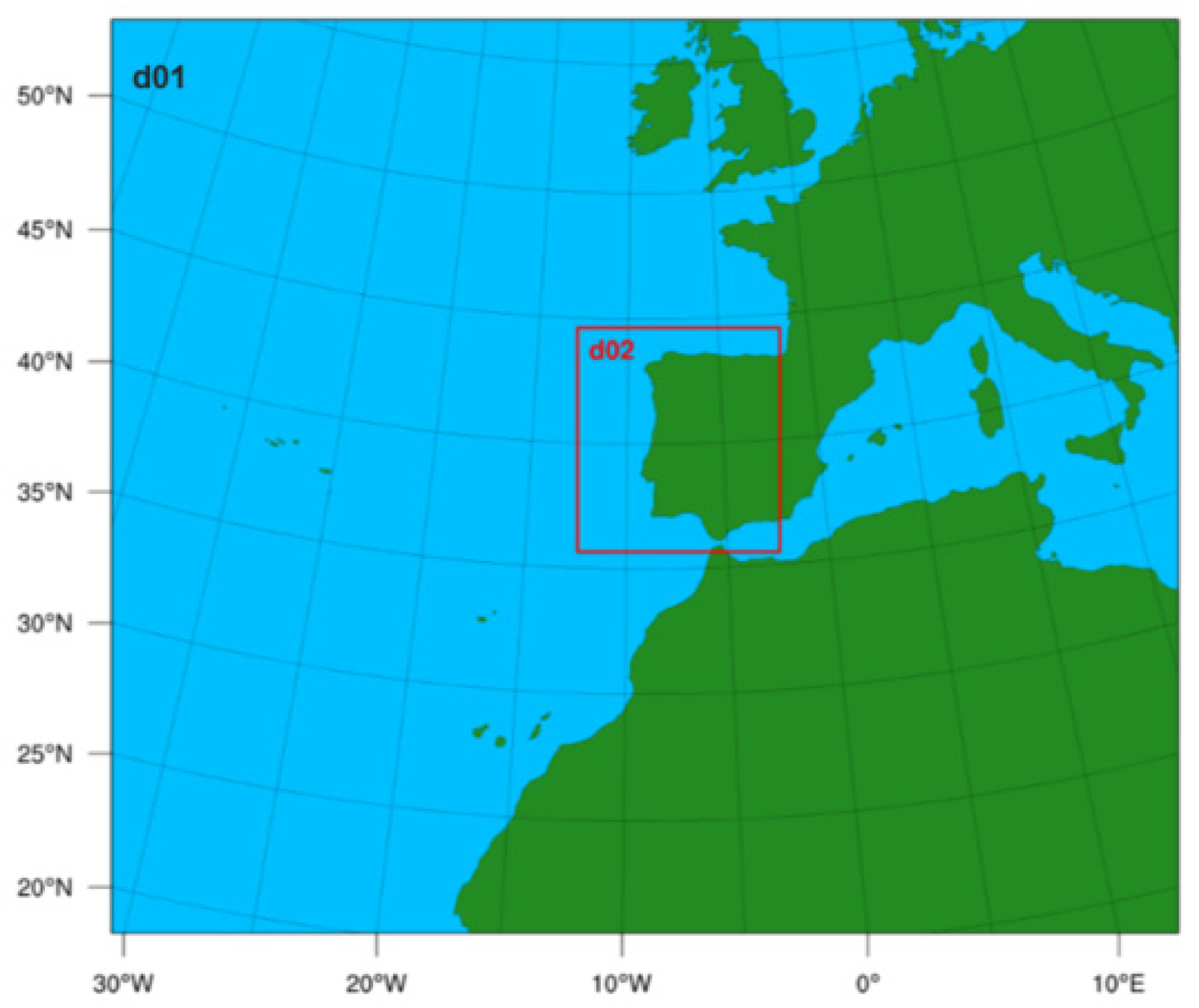
2. Model Configurations and Input Data

With the purpose of assessing the direct and semi-direct effects of the atmospheric aerosol on the targeted meteorological variables, the WRF-Chem version 3.6.1 was used. The WRF-Chem is an online model with fully coupled chemistry within the Weather Research and Forecasting (WRF) model that allows us to simultaneously predict the meteorological and chemical components. Hence, the same simulation grids (i.e., horizontal and vertical levels), physical parametrizations, transport schemes, vertical mixing and timestep are shared, enabling aerosol–meteorology feedback [14,36]. To test the sensitivity of the aerosol effect on the meteorology, two WRF-Chem simulations, with and without aerosol feedback including direct and semi-direct effects and aerosol optical properties, were carried out on a daily basis with hourly resolution for the one-year period: from 24 December 2014 to 31 December 2015. The days of December 2014 were discarded as model spin-ups. The decision to simulate the year 2015 was supported by a weather data series provided from public institutions and information reported from the World Meteorological Organization (WMO), which indicated that 2015 was one of the hottest and driest years in Europe within a recent 30-year period (1981–2010), with more frequent and prolonged extreme events (e.g., heatwaves, droughts) [37]. Regarding the atmospheric aerosol levels, annual and daily limit values (LV) set by the Directive 2008/50/EC of the European Parliament and of the Council of 21 May 2008 on ambient air quality and cleaner air for Europe were not exceeded in 2015 for most European monitoring sites, mainly in southwestern Europe (75th percentiles of the daily LV for both PM10 and PM2.5 were around 40 and 12 µg.m−3). However, some exceedances were measured, which are related with PM10 pollution episodes that occurred in February, March and October due to a complex combination of different anthropogenic and natural sources, with higher preponderance attributed to emissions from residential combustion, agriculture and Saharan dust intrusions [38].
The simulations were conducted over two nested domains in two-way mode, starting with a coarse domain covering a large part of Europe and North Africa (d01, 25 km horizontal resolution), and then a regional domain focused on the Iberian Peninsula (IP) (d02, 5 km horizontal resolution) (Figure 1). The vertical structure of the atmosphere was resolved with 29 vertical levels extending up to 50 hPa, with the lowest level at approximately 28 m above the surface.
The main physics and chemistry options adopted in this study are listed in Table 1. These options were chosen taking into consideration the model performance in other applications under different simulation domains but with similar environmental conditions (e.g., [15,28,39]). The aerosol–radiation feedback and aerosol optical properties were turned off for the baseline run and activated for considering aerosol effects.
In terms of input data, the following datasets were included in the simulations:
-
Topography, soil properties and albedo were interpolated for the simulation grids from USGS (United States Geological Survey) data at 2 arc-min resolution.
-
A very high-resolution Land Cover (LC) database combining the 2012 Corine Land Cover classification with an existing LC map for Portugal was reclassified and employed within the WRF Preprocessing System (WPS) according to the new 33-classes USGS nomenclature following the [42] suggestions.
-
Emission data from anthropogenic and natural sources. Anthropogenic emissions from the EMEP (European Monitoring and Evaluation Programme) database with a 0.1° × 0.1° horizontal resolution for the year 2015 were used. This annual emission inventory is available to each GNFR (Gridding Nomenclature for Reporting) source category considering distinct effective emission heights per GNFR sector code. The spatial allocation of emissions for the simulation domains was based on the land cover and assigning greater weight to urban areas, also vertical distribution and user-defined time profiles (monthly, weekly and daily) by activity sector and air pollutant were applied, and the speciation and aggregation of emissions into WRF-Chem species was accomplished using the emissions interface built by [43]. Biogenic, sea-salt and dust emissions were calculated online, using WRF-Chem-coupled specific modules and pre-processing tools that create initialization fields. For computing biogenic emissions, the MEGAN module (The Model of Gases and Aerosols from Nature—version 2.04) was initialized with monthly leaf area index data, fraction by plant functional type and emission factors prepared from the bio_emiss utility [44]. Sea-salt and dust emissions calculation depends on the weather conditions (horizontal wind speed and air temperature). In case of dust emissions, additional parameters, such as land use characteristics, surface roughness and soil’s texture and moisture, are also considered.
-
Initial and boundary conditions for the meteorological and chemical fields. Regarding the meteorology, ERA-Interim’s global reanalysis data (0.5° × 0.5° horizontal resolution) at 6 h intervals were provided by the ECMWF (European Centre for Medium-Range Weather Forecasts). The use of reanalysis instead of prognostic data is justified by the more correct model performance associated to the meteorological outputs. Regarding the time-variant chemical boundary conditions, they were extracted from the MOZART-4/GEOS-5 (The global Model for Ozone and Related Chemical Tracers) and updated every 6 h with 1.9° × 2.5° horizontal resolution and 56 vertical levels using the WRF-Chem pre-processing tool mozbc [44]. For initializing the chemistry, chemical fields at the end of each simulation period (24-h forecasting cycles) are used as initial fields for the next simulation period.
The confidence of the model results, in particular with regard to the evaluation of the meteorological component, has been widely tested in previous studies covering different Earth regions, using a broad network of measurements provided from ground stations, sensors, satellite products, etc. Overall, a very good performance in predicting atmospheric dynamics has been achieved. For this case study (IP domain), several WRF and WRF-Chem high-resolution simulations were already successfully validated for past and more recent periods, emphasizing the model ability to accurately reproduce the observed spatial and temporal variability [15,45,46,47]. Statistically, when activating aerosol-radiative feedbacks in mesoscale atmospheric simulations involving online-coupled models, a slight improvement in the model representation for medium values (e.g., 2 m temperature and aerosol optical depth) was found. However, the positive feedback effect was more significant when analysing the correlation coefficients. In terms of extreme values, minima tend to be overestimated, and the maxima are often underestimated. Taking advantage of these extensive validation exercises, only modelled results are compared in this paper.

3. Statistical Methods

Results from the two WRF-Chem simulations for the year 2015 (with and without aerosol feedback) were compared for the IP domain using statistical methods. A total of 36,000 grid cells corresponding, approximately, to the IP area and its surroundings were considered (d02). The agreement between the two simulations was analysed with respect to shortwave radiation (Wm−2), air temperature at 2 m (°C) and precipitation (mm). Both simulations provided time series with hourly data (Δt = 1).
The agreement between simulations was evaluated for each meteorological time series and defined in terms of the magnitude-squared coherence (MSC) [48],
C x y ( f ) =   | G x y ( f ) | 2 G x x ( f ) G y y ( f )
where x and y are the (zero-mean) time series of the WRF-Chem outputs without and with feedback, respectively. The cross-spectral density between x and y is represented by G x y ( f ) , whereas the spectral density of x and y is represented by G x x ( f ) and G y y ( f ) , respectively. The magnitude-squared coherence function C x y ( f ) is defined within the frequency range 0 ( f ) 1 2 Δ t , where the maximum frequency is half of the sampling rate of the time series (i.e., the Nyquist frequency). The MSC values are within 0   C x y   ( f ) 1 , where 0 indicates no relationship between x and y at frequency f, and 1 corresponds to a perfect linear relationship between x and y at frequency f. The overall agreement between simulations is denoted as A and is defined as:
A =   1 k   ×   i = 1 k f C x y ( k ) ( f )   d f 2 Δ t
where k is the number of temporal blocks considered in the analysis and f C x y ( k ) ( f )   d f is the area of C x y ( k ) ( f ) over the frequency range ( f [ 0 , 0.5 ] ) . Therefore, the integral varies between [ 0 , 0.5 ] . The normalization by 2 Δ t implies that 0 A 1 , where A   =   0   indicates lack of agreement, and A   =   1   implies total agreement between x and y . The agreement analysis was performed in annual and monthly basis. For both cases, 50% of data overlap and a spectral resolution of 64 points were considered. For the annual agreement, the number of temporal blocks used was k = 272 , while for monthly agreement the temporal blocks varied according to the number of days in each month ( k = 20 for February, and k = 21 or k = 22 for the 30-days or 31-days months, respectively).
In order to assess the statistical significance of the agreement between the WRF-Chem simulations without and with feedback, the following hypothesis test was established:
H 0 : A = 0     vs .     H 1 : A > 0
The null hypothesis H 0 was tested for the sampling distribution obtained via bootstrap simulation. For each bootstrap replica, the time series of the modelled meteorological variables were randomly and independently shuffled and an agreement value A * was obtained. The shuffling process produces time series pairs with the same mean and standard deviation of the original data, but exhibiting no agreement, which is in accordance with H 0 . After B replicas of the bootstrap process, the p value of the statistical test was obtained as:
𝓅 = # { A * A o b s } B
where # { A * A o b s } is the number of bootstrap replicas with agreement larger than the sample agreement A o b s . Thus, if 𝓅 <   0.05 , the null hypothesis is rejected at a 5% significance level and the agreement is significantly greater than zero. Otherwise, the null hypothesis cannot be rejected and the agreement is not significantly different from zero. The number of bootstrap replicas B = 10 was chosen as the minimum value of replicas (up to 100) for which the standard deviation of A * values was fairly stable.
Time series for the precipitation showed a constant temporal pattern since they exhibit many zeros. Since G x x ( k ) ( f ) and/or G y y ( k ) ( f ) are zero for a temporal block k of constant observations then C x y ( k ) ( f ) cannot be determined [see equation C x y ( f ) ]. Therefore, we considered C x y ( k ) ( f ) = 1 for temporal blocks exhibiting at least 80% of equal observations in x and in y .
The methods mentioned above were implemented with R version 3.3.2 [49]. The information from the netCDF files was extracted and read using the ncdf4 [50] and the ncdf4.helpers [51] packages. To compute the magnitude-squared coherence the seewave [52] package was used. In order to compute the MSC area over the frequency range, a trapezoidal rule from the pracma [53] package was used considering 128 points. Finally, ggplot2 [54], maps [55], maptools [56], sp [57], ggsn [58] and viridis [59] packages were used for data visualisation.

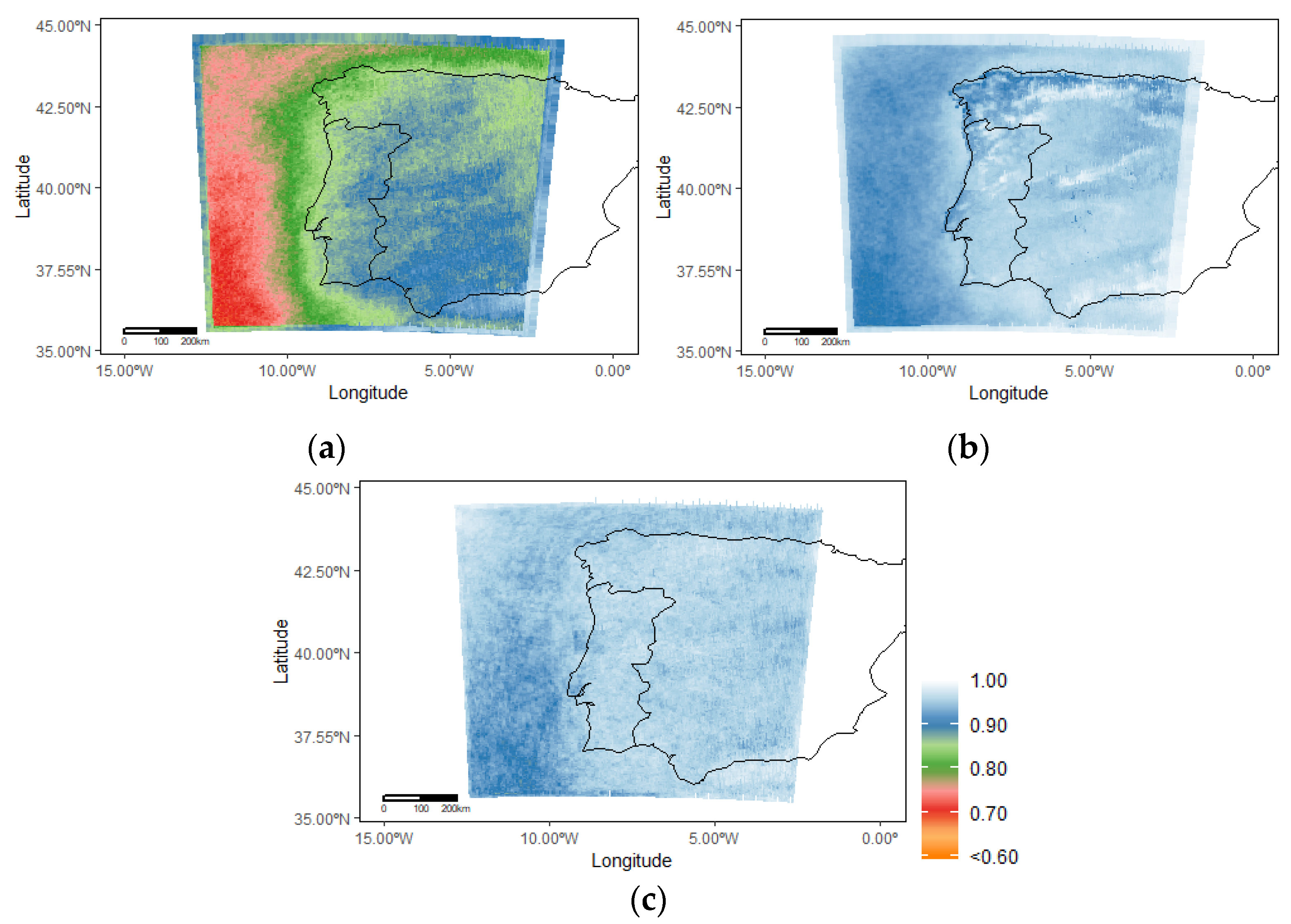
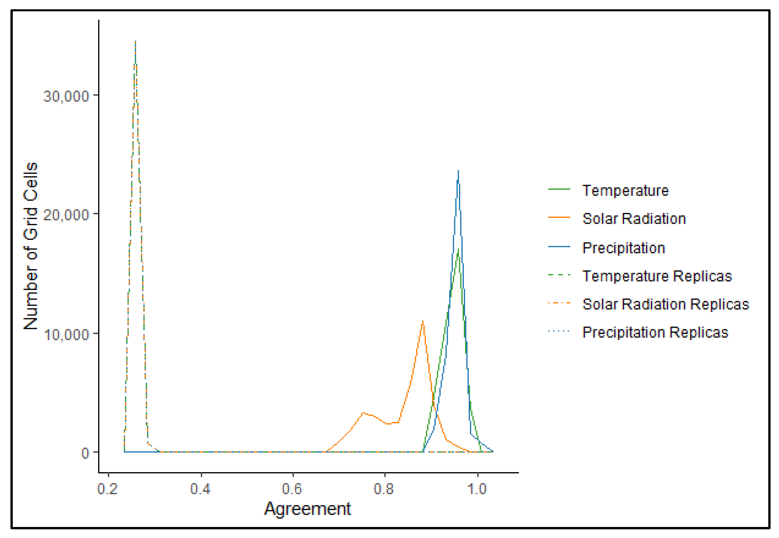
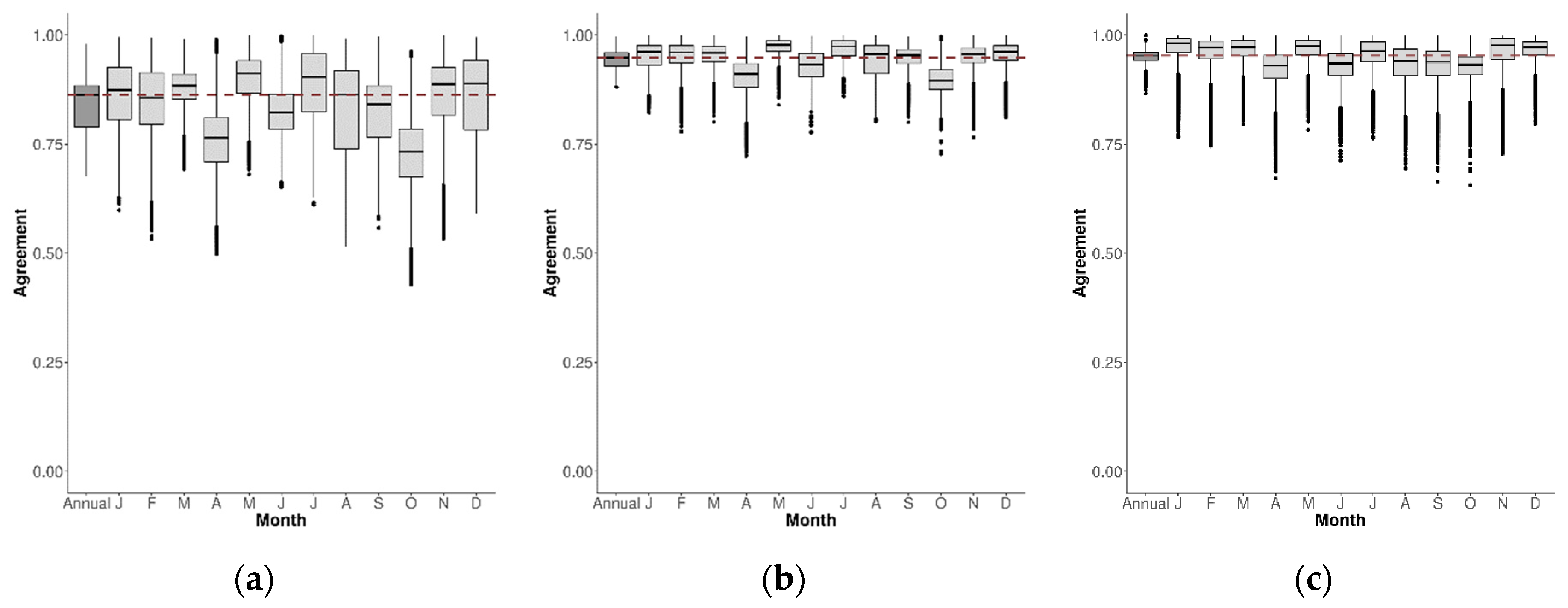
4. Direct and Semi-Direct Aerosol Effects on Meteorology

In this section, the statistical and spatial variability of the meteorological variables considering the two WRF-Chem simulations (with and without aerosol feedback) are presented and discussed.
Figure 2 shows the spatial distribution of agreement for the set of meteorological variables.
Air temperature and precipitation have agreement values ranging from 0.87 up to 1.00, while solar radiation presents lower agreement, varying between 0.68 and 0.98. Solar radiation agreement is lower over the ocean (0.68–0.75) comparatively to land regions (0.75–0.98), probably due to ocean-land differences based on the extent, height and type of clouds and their interaction with the atmospheric aerosol. Thereby, the higher variability over the ocean comparing both simulations is largely associated with the approach used for quantifying semi-direct aerosol effects, since its influence on the radiative forcing induces changes in other meteorological variables (surface temperature, relative humidity, wind speed) impacting the cloud cover [11,12,13,16,60].
The distribution of the number of grid cells per agreement value for each meteorological variable considering the original data and the mean of the bootstrap replicas is presented in Figure 3.
With regards to temperature and precipitation, the very small spatial differences in Figure 2 resulted in similar distribution curves of agreement ( A ). In turn, solar radiation has a distinct behaviour, presenting a bimodal distribution curve with a mode approximately at 0.75, and another close to 0.87. The lowest mode describes the distribution of agreement values for ocean regions (lower agreement values), while the higher mode is characteristic of the agreement distribution over land regions. Bootstrap analysis for each meteorological variable revealed that agreement values were statistically significant for all grid cells. In fact, mean distributions of bootstrap replicas are quite distinct from the original data. Furthermore, agreement values, when there is no cross-spectral density, have a mean A value around 0.25. In the case of precipitation, the 756 grid cells in the outer layer have time series entirely composed of zeros. Therefore, shuffling these time series is pointless as agreement will always be one. Consequently, these grid cells are not included in the mean distribution of replicas, nor are they considered in the statistical analysis. It must be noted that precipitation is influenced by semi-direct and indirect aerosol effects [30,33,45], and that the latter were not considered in this study. Indirect aerosol effects are more relevant than radiative effects in altering the cloud properties and precipitation [13,16,24].
By analysing the monthly variation of agreement values, it is possible to observe that once again solar radiation (Figure 4a) exhibits larger variability than temperature and precipitation (Figure 4b,c).
For all meteorological variables, agreement values in April, June and October are lower compared to the annual average agreement. One-way analysis of variance (ANOVA) was used to test whether all monthly averages were equal to the annual average and, statistically significant differences (at 5% significance level) from the annual mean were found ( p = 10 5 ) . Several reasons might justify the larger variability during these months: higher shortwave radiation, increased biogenic emissions leading to the formation of secondary organic aerosol, more dynamic ABL, or even predominance of particles due to Saharan dust episodes and agricultural activities [6,38,61].
To complement this analysis, mean coherence profiles for the solar radiation and temperature were constructed, including two distinct groups: i) one for the months with median agreement lower than the annual agreement (April, June and October); and ii) the other group with the remaining months (Figure 5).
As expected, both meteorological variables present lower mean coherence values for the months with lower median agreement. Nevertheless, the mean coherence is not constant across frequencies and shows a decreasing pattern with increasing frequency. This result indicates that the time series based on modelled values are more similar in terms of the overall monthly trend ( f < 0.01 ), while the largest differences are observed in very short periods of time ( f = 0.5 corresponding to episodes of 2 h). The decrease observed in the coherence function is greater for the solar radiation, which is in accordance with the previous results.
Besides the statistical analysis, annual mean and maximum spatial differences between simulations (with feedback and without feedback) for the solar radiation (Figure 6) and air temperature (Figure 7) are also presented.
Looking at the solar radiation maps, higher mean values were estimated when the aerosol feedback was neglected, mainly over ocean regions (negative differences in Figure 6a). This radiation variability (up to 20 Wm−2) is associated to the methodological assumptions used for estimating aerosol effects (direct and semi-direct) and their relationship with the aerosol optical properties, as well as to spatial and vertical distribution of both aerosol and cloud layers. Therefore, overall, the aerosol feedback favoured the scattering and absorption of the shortwave and longwave radiation into the atmosphere (direct effect), leading to its warming and subsequent decrease of the amount of solar energy that reaches the ground surface. On the other hand, the higher differences over the ocean, which resulted in a lower agreement (Figure 2a), could be related with the aerosol–cloud dynamics (semi-direct effect), since the cloud physical characteristics (e.g., geometry, water content, particles size) significantly differ between land and sea, influencing the Earth-atmosphere radiative energy budget [11,17,19,25,62]. Similar spatial pattern and the same sign of the mean radiation was found when mapping the maximum solar radiation differences (up to 40 Wm−2) (Figure 6b).
Regarding the impact of solar radiation on the air temperature near the surface, very small differences were estimated (up to 0.5 °C) (Figure 7).
On land, as expected, the used aerosol schemes contributed to a slight decrease of both solar radiation and temperature, whereas on the ocean the aerosol had the opposite effect on the meteorological variables; that is, the largest radiation reduction led to a very small increase of the surface temperature. These solar radiation and air temperature variations, related with the direct aerosol effect, especially those estimated on land surfaces, are in the range of other studies using WRF-Chem over Europe (e.g., [6,12,15,17]).
However, the analysis of these results should be viewed with some caution, since the MADE/SORGAM aerosol module concerning the used dust and sea-salt options (dust_opt = 2; seas_opt = 2) was disabled in WRF-Chem versions later than 3.6.1, due to errors in the aerosol schemes [41]. Notwithstanding these reported bugs, to take into account in new studies and/or to complement this research, it is important to note that the combination of these options was accepted or even recommended until the WRF-Chem version 3.6.1, modelling system was adopted in the present work.

5. Summary and Conclusions

This study aimed to investigate the direct and semi-direct aerosol effects on the weather forecast using the online WRF-Chem model. For this purpose, two WRF-Chem simulations focused on the Iberian Peninsula domain, with and without aerosol feedback, were performed for the year 2015. Agreement metrics were used to evaluate the importance of the aerosol radiative effect on the major meteorological variables (shortwave radiation, air temperature and precipitation), and a bootstrap analysis was done to check for statistical significance of the results.
Annual average agreement for temperature and precipitation showed that both simulations behave similarly in terms of spatial distribution (0.87–1.00). In contrast, solar radiation has lower values and larger variability of agreement (0.68–0.98), mainly over the ocean. Furthermore, for all meteorological variables, a temporal variation with lower agreement values in April, June and October is observed. The inclusion of the aerosol feedback resulted in most significant absolute differences for the solar radiation (up to 20 and 40 Wm−2 for annual mean and maximum values), while the temperature near the surface (2 m) had a slight oscillation (up to 0.5 °C). To identify and understand these differences, a more comprehensive analysis regarding the radiation and heat transfer processes, atmospheric boundary layer dynamics and presence of natural sources of atmospheric aerosols (e.g., mineral dust and sea-salt) and their online calculation methods need to be accomplished, in order to select the most appropriate aerosol schemes for the region of interest. Besides the direct aerosol effects studied here, further research to improve the numerical representation of the clouds and their interaction with the aerosols and radiation (i.e., indirect aerosol effects) should be carried out.
In general, the presented results demonstrate and confirm that the aerosol particles can play a significant role in the atmosphere–Earth dynamics, influencing the net radiation budget and underlying meteorological conditions. Thereby, for future research works, it is recommended to account for the aerosol effect (direct and indirect) when performing weather predictions, and not only for purposes of air quality assessment, since meteorological models at operational centres are highly tuned to produce the best possible forecast of the meteorological fields. The inclusion of these effects will imply, however, additional computation effort that needs to be assessed to not compromise the prognostic service.

Author Contributions

Conceptualization, C.S., A.M. (Ana Martins), S.G. and A.M. (Alexandra Monteiro); methodology, C.S., A.M. (Ana Martins), S.G. and A.M. (Alexandra Monteiro); software, C.S. and A.M. (Ana Martins).; validation, C.S., A.M. (Ana Martins)., S.G. and A.M. (Alexandra Monteiro); formal analysis, C.S., A.M. (Ana Martins), S.G. and A.M. (Alexandra Monteiro); investigation, C.S. and A.M. (Ana Martins).; writing—original draft preparation, C.S., A.M. (Ana Martins). and A.M. (Alexandra Monteiro); writing—review and editing, C.S., A.M. (Ana Martins), S.G., M.S., A.I.M. and A.M. (Alexandra Monteiro); supervision, S.G., A.I.M. and A.M. (Alexandra Monteiro). All authors have read and agreed to the published version of the manuscript.

Funding

The authors would like to thank the Paolo Tuccella and Gabriele Curci for providing the anthropogenic emissions processing interface. Thanks are also due to FCT/MCTES for the financial support to CESAM (UIDP/50017/2020+UIDB/50017/2020), through national funds. Carlos Silveira acknowledges the FCT PhD grant ref. SFRH/BD/112343/2015. Ana Martins acknowledges the individual financial support through IEETA I&D funding UID/CEC/00127/2019 and the FCT PhD grant ref. SFRH/BD/143973/2019.

Institutional Review Board Statement

Not applicable.

Informed Consent Statement

Not applicable.

Data Availability Statement

Publicly available datasets were analyzed in this study.

Conflicts of Interest

The authors declare no conflict of interest.

References

  1. Baklanov, A.; Schlünzen, K.; Suppan, P.; Baldasano, J.; Brunner, D.; Aksoyoglu, S.; Carmichael, G.; Douros, J.; Flemming, J.; Forkel, R.; et al. Online coupled regional meteorology chemistry models in Europe: Current status and prospects. Atmos. Chem. Phys. 2014, 14, 317–398. [Google Scholar] [CrossRef] [Green Version]
  2. Grell, G.; Baklanov, A. Integrated modeling for forecasting weather and air quality: A call for fully coupled approaches. Atmos. Environ. 2011, 45, 6845–6851. [Google Scholar] [CrossRef]
  3. Inness, P.; Dorling, S. Operational Weather Forecasting; John Wiley & Sons, Ltd.: Chichester, UK, 2012; ISBN 9781118447659. [Google Scholar]
  4. Wang, J.; Allen, D.J.; Pickering, K.E.; Li, Z.; He, H. Impact of aerosol direct effect on East Asian air quality during the EAST-AIRE campaign. J. Geophys. Res. Atmos. 2016, 121, 6534–6554. [Google Scholar] [CrossRef] [Green Version]
  5. Chen, F.; Kusaka, H.; Bornstein, R.; Ching, J.; Grimmond, C.S.B.; Grossman-Clarke, S.; Loridan, T.; Manning, K.W.; Martilli, A.; Miao, S.; et al. The integrated WRF/urban modelling system: Development, evaluation, and applications to urban environmental problems. Int. J. Climatol. 2011, 31, 273–288. [Google Scholar] [CrossRef]
  6. Werner, M.; Kryza, M.; Skjøth, C.A.; Wałaszek, K.; Dore, A.J.; Ojrzyńska, H.; Kapłon, J. Aerosol-Radiation Feedback and PM10 Air Concentrations Over Poland. Pure Appl. Geophys. 2017, 174, 551–568. [Google Scholar] [CrossRef] [Green Version]
  7. Zhang, Y. Online-coupled meteorology and chemistry models: History, current status, and outlook. Atmos. Chem. Phys. 2008, 8, 2895–2932. [Google Scholar] [CrossRef] [Green Version]
  8. Vautard, R.; Moran, M.D.; Solazzo, E.; Gilliam, R.C.; Matthias, V.; Bianconi, R.; Chemel, C.; Ferreira, J.; Geyer, B.; Hansen, A.B.; et al. Evaluation of the meteorological forcing used for the Air Quality Model Evaluation International Initiative (AQMEII) air quality simulations. Atmos. Environ. 2012, 53, 15–37. [Google Scholar] [CrossRef] [Green Version]
  9. Korsholm, U.S.; Baklanov, A.; Gross, A.; Sørensen, J.H. On the importance of the meteorological coupling interval in dispersion modeling during ETEX-1. Atmos. Environ. 2009, 43, 4805–4810. [Google Scholar] [CrossRef]
  10. Grell, G.A. Online versus offline air quality modeling on cloud-resolving scales. Geophys. Res. Lett. 2004, 31, L16117. [Google Scholar] [CrossRef]
  11. Thomas, M.A.; Kahnert, M.; Andersson, C.; Kokkola, H.; Hansson, U.; Jones, C.; Langner, J.; Devasthale, A. Integration of prognostic aerosol–cloud interactions in a chemistry transport model coupled offline to a regional climate model. Geosci. Model Dev. 2015, 8, 1885–1898. [Google Scholar] [CrossRef] [Green Version]
  12. Forkel, R.; Balzarini, A.; Baró, R.; Bianconi, R.; Curci, G.; Jiménez-Guerrero, P.; Hirtl, M.; Honzak, L.; Lorenz, C.; Im, U.; et al. Analysis of the WRF-Chem contributions to AQMEII phase2 with respect to aerosol radiative feedbacks on meteorology and pollutant distributions. Atmos. Environ. 2015, 115, 630–645. [Google Scholar] [CrossRef]
  13. Archer-Nicholls, S.; Lowe, D.; Schultz, D.M.; McFiggans, G. Aerosol–radiation–cloud interactions in a regional coupled model: The effects of convective parameterisation and resolution. Atmos. Chem. Phys. 2016, 16, 5573–5594. [Google Scholar] [CrossRef] [Green Version]
  14. Fast, J.D.; Gustafson, W.I.; Easter, R.C.; Zaveri, R.A.; Barnard, J.C.; Chapman, E.G.; Grell, G.A.; Peckham, S.E. Evolution of ozone, particulates, and aerosol direct radiative forcing in the vicinity of Houston using a fully coupled meteorology-chemistry-aerosol model. J. Geophys. Res. 2006, 111, D21305. [Google Scholar] [CrossRef]
  15. Palacios-Peña, L.; Baró, R.; Guerrero-Rascado, J.L.; Alados-Arboledas, L.; Brunner, D.; Jiménez-Guerrero, P. Evaluating the representation of aerosol optical properties using an online coupled model over the Iberian Peninsula. Atmos. Chem. Phys. 2017, 17, 277–296. [Google Scholar] [CrossRef] [Green Version]
  16. Chapman, E.G.; Gustafson, W.I.; Easter, R.C.; Barnard, J.C.; Ghan, S.J.; Pekour, M.S.; Fast, J.D. Coupling aerosol-cloud-radiative processes in the WRF-Chem model: Investigating the radiative impact of elevated point sources. Atmos. Chem. Phys. 2009, 9, 945–964. [Google Scholar] [CrossRef] [Green Version]
  17. Forkel, R.; Werhahn, J.; Hansen, A.B.; McKeen, S.; Peckham, S.; Grell, G.; Suppan, P. Effect of aerosol-radiation feedback on regional air quality—A case study with WRF/Chem. Atmos. Environ. 2012, 53, 202–211. [Google Scholar] [CrossRef]
  18. Liu, X.-Y.; Zhang, Y.; Zhang, Q.; He, K.-B. Application of online-coupled WRF/Chem-MADRID in East Asia: Model evaluation and climatic effects of anthropogenic aerosols. Atmos. Environ. 2016, 124, 321–336. [Google Scholar] [CrossRef] [Green Version]
  19. San José, R.; Pérez, J.L.; Balzarini, A.; Baró, R.; Curci, G.; Forkel, R.; Galmarini, S.; Grell, G.; Hirtl, M.; Honzak, L.; et al. Sensitivity of feedback effects in CBMZ/MOSAIC chemical mechanism. Atmos. Environ. 2015, 115, 646–656. [Google Scholar] [CrossRef] [Green Version]
  20. Li, Z.; Xue, H.; Yang, F. A modeling study of ice formation affected by aerosols. J. Geophys. Res. Atmos. 2013, 118, 11213–11227. [Google Scholar] [CrossRef]
  21. Fan, J.; Wang, Y.; Rosenfeld, D.; Liu, X. Review of aerosol-cloud interactions: Mechanisms, significance, and challenges. J. Atmos. Sci. 2016, 73, 4221–4252. [Google Scholar] [CrossRef]
  22. Glotfelty, T.; Zhang, Y.; Karamchandani, P.; Streets, D.G. Changes in future air quality, deposition, and aerosol-cloud interactions under future climate and emission scenarios. Atmos. Environ. 2016, 139, 176–191. [Google Scholar] [CrossRef] [Green Version]
  23. Brunner, D.; Savage, N.; Jorba, O.; Eder, B.; Giordano, L.; Badia, A.; Balzarini, A.; Baró, R.; Bianconi, R.; Chemel, C.; et al. Comparative analysis of meteorological performance of coupled chemistry-meteorology models in the context of AQMEII phase 2. Atmos. Environ. 2015, 115, 470–498. [Google Scholar] [CrossRef]
  24. Zhang, B.; Wang, Y.; Hao, J. Simulating aerosol–radiation–cloud feedbacks on meteorology and air quality over eastern China under severe haze conditions in winter. Atmos. Chem. Phys. 2015, 15, 2387–2404. [Google Scholar] [CrossRef] [Green Version]
  25. Zhang, Y.; Karamchandani, P.; Glotfelty, T.; Streets, D.G.; Grell, G.; Nenes, A.; Yu, F.; Bennartz, R. Development and initial application of the global-through-urban weather research and forecasting model with chemistry (GU-WRF/Chem). J. Geophys. Res. Atmos. 2012, 117. [Google Scholar] [CrossRef] [Green Version]
  26. Cai, C.; Zhang, X.; Wang, K.; Zhang, Y.; Wang, L.; Zhang, Q.; Duan, F.; He, K.; Yu, S.-C. Incorporation of new particle formation and early growth treatments into WRF/Chem: Model improvement, evaluation, and impacts of anthropogenic aerosols over East Asia. Atmos. Environ. 2016, 124, 262–284. [Google Scholar] [CrossRef] [Green Version]
  27. Zhang, Y.; Zhang, X.; Wang, K.; Zhang, Q.; Duan, F.; He, K. Application of WRF/Chem over East Asia: Part II. Model improvement and sensitivity simulations. Atmos. Environ. 2016, 124, 301–320. [Google Scholar] [CrossRef] [Green Version]
  28. Kong, X.; Forkel, R.; Sokhi, R.S.; Suppan, P.; Baklanov, A.; Gauss, M.; Brunner, D.; Barò, R.; Balzarini, A.; Chemel, C.; et al. Analysis of meteorology–chemistry interactions during air pollution episodes using online coupled models within AQMEII phase-2. Atmos. Environ. 2015, 115, 527–540. [Google Scholar] [CrossRef]
  29. Zhang, Y.; Sartelet, K.; Zhu, S.; Wang, W.; Wu, S.-Y.; Zhang, X.; Wang, K.; Tran, P.; Seigneur, C.; Wang, Z.-F. Application of WRF/Chem-MADRID and WRF/Polyphemus in Europe—Part 2: Evaluation of chemical concentrations and sensitivity simulations. Atmos. Chem. Phys. 2013, 13, 6845–6875. [Google Scholar] [CrossRef] [Green Version]
  30. Park, S.-Y.; Lee, H.-J.; Kang, J.-E.; Lee, T.; Kim, C.-H. Aerosol radiative effects on mesoscale cloud–precipitation variables over Northeast Asia during the MAPS-Seoul 2015 campaign. Atmos. Environ. 2018, 172, 109–123. [Google Scholar] [CrossRef]
  31. Saide, P.E.; Spak, S.N.; Carmichael, G.R.; Mena-Carrasco, M.A.; Yang, Q.; Howell, S.; Leon, D.C.; Snider, J.R.; Bandy, A.R.; Collett, J.L.; et al. Evaluating WRF-Chem aerosol indirect effects in Southeast Pacific marine stratocumulus during VOCALS-REx. Atmos. Chem. Phys. 2012, 12, 3045–3064. [Google Scholar] [CrossRef] [Green Version]
  32. Tuccella, P.; Curci, G.; Crumeyrolle, S.; Visconti, G. Modeling of Aerosol Indirect Effects with WRF/Chem over Europe. In Air Pollution Modeling and Its Application XXIII; Springer: Cham, Switzerland, 2014; pp. 91–95. [Google Scholar]
  33. Yang, Q.; Gustafson, W.I.; Fast, J.D.; Wang, H.; Easter, R.C.; Wang, M.; Ghan, S.J.; Berg, L.K.; Leung, L.R.; Morrison, H. Impact of natural and anthropogenic aerosols on stratocumulus and precipitation in the Southeast Pacific: A regional modelling study using WRF-Chem. Atmos. Chem. Phys. 2012, 12, 8777–8796. [Google Scholar] [CrossRef] [Green Version]
  34. Soupiona, O.; Papayannis, A.; Kokkalis, P.; Foskinis, R.; Sánchez Hernández, G.; Ortiz-Amezcua, P.; Mylonaki, M.; Papanikolaou, C.-A.; Papagiannopoulos, N.; Samaras, S.; et al. EARLINET observations of Saharan dust intrusions over the northern Mediterranean region (2014–2017): Properties and impact on radiative forcing. Atmos. Chem. Phys. 2020, 20, 15147–15166. [Google Scholar] [CrossRef]
  35. Salvador, P.; Barreiro, M.; Gómez-Moreno, F.J.; Alonso-Blanco, E.; Artíñano, B. Synoptic classification of meteorological patterns and their impact on air pollution episodes and new particle formation processes in a south European air basin. Atmos. Environ. 2021, 245, 118016. [Google Scholar] [CrossRef]
  36. Grell, G.A.; Peckham, S.E.; Schmitz, R.; McKeen, S.A.; Frost, G.; Skamarock, W.C.; Eder, B. Fully coupled “online” chemistry within the WRF model. Atmos. Environ. 2005, 39, 6957–6975. [Google Scholar] [CrossRef]
  37. WMO. WMO Statement on the Status of the Global Climate in 2015; WMO-No. 11; World Meteorological Organization: Geneva, Switzerland, 2016; ISBN 978-92-63-11167-8. [Google Scholar]
  38. EEA. Air Quality in Europe—2019 Report; EEA: Copenhagen, Denmark, 2019; ISBN 978-92-9480-088-6. [Google Scholar]
  39. Kuik, F.; Lauer, A.; Churkina, G.; Denier van der Gon, H.A.C.; Fenner, D.; Mar, K.A.; Butler, T.M. Air quality modelling in the Berlin–Brandenburg region using WRF-Chem v3.7.1: Sensitivity to resolution of model grid and input data. Geosci. Model Dev. 2016, 9, 4339–4363. [Google Scholar] [CrossRef] [Green Version]
  40. National Center for Atmospheric Research (NCAR) WRF Model Users’ Page. Available online: https://www2.mmm.ucar.edu/wrf/users/ (accessed on 2 February 2021).
  41. National Oceanic and Atmospheric Administration (NOAA) Weather Research and Forecasting Model Coupled to Chemistry (WRF-Chem)—User Support. Available online: https://ruc.noaa.gov/wrf/wrf-chem/user-support.htm (accessed on 2 February 2021).
  42. Pineda, N.; Jorba, O.; Jorge, J.; Baldasano, J.M. Using NOAA AVHRR and SPOT VGT data to estimate surface parameters: Application to a mesoscale meteorological model. Int. J. Remote Sens. 2004, 25, 129–143. [Google Scholar] [CrossRef]
  43. Tuccella, P.; Curci, G.; Visconti, G.; Bessagnet, B.; Menut, L.; Park, R.J. Modeling of gas and aerosol with WRF/Chem over Europe: Evaluation and sensitivity study. J. Geophys. Res. Atmos. 2012, 117. [Google Scholar] [CrossRef] [Green Version]
  44. NCAR WRF-Chem Tools for the Community. Available online: https://www2.acom.ucar.edu/wrf-chem/wrf-chem-tools-community (accessed on 26 April 2019).
  45. Cardoso, R.M.; Soares, P.M.M.; Miranda, P.M.A.; Belo-Pereira, M. WRF high resolution simulation of Iberian mean and extreme precipitation climate. Int. J. Climatol. 2013, 33, 2591–2608. [Google Scholar] [CrossRef]
  46. Marta-Almeida, M.; Teixeira, J.C.; Carvalho, M.J.; Melo-Gonçalves, P.; Rocha, A.M. High resolution WRF climatic simulations for the Iberian Peninsula: Model validation. Phys. Chem. Earth Parts A/B/C 2016, 94, 94–105. [Google Scholar] [CrossRef]
  47. Baró, R.; Palacios-Peña, L.; Baklanov, A.; Balzarini, A.; Brunner, D.; Forkel, R.; Hirtl, M.; Honzak, L.; Pérez, J.L.; Pirovano, G.; et al. Regional effects of atmospheric aerosols on temperature: An evaluation of an ensemble of online coupled models. Atmos. Chem. Phys. 2017, 17, 9677–9696. [Google Scholar] [CrossRef] [Green Version]
  48. Kay, S.M. Modern Spectral Estimation: Theory and Application; Prentice Hall: Englewood Cliffs, NJ, USA, 1988; ISBN 013598582X. [Google Scholar]
  49. R Core Team. R: A Language and Environment for Statistical Computing. R Foundation for Statistical Computing. Available online: http://www.r-project.org (accessed on 2 February 2021).
  50. Pierce, D. ncdf4: Interface to Unidata netCDF (Version 4 or Earlier) Format Data Files. Available online: https://cran.r-project.org/web/packages/ncdf4/ (accessed on 2 February 2021).
  51. Bronaugh, D. ncdf4.helpers: Helper Functions for Use with the “ncdf4” Package. Available online: CRAN.R-project.org/package=ncdf4.helpers (accessed on 2 February 2021).
  52. Sueur, J.; Aubin, T.; Simonis, C. Seewave, a free modular tool for sound analysis and synthesis. Bioacoustics 2008, 18, 213–226. [Google Scholar] [CrossRef]
  53. Borchers, H.W. pracma: Practical Numerical Math Functions. Available online: https://cran.r-project.org/package=pracma (accessed on 2 February 2021).
  54. Wickham, H. ggplot2: Elegant Graphics for Data Analysis; Springer: New York, NY, USA, 2016. [Google Scholar]
  55. Deckmyn, A. maps: Draw Geographical Maps. Available online: https://cran.r-project.org/package=maps (accessed on 2 February 2021).
  56. Bivand, R.; Lewin-Koh, N.; Pebesma, E.; Archer, E. Maptools: Tools for Handling Spatial Objects. Available online: https://cran.r-project.org/package=maptools (accessed on 2 February 2021).
  57. Pebesma, E.; Bivand, R.S. Classes and Methods for Spatial Data: The sp Package. R News 2005, 5, 9–13. Available online: https://CRAN.R-project.org/doc/Rnews/ (accessed on 2 February 2021).
  58. Baquero, O.S. ggsn: North Symbols and Scale Bars for Maps Created with “ggplot2” or “ggmap”. Available online: https://cran.r-project.org/web/packages/ggsn/ (accessed on 2 February 2021).
  59. Garnier, S.; Ross, N.; Rudis, B.; Sciaini, M.; Scherer, C. viridis: Default Color Maps from “matplotlib”. Available online: https://cran.r-project.org/package=viridis (accessed on 2 February 2021).
  60. Briant, R.; Tuccella, P.; Deroubaix, A.; Khvorostyanov, D.; Menut, L.; Mailler, S.; Turquety, S. Aerosol–radiation interaction modelling using online coupling between the WRF 3.7.1 meteorological model and the CHIMERE 2016 chemistry-transport model, through the OASIS3-MCT coupler. Geosci. Model Dev. 2017, 10, 927–944. [Google Scholar] [CrossRef] [Green Version]
  61. Sporre, M.K.; Blichner, S.M.; Karset, I.H.H.; Makkonen, R.; Berntsen, T.K. BVOC–aerosol–climate feedbacks investigated using NorESM. Atmos. Chem. Phys. 2019, 19, 4763–4782. [Google Scholar] [CrossRef] [Green Version]
  62. Chen, D.; Liu, Z.; Davis, C.; Gu, Y. Dust radiative effects on atmospheric thermodynamics and tropical cyclogenesis over the Atlantic Ocean using WRF-Chem coupled with an AOD data assimilation system. Atmos. Chem. Phys. 2017, 17, 7917–7939. [Google Scholar] [CrossRef] [Green Version]
Figure 1. Weather Research and Forecasting (WRF)-Chem simulation domains.
Atmosphere 12 00288 g001
Figure 2. Spatial variability of agreement ( A ) between the WRF-Chem simulations, with and without aerosol feedback, for the analysed meteorological variables: (a) solar radiation; (b) air temperature; and (c) precipitation.
Atmosphere 12 00288 g002
Figure 3. Agreement ( A ) distributions for all meteorological variables. Solid lines represent the distribution of the agreement values for the 36,000 grid cells of the original data, while dotted lines show the distribution of the average agreement of the bootstrap replicas (B = 10) for each grid cell and for each variable.
Atmosphere 12 00288 g003
Figure 4. Distribution of agreement ( A ) between the WRF-Chem simulations, with and without aerosol feedback, for the analysed meteorological variables: (a) solar radiation; (b) air temperature; and (c) precipitation. The first box represents annual agreement values and the remaining represent monthly ones. Each box includes the agreement obtained for the 36,000 grid cells, and it is delimited by the 25th and 75th percentiles and the middle line representing the 50th percentile of the distribution of the agreement. The threshold for outliers’ identification (black dots) is based on 1.5 times the interquartile range. Red dashed line shows the median of the annual agreement.
Atmosphere 12 00288 g004
Figure 5. Mean coherence profile for the (a) solar radiation and (b) air temperature. Blue line represents the mean coherence profile of the lower median agreement months, while the purple line shows the mean coherence profile for the remaining months.
Atmosphere 12 00288 g005
Figure 6. Spatial differences of solar radiation comparing both simulations (with feedback and without feedback): (a) annual average including all hourly values; and (b) annual average of daily maximum values.
Atmosphere 12 00288 g006
Figure 7. Spatial differences of air temperature comparing both simulations (with feedback and without feedback): (a) annual average including all hourly values; and (b) annual average of daily maximum values.
Atmosphere 12 00288 g007
Table 1. Main physical and chemical parametrizations used in the WRF-Chem simulations.
ProcessesOption 1Remarks
MicrophysicsMorrison double-moment
Short-wave radiationRRTMGCalled every 25 min
Long-wave radiationRRTMGCalled every 25 min
Surface layerMonin–Obukhov Similarity
Land-surface modelNCEP Noah LSM33-classes land cover
Boundary-layer schemeMYNN 2.5 level TKE
CumulusGrell 3D
PhotolysisFast-J
Gas-phase mechanismRADM2Fixed version (chem_opt = 2)
Aerosol moduleMADE/SORGAM
Aerosol-radiation feedback turned on or offDirect and semi-direct effects
Aerosol optical propertiesVolume approximation
1 The methodological assumptions of these options are described in the WRF and WRF-Chem users’ support websites [40,41]. Acronyms: RRTMG—Rapid Radiative Transfer Model for General Circulation Models; NCEP Noah—National Center for Environmental Prediction; LSM—Land Surface Model; MYNN—Mellor–Yamada–Nakanishi–Niino; TKE—Turbulent Kinetic Energy; RADM2—Regional Acid Deposition Model, 2nd generation; MADE/SORGAM—Modal Aerosol Dynamics Model for Europe/Secondary Organic Aerosol Model.
Publisher’s Note: MDPI stays neutral with regard to jurisdictional claims in published maps and institutional affiliations.

