Article

Trends of Aerosol Optical Thickness Using VIIRS S-NPP during Fog Episodes in Pakistan and India

1
Institute of Geographical Information System (IGIS), National University of Science and Technology (NUST), Islamabad 44000, Pakistan
2
Department of Geography, Southern Illinois University Edwardsville, Edwardsville, IL 62026, USA
3
Institute of Environmental Sciences and Engineering (IESE), National University of Sciences and Technology, Islamabad 44000, Pakistan
*
Author to whom correspondence should be addressed.
Atmosphere 2021, 12(2), 242; https://doi.org/10.3390/atmos12020242
Submission received: 7 December 2020 / Revised: 30 January 2021 / Accepted: 4 February 2021 / Published: 11 February 2021
(This article belongs to the Special Issue Aerosol Pollution in Asia)

Abstract

:
Aerosol Optical Thickness (AOT) is one of the important parameters for assessing regional and global level of climate change. Fog episodes have considerably increased in south Asia because of environmental factors, and the burning of agricultural residue leads to major social and economic problems. In present study, Mann-Kendall trend analysis of AOT and active fire events was done, and their significance were assessed using long-term (October 2012–February 2020) remote sensing data derived smog maps. Visible Infrared Imaging Radiometer Suite National Polar Partnership (VIIRS N-PP) was used to map AOT episodes over the northern region of Pakistan and India. Results reveal that AOT displays a significantly decreasing trend over the northern and eastern region of Pakistan and a similar decreasing trend from the Western to Eastern region of India. Furthermore, active fire events have a significantly increasing trend at the Northern region of Pakistan. However, fire events have a significantly decreasing trend over the southern and southeastern region of India. Additionally, statistically significant decreasing trends were observed for AOT over Chakwal (p-value = 0.2, Z_MK = −2.3) and Patiala (p-value = 0.15, Z_MK = −3.2). Fire events have a significantly increasing trend for Dera Ismail Khan (p-value = 0.01, Z_MK = 1.9), Jhang (p-value = 0.01, Z_MK = 1.9), and Chakwal (p-value = 0.01, Z_MK = 1.8), while they are significantly decreasing trend near New Delhi (p-value = 0.2, Z_MK = −0.9), Aligarh (p-value = 0.15, Z_MK = −0.9) and Patiala (p-value = 0.2, Z_MK = −0.8).

1. Introduction

Atmospheric aerosols are an important constituent of the atmosphere and have direct influence on climate, weather, and human health [1]. Aerosol Optical Thickness (AOT) is used to assess information about the quantity of aerosols as it shows how much light is lost along the vertical columns of the atmosphere. Atmospheric aerosols not only trigger local phenomena but also influence the regional atmosphere [2]. Aerosols are already pervasive across South Asia because of air pollution caused by urbanization [3]. Aerosols also affect the hydrological cycle and atmospheric chemistry [4,5] as well as human health [6]. Their natural sources include volcanic ash, sea salt spray, and dust storms. Aerosols are heavily influenced by the human-made activities such as transportation, industrialization, and the burning of agricultural biomass [7,8]. Aerosols particles also reduce the visibility and are perceptible through haze, dust, and smoke [9]. Furthermore, emissions from the burning of fossils fuels from November to January are a common phenomenon in South Asia as the burning of crop residue is an easy, fast, and inexpensive way to clear agricultural fields [10,11,12,13,14,15]. Haze is an air pollutant that is triggered by large aerosols [16]. Its formation is related to particles emitted from anthropogenic sources under favorable meteorological conditions (i.e., weak wind speed and high humidity) [17]. During the last couple of decades there have been cases of regional haze occurring in the eastern part of Punjab in Pakistan and northwestern part of India [18,19]. Historically, data derived from satellites have been used to monitor aerosols. In 1975, a first attempt was made for deriving aerosol products from Landsat sensors [8,20]. For the retrieval of long-term global aerosols products, satellites used are Moderate Resolution Imaging Spectroradiometer (MODIS) [8,21,22,23,24], Multiangle Imaging Spectroradiometer (MISR), Total Ozone Mapping Spectrometer (TOMS), Advanced Very High-Resolution Radiometer (AVHRR) [25] and Visible Infrared Imaging Suite (VIIRS) sensor on board with Suomi National Polar Orbiting Partnership (S-NPP) [26].
Spatial and temporal distribution of aerosols have the significant uncertainty because of its complex physical and chemical properties [27]. However, to minimize the uncertainty correlation of remote sensing data with ground data were anticipated like Huang et al. [28] determined the uncertainty and accuracy of VIIRS product with Aerosol Robotic Network (AERONET), seasonal and regional factor were also incorporated; observed accuracy, precision uncertainty and correlation coefficient of 0.0415, 0.155, 0.16 and 0.741. It was also noticed that daily timeseries of AOT had most significant variability over eastern India with strong negative bias during the spring season when that region has the harvesting season and agricultural biomass burning was occurring at very-large scale.
Meng et al. [29] discovered that AOT550 accessed from AERONET sun-photometer brings out good agreement (high correlation of 0.907, accuracy −0.058 and precision of 0.192) with AOT550 derived from VIITS IP. Moreover, regional differences were also explained in VIIRS IP over south and north china and observed the minor uncertainty difference of 0.195 verse 0.174.
Meng et al. [29] showed that VIIRS Suomi NPP gives quality results while retrieving global aerosol optical thickness (AOT) data at M-band pixel 550 nm (VIIRS) than MODIS. VIIRS exhibits better accuracy and precision because of its large swath size (~3000 km) and presence of a Day-Night Band (DNB) that facilitates the monitoring and regional extent of small-to-large events that influence human health [26,30]
The focus of this study is the spatial and temporal variations of AOT and fire events over cities located in northeastern Pakistan and neighboring India. To date, these have not been examined in tandem utilizing satellite data. For this purpose, AOT affected districts from northern Punjab in Pakistan and India were selected. The selected districts are also high in agricultural production and subsequent crop residue burning practices. This was cross checked using Normalized Difference Vegetation Index (NDVI) timeseries maps. (See Figure 1).

2. Materials and Methods

2.1. Material

In the current study, two different types of remotely sensed datasets were used. Data from the Suomi National Polar Orbiting Partnership (SNPP) Visible Infrared Imaging Radiometer Suite (VIIRS) was acquired for AOT mapping. It is considered a successor for the Sea-viewing Wide Field-of-view Sensor (SeaWIFS), Advanced Very High-Resolution Radiometer (AVHRR), and the Moderate Resolution Imaging Spectroradiometer (MODIS). It was launched in October 2011. It has 22 imaging and radiometry bands, with a swath size of 3060 km, and a spectral range of 0.402 to 12.488 µm [31]. As aerosols have significant influences on major climatological processes, aerosol optical thickness (AOT) was acquired from VIIRS SNPP’s ‘Deep Blue’ data set (AERDB). This dataset consists of daily gridded aggregated data, and it is derived from a primary level-2 dataset at 550 nanometers (nm) using specific bands with the spatial resolution of 1° × 1° of horizontal grid [32]. This dataset was acquired from LAADS DAAC website (of 1st October 2012 to 29th February 2020 (Table 1) [33].
It has been observed that AOT has increased by 40% over several areas of India from 2000 to 2009 due to an increase in urbanization, the burning of biomass and fossil fuels, and forest fires [34]. The residue burning is used as a means to clear agricultural fields [35]. The counts of residue burning can be mapped from satellite remote sensing, fire event data. Near real-time SNPP VIIRS fire event data (i.e., VNP14IMGTDL_NRT) was acquired from National Aeronautics and Space Administration’s (NASA) Fire Information for Resource Management System (FIRMS) Near Real-Time (NRT) site [36]. This dataset was originally prepared as a continuation of the MODIS active fire data [37]. I-band (375 m) and M-band (750 m) VIIRS satellite data were used for active fire detection. It was available from 20th January 2012 to 28th February 2020. The point locations for the fire events of study area were acquired of 1st October 2012 to 28th February 2020 (Table 1).

2.2. Method

Datasets were resampled to the same temporal and spatial resolution to allow for comparative assessment. Fire events data that was initially in temporal resolution of 3 h were aggregated to monthly counts and then transformed from vector to raster. Trend analysis of AOT data was generated by adding the daily values to monthly aggregated raster. All datasets were transformed to similar projection systems and the same spatial resolution (i.e., 9813.43 m.) Each dataset consisted of 176 (11 × 16) cells. Each cell was considered an individual time series. The fog period of October to February for all years was selected for trend analysis [38]. The trend analysis consisted of Lag-1 autocorrelation coefficient ( r 1 ) for the original time series, the Mann-Kendall test for those cells whose values were insignificant at 0.05-level; pre-whitening was done for those cells whose values were significant at 0.05-level before applying the test [39,40,41].
The process of pre-whitening was performed as the significant positive autocorrelation trends showed sufficient increase in its occurrence even when there was no trend [42] and underestimated the likelihood of significant negative autocorrelation trends [43]. Von Storch [42] suggested the process of pre-whitening to eliminate the above case of autocorrelation. So, a new time series x 2 r 1 x 1 ,   x 3 r 1 x 2 ,   . . ,   x n r 1 x 1 1 was calculated and replaced in place of significantly autocorrelated time series [41]. Thus, pre-whitened [43,44] time series were used to identify the statistically significant changes over time The Mann-Kendall test has been used for the identification of time series trends in hydro-climatological data [41,45,46,47,48]. Wang [49] found that non-parametric methods were better when compared to parametric trend determination methods because they are less sensitive to outliers. The Mann-Kendall [50] trend tests the null hypothesis (H0) of time series using rank-based technique and categorized as ‘no trend’, whereas the alternative hypothesis (H1) is categorized as ‘randomness’ (increasing or decreasing trend). The detailed mathematical explanation of Mann-Kendall process along with its formulas is [51,52,53] as follows:
S = k = 1 n 1 j = K + 1 n s g n x j   x k
where:
s g n x j x k =   + 1   i f   X j X k > 0 0         i f   X j X k =   0 1   i f   X j X k <   0
In Equations (1) and (2), n represents the length of time series, x j and x k are the sequential data and S is the Mann-Kendall test statistic. An upward trend is identified by positive value of S and downward trend by negative values. For a long time-series ( n > 10 ), S statistic tends to normality along with expectation E and variance V a r , as follows:
E S = 0
V a r   S = 1 18   n n 1 2 n + 5   p = 1 q t p t p 1 2 t p + 5
In above equation, ‘tp’ is the quantity of observations of ‘pth’ group whereas, the number of tied groups in the time series is denoted by ‘q’. The calculation of standardized test statistic Z M K can be achieved by following equation:
Z M K =   S 1 V a r   S   i f   S > 0 S 1 V a r   S   i f   S < 0 0                           i f   S = 0
The probability-value (p-value) or observed significance level of Mann-Kendall test is related to standard test statistic Z M K , which determines the evidence for null hypothesis. So, positive values of ZMK indicate the increasing trend and negative values of ZMK indicates a decreasing trend. A two-tailed standardized table can be used to obtain the corresponding p-value [53,54].
In the current study, Mann-Kendall trend test was applied to entire datasets. Pre-whitened data was plotted, and linear regression was used for fitting of trend lines using ordinary least square method. Trend analysis of monthly aggregated data was also done for all datasets over major cities of interest in study area. It is believed that increasing episode of haze or smog is related to increasing AOT and fire events.

3. Results and Discussion

Aerosols have been recognized as an important feature that influence global climate change, the water cycle, precipitation and cloud formation, and the atmospheric transformation of thermal and solar radiations [55]. The low sun season in Pakistan (December, January, and February) has been found to be dominated by fog [56]. Smog is common at both dusk and dawn, near industrial and urban areas because of the nocturnal inversion layer. Smog reduces visibility considerably. Smog in Pakistan and northwestern India spreads by western disturbances. However, this type of haze may dissipate when the sun rises and breaks the inversion layer. Additionally, radiation fog is common over northern region of the Himalaya and the Gangetic plain. This type of fog forms low stratus clouds, and persistence time may reach to 2 to 3 days over the Indus Gangetic Plains (IGP) [57].
High levels of air pollution have been noticed over the eastern side of Pakistan. It was reported that the issues of smog in eastern Pakistan, especially around Lahore, started form 2006 and now it has been deemed ‘hazardous’ as the air quality index has increased up to 300 units [58]. Main causes of aerosols in Lahore are biomass burning, emissions from vehicular and industrial activities [59,60]. It was also reported that aerosols formation in Lahore is influenced by transportation of particles generated from the burning of agricultural biomass [12,61,62,63,64]. In winters Lahore’s visibility is limited to 50 m or less [65] causing severe problems for trade and daily commute as well as intercity travel.
Khokhar et al. [66] found the winds that come from India into Pakistan were propagated from the highly inhibited and industrialized parts of Western Uttar Pradesh, New Delhi, Uttarakhand, and Haryana. Likewise, it was determined that burning of agricultural residuals are the primary source of fire over the northern areas of India considerably during the harvesting season of wheat and rice in pre (April and May) and post-monsoon (October and November), respectively [12,13]. As Punjab in India had the residual burning of about 7 to 8 million tons of residual burning during the post-monsoon season [11].
In Delhi, it was determined that the burning of crop residuals and fireworks during Diwali raised the AOT to 30% [61]. For example, northern India has been blanketed with thick pollution for weeks and Delhi has experienced extreme air pollution. In 2015, 4.2 million deaths were recorded because of air pollution and numerous people got ill because of particulate matter in east and south Asia [67].
In this study, the specific time of October to February for 2012–2020 was separated for AOT and fire events for each low sun season. The statistics, such as the Lag–1 autocorrelation coefficient r 1 , was calculated for all monthly aggregated datasets. Altogether, 36 time series (cells) out of 183 were found to be significantly autocorrelated at the 95% significance level ( r 1 value exceeding 0.2); pre-whitening was performed over, and the original time series were replaced by pre-whitened time series (Table 2). p-values displayed the significant (or non-significant) trend of datasets. An insignificant time series is determined with values exceeding 0.2 whereas significant time series is ascertained with values below 0.2 [39,40].
The non-parametric Mann-Kendall trend test was applied for AOT as shown in the trend maps (Figure 2c). Lag-1 autocorrelation coefficient for AOT (Figure 2a) had nine significantly autocorrelated time series, all at the northeastern region of the study area. p-values were calculated for all-time series of AOT to determine trends (Figure 2b). It was determined that AOT has a significantly decreasing trend toward the northern region of Punjab, Pakistan. Similarly, a significantly decreasing trend was also observed at the western to southeastern territory of India covering the province of Haryana, Punjab (India) and Delhi (capital). In addition, a non-significant increasing trend was recorded at the northeastern region of India covering the province of Himachal Pradesh and Kashmir, whereas identical patterns were identified at the northwestern areas (divisions of Sargodha and Dera Ismail khan) of Pakistan as depicted in Figure 2c.
It was recorded that the fire event dataset has twenty-eight significant Lag-1 autocorrelated time series (see Figure 3a); thereafter, significantly autocorrelated time series were replaced by its pre-whitened series substitute. The fire events dataset had a significantly increasing trend over the northern and northwestern region of Pakistan covering the divisions of Sargodha, Rawalpindi, Kohat, Dera Ismail Khan, Faisalabad, and Gujranwala (see Figure 3b,c). In India, there was a significantly decreasing trend observed from the western to southeastern region covering the province of Punjab, Haryana, Delhi, the upper region of Rajasthan and Uttar Pradesh. Conversely, an insignificant increasing trend was witnessed in the northwestern region covering the divisions of Jammu, Kathua, Kangra, Chamba and Kullu (see Figure 3b,c).

AOT Over Urban Areas

Relative time series distribution for each monthly aggregated dataset were also analyzed using for fifteen different cities of Pakistan and India. Autocorrelation coefficient (r), p-value and Mann-Kendall score were also separated for AOT and ’Fire Event’. It was determined that Shimla had the significantly autocorrelated timeseries at 95% significance level for AOT dataset. These time series were per-whitened. It was recorded that Patiala had the significantly (p = 0.15, Z M K = −3.15) decreasing trend with the Kendall score of −119 (Table 3).
It was determined that six cities showed significantly autocorrelated coefficient i.e., New Delhi, Bahawalpur, Dera Ismail Khan, Chamba, Multan and Bahawalnagar for monthly aggregated trend of fire events; pre-whitening was done for these autocorrelated time series and replaced by pre-whitened series. It was noticed that Dera Ismail Khan (p = 0.01, S = 211, Z M K = 1.9), Jhang (p = 0.01, S = 206, Z M K = 1.9) and Chakwal (p = 0.01, S = 196, Z M K = 1.8) had the significantly increasing trend for monthly aggregated trend, whereas Aligarh had the significantly (p = 0.15) decreasing trend with the Kendall score of −98 (Table 4).
AOT were divided into two (1 and 0.5) and determined that high AOT were recorded over the cities of Aligarh, New Delhi, Lahore and Sirsa, whereas Chamba, Gurdaspur, Dera Ismail khan and Shimla had the lowest range of AOT (less than 0.5) and the remaining cities in between 1 and 0.5.
It was also observed that cities located toward the eastern and southern border of Pakistan-India had the decreasing trend for fire events i.e., Lahore and Bahawalpur, whereas Bahawalnagar, Multan, DI-Khan, Chakwal and Jhang had the increasing trend.
It was noticed that AOT starts increasing in the month of October and reached its peak value in November into February (Figure 4). It was observed that Aligarh, New Delhi, Lahore, and Multan have the high AOT during the month of January and February.
Similarly, monthly counts of fire events were also analyzed for all selected cities and it was determined that the number of fire events was high between October and November (Figure 4). Patiala, Lahore and Gurdaspur had the highest number of fire events among all cities. Jhang, Dera Ismail khan, Chakwal and Gurdaspur had the fire events during the month of February, compared to October and November. Additionally, In Multan there was an increasing number of fire events and reached its highest level during the month of February.
NDVI difference maps of the study area were prepared using the pre, and post-harvest aggregates and a difference map of the two was created. This map was used to see a correlation between high clearing rates (NDVI losses), to that of fire events in the study area. While this needs an in-depth analysis in the future of how fire events in some region will not correlate with the harvest only (Figure 5). And points towards administrative failures like brick kilns and factories operating, despite restrictions on operations. It provides a first picture of how the correlation was high between the two in Pakistan. West of Lahore in Hafizabad (0.8), Jhang (0.7) and Sargodha (0.6). It was also high Southward in DG Khan (0.5), DI Khan (0.6), in Khushab (0.56), Jhang (0.6) and eastern Bahawalpur (0.7).
In India, the correlation between crop burning, and loss of NDVI was not high in as many locations. Suggesting alternate practices there-off and in some places relating to the reducing trend of AOT. Districts with high correlation between the two include Kapurthala, Firozpur, Jalandhar, and Amritsar (0.63), Kangra, Hamirpur and Mandi (0.63) and Tehri Gharwal and Uttarkashi (0.51). While in other districts the trend was negative.

4. Discussion

Comparability of the results found in this study is limited with the other studies of narrow usage of VIIRS satellite over this region and the time as no study have included these cities. As calculated in current study a significantly decreasing trend for AOT were recorded at northern region of Pakistan, while increasing at the western region. Whereas fire events had the high significantly increasing trend at the north, and northwestern region of Pakistan. This contrasts with the general perception and comments in published literature by Alam et al. [68]. It also shed light on the lack of efficacy of the control measures being put in place [69]. An increasing trend of AOT were recorded using MODIS and MIRS over Pakistan including its main cities i.e., Multan and Lahore for the period of 1979 to 2001 [70]. Resulted trend reflected the increment of fire events and local dust that originates from the Thar Desert, besides the Sahara Desert causing the events at regional and sub-continental level [71]. Temporal variability was calculated for AOT acquired from MODIS for winter season from 2012 to 2015 and determined the relation of aerosols with fog over Indus basin. Moreover, its substantial increment was also reported during the year of 2015 to 2016 [66].
The seasonal trend analysis of AOT were calculated and analyzed using MODIS data from 2000 to 2017 over Indian region and determined the low to significant range of AOT (0.2–1) over north eastern region of India during winter and post monsoon season [72]. Because of local and regional transport, agricultural burning of biomass and fossil fuel [73]. Trend analysis over India was determined for the AOT, NDVI and fire activity from 2003 to 2016 and suggested that the AOT has increased by 54% and peak level of AOT has been delayed by 5 to 6 days along with the intensity of agricultural burning activity over Indo-Gangetic Plains and reported the adaptation of mechanized approaches for exceeding the agricultural production. A 40% increase was recorded in the fire intensity and was delayed by 2 weeks from 2003 to 2016 [73].
However, a decreasing trend were recorded for AOT and fire events from western to eastern regions of India, additionally, an increasing trend were recorded over its northern territory. That may be because of shifting of westerlies toward northern side and variability of relative humidity along with geopotential height during post monsoon and winter season [73]. It has been reported that prevailing wind transports dust, organic and carbonaceous aerosol during all seasons. Emission control Planning has been actively done at governmental level in major cities of India, however implementation might take longer [74].
Imam and Banerjee [75] observed that trend of AOT and fire events are not correlated over Multan, Jhang, Chakwal, Churu and Bahawalnagar. This is validated by our findings where the correlation between the two was low (Figure 5). They found a decreasing trend for AOT while an increasing trend for active fire events. It was observed that AOT and active fire events had an increasing trend over Lahore and Patiala by 3% to 7% per year along with an increase in brightness temperature by 14% and 16% per year, respectively.
However, in this study Lahore and Patiala had a decreasing trend for both AOT and active fire events. Over Patiala desert storms also leads to the increment of AOT up to 1.5 [76]. It was observed that New Delhi had the moderate to high AOT during the winter season and linked with local emissions to larger-scale meteorology along with dust borne aerosols from Thar Desert which degraded the quality of air (Figure 6). Furthermore, biomass burning in Haryana, western region of Uttar Pradesh, and Punjab increase the aerosols during the winter and post-monsoon season [77]. Owing to westerlies transported dust, to the higher altitudes in the Himalayas create a gradient of decreasing values over the east [78]. Conversely, a decreasing trend was recorded for both dataset AOT and fire events over the New Delhi in present study. Similar results were also reported about the decreasing trend of AOT over New Delhi (−0.005/year), Shimla (−0.0032/year) as well as other cities of IGP (Indo Gigantic Plains) [79,80,81,82,83].

5. Conclusions

The study was the first on the region using VIIRS NPP data. Punjab in India and Pakistan were the focus and we found that:
(1)
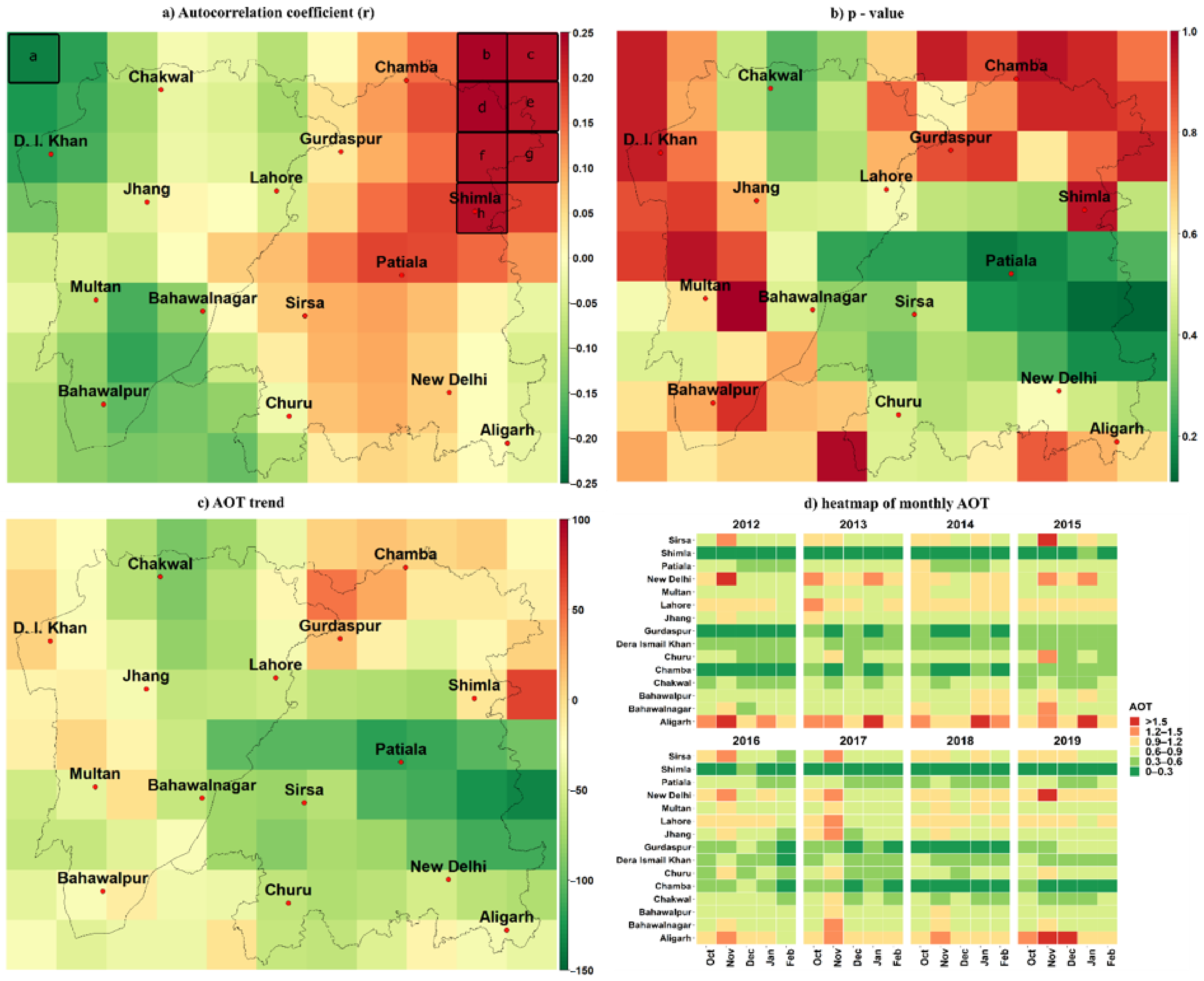
AOT is decreasing in the studied period over Northern and eastern Pakistan with a similarly declining trend of fire events. It is however, increasing in the southern Punjab region.
(2)
This is be due to the strict policy implementation in the north and comparatively lesser attention towards the southern region. As in the north traffic and trade flow is high and usually hampered by low visibility.
(3)
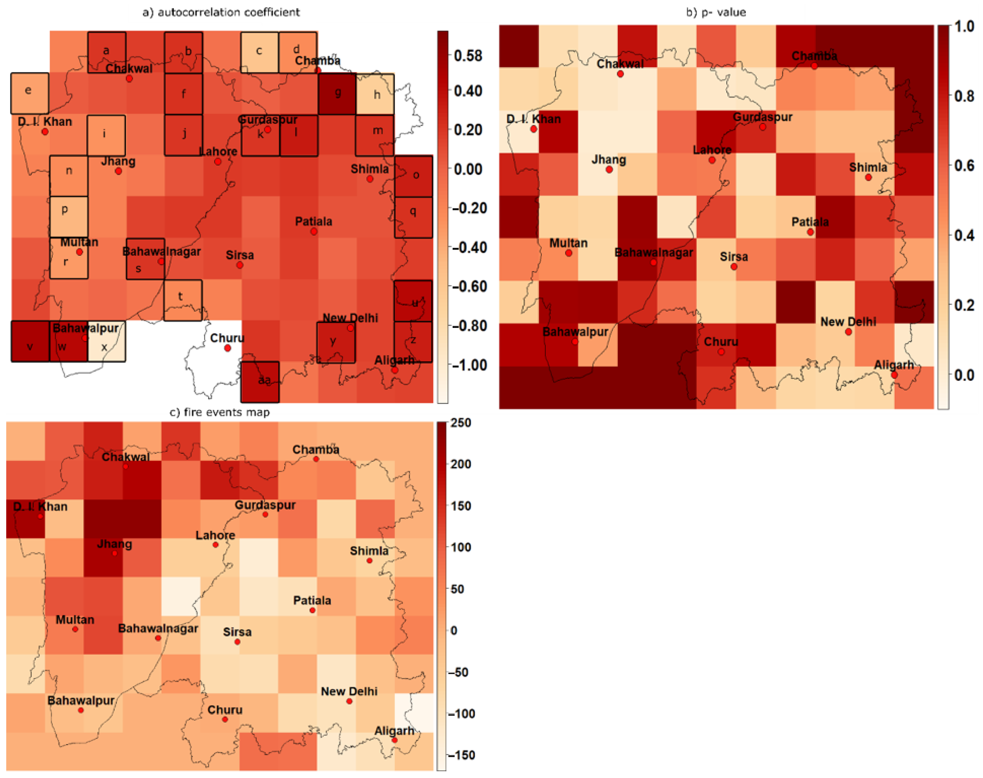
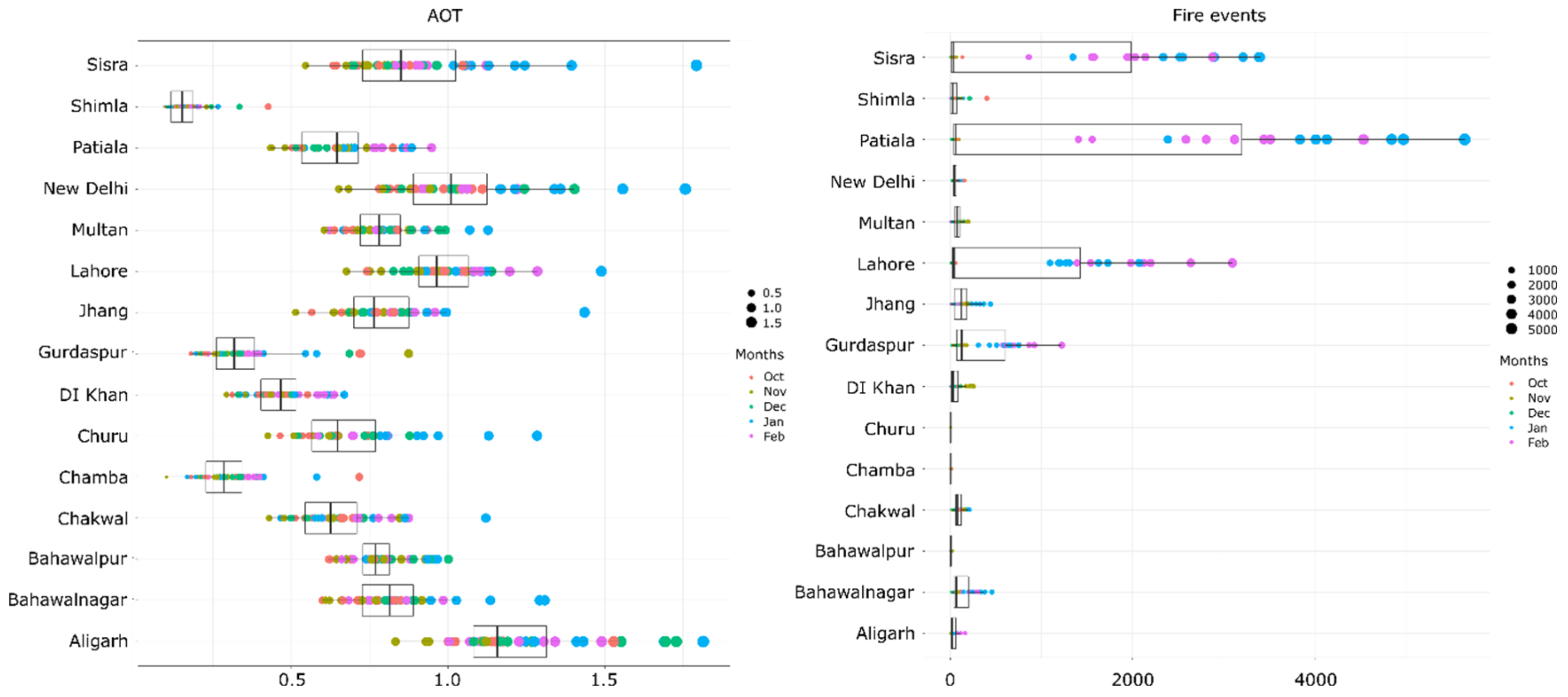
While on the Indian side fire events have substantially increased in the north and central Punjab. And the trend in AOT is high in northern regions. Still Sirsa, Patiala and Lahore led with highest number of fire events from 2012 to 2019 between October and Feb.
(4)
The highest AOT values in the entire study were observed on the Indian side with 26 Indian districts reporting a value above 1.0 followed by Kasur and Lahore In Pakistan at 0.93.
(5)
Similarly, for fire event counts, more than 128,000 events were recorded in Sangrur district followed by another 16 Indian districts then Kasur and Lahore at ~28,000 each.
(6)
For the increasing trend in AOT Yamuna Nagar and Una from India and Vehari from Pakistan topped the list.
(7)
For fire events Sargodha, Khushab, DI Khan and Jhang were notably on the top of the list.
In our future studies we plan to assess this change in trend in the light of crop harvesting and cultivation patterns and relate the high incidences to different crop types and their harvesting period over the studied time.

Author Contributions

Conceptualization, M.U. and S.A.; methodology S.A., A.T., M.A., M.Z.; data processing and manuscript writing, M.U., S.A., M.L.H.; figures and charts, M.U., S.A.; formal validation and analysis of findings, S.A., A.T., M.A., M.Z.; manuscript revisions, M.U., S.A., A.T. All authors have read and agreed to the published version of the manuscript.

Funding

This research received no external funding.

Institutional Review Board Statement

Not applicable.

Informed Consent Statement

Not applicable.

Data Availability Statement

Not applicable.

Conflicts of Interest

The authors declare no conflict of interest.

References

  1. Stocker, T.F.; Qin, D.; Plattner, G.-K.; Tignor, M.; Allen, S.K.; Boschung, J.; Nauels, A.; Xia, Y.; Bex, V.; Midgley, P.M. Climate Change 2013: The Physical Science Basis. Contribution of Working Group I to the Fifth Assessment Report of the Intergovernmental Panel on Climate Change; Cambridge University Press: Cambridge, UK, 2013; p. 1535. [Google Scholar]
  2. Chan, K. Aerosol optical depths and their contributing sources in Taiwan. Atmos. Environ. 2017, 148, 364–375. [Google Scholar] [CrossRef]
  3. Gurjar, B.; Butler, T.; Lawrence, M.; Lelieveld, J. Evaluation of emissions and air quality in megacities. Atmos. Environ. 2008, 42, 1593–1606. [Google Scholar] [CrossRef]
  4. Koren, I.; Altaratz, O.; Remer, L.A.; Feingold, G.; Martins, J.V.; Heiblum, R.H. Aerosol-induced intensification of rain from the tropics to the mid-latitudes. Nat. Geosci. 2012, 5, 118–122. [Google Scholar] [CrossRef]
  5. Koren, I.; Feingold, G. Aerosol-cloud-precipitation system as a predator-prey problem. Proc. Natl. Acad. Sci. USA 2011, 108, 12227–12232. [Google Scholar] [CrossRef] [Green Version]
  6. Pope, C.A., III; Burnett, R.T.; Thun, M.J.; Calle, E.E.; Krewski, D.; Ito, K.; Thurston, G.D. Lung cancer, cardiopulmonary mortality, and long-term exposure to fine particulate air pollution. JAMA 2002, 287, 1132–1141. [Google Scholar] [CrossRef] [PubMed] [Green Version]
  7. Chin, M.; Kahn, R. Atmospheric Aerosol Properties and Climate Impacts; US Climate Change Science Program: Washington, DC, USA, 2009; Volume 2. [Google Scholar]
  8. Kaufman, Y.; Tanré, D.; Remer, L.A.; Vermote, E.; Chu, A.; Holben, B. Operational remote sensing of tropospheric aerosol over land from EOS moderate resolution imaging spectroradiometer. J. Geophys. Res. Atmos. 1997, 102, 17051–17067. [Google Scholar] [CrossRef]
  9. Provençal, S.; Kishcha, P.; da Silva, A.M.; Elhacham, E.; Alpert, P. AOD distributions and trends of major aerosol species over a selection of the world’s most populated cities based on the 1st version of NASA’s MERRA Aerosol Reanalysis. Urban Clim. 2017, 20, 168–191. [Google Scholar] [CrossRef] [PubMed]
  10. Gadde, B.; Bonnet, S.; Menke, C.; Garivait, S. Air pollutant emissions from rice straw open field burning in India, Thailand and the Philippines. Environ. Pollut. 2009, 157, 1554–1558. [Google Scholar] [CrossRef]
  11. Kumar, P.; Kumar, S.; Joshi, L. Socioeconomic and Environmental Implications of Agricultural Residue Burning: A Case Study of Punjab, India; Springer Nature: Berlin, Germany, 2015. [Google Scholar]
  12. Vadrevu, K.P.; Ellicott, E.; Badarinath, K.; Vermote, E. MODIS derived fire characteristics and aerosol optical depth variations during the agricultural residue burning season, north India. Environ. Pollut. 2011, 159, 1560–1569. [Google Scholar] [CrossRef]
  13. Venkataraman, C.; Habib, G.; Kadamba, D.; Shrivastava, M.; Leon, J.F.; Crouzille, B.; Boucher, O.; Streets, D. Emissions from open biomass burning in India: Integrating the inventory approach with high-resolution Moderate Resolution Imaging Spectroradiometer (MODIS) active-fire and land cover data. Glob. Biogeochem. Cycles 2006, 20. [Google Scholar] [CrossRef]
  14. Gultepe, I.; Tardif, R.; Michaelides, S.C.; Cermak, J.; Bott, A.; Bendix, J.; Müller, M.D.; Pagowski, M.; Hansen, B.; Ellrod, G.; et al. Fog Research: A Review of Past Achievements and Future Perspectives. Pure Appl. Geophys. 2007, 164, 1121–1159. [Google Scholar] [CrossRef]
  15. Gultepe, I.; Pagowski, M.; Reid, J. Using surface data to validate a satellite based fog detection scheme. Weather Forecast. 2007, 22, 444–456. [Google Scholar] [CrossRef]
  16. Bulbul, G.; Shahid, I.; Chishtie, F.; Shahid, M.Z.; Hundal, R.A.; Zahra, F.; Shahzad, M.I. PM10 Sampling and AOD Trends during 2016 Winter Fog Season in the Islamabad Region. Aerosol Air Qual. Res. 2018, 18, 188–199. [Google Scholar] [CrossRef] [Green Version]
  17. Shahid, Z.M.; Liao, H.; Li, J.; Shahid, I.; Lodhi, A.; Mansha, M. Seasonal variations of aerosols in Pakistan: Contributions of domestic anthropogenic emissions and transboundary transport. Aerosol Air Qual. Res. 2015, 15, 1580–1600. [Google Scholar] [CrossRef] [Green Version]
  18. Chen, F.; Zhang, X.; Zhu, X.; Zhang, H.; Gao, J.; Hopke, P.K. Chemical Characteristics of PM2.5 during a 2016 Winter Haze Episode in Shijiazhuang, China. Aerosol Air Qual. Res. 2016, 17, 368–380. [Google Scholar] [CrossRef] [Green Version]
  19. Feng, N.; Christopher, S.A. Satellite and surface-based remote sensing of Southeast Asian aerosols and their radiative effects. Atmos. Res. 2013, 122, 544–554. [Google Scholar] [CrossRef]
  20. Griggs, M. Measurements of Atmospheric Aerosol Optical Thickness over Water Using ERTS-1 Data. J. Air Pollut. Control. Assoc. 1975, 25, 622–626. [Google Scholar] [CrossRef] [PubMed] [Green Version]
  21. Kaufman, J.Y.; Tanré, D.; Boucher, O. A satellite view of aerosols in the climate system. Nature 2002, 419, 215–223. [Google Scholar] [CrossRef]
  22. Levy, R.C.; Remer, L.; Kleidman, R.; Mattoo, S.K.; Ichoku, C.; Kahn, R.; Eck, T.F. Global evaluation of the Collection 5 MODIS dark-target aerosol products over land. Atmos. Chem. Phys. Discuss. 2010, 10, 10399–10420. [Google Scholar] [CrossRef] [Green Version]
  23. Levy, C.R.; Remer, L.A.; Dubovik, O. Global aerosol optical properties and application to Moderate Resolution Imaging Spectroradiometer aerosol retrieval over land. J. Geophys. Res. Atmos. 2007, 112. [Google Scholar] [CrossRef] [Green Version]
  24. Remer, A.L.; Kaufman, Y.; Tanré, D.; Mattoo, S.; Chu, D.; Martins, J.V.; Li, R.-R.; Ichoku, C.; Levy, R.; Kleidman, R. The MODIS aerosol algorithm, products, and validation. J. Atmos. Sci. 2005, 62, 947–973. [Google Scholar] [CrossRef] [Green Version]
  25. Boiyo, R.; Kumar, K.R.; Zhao, T.; Bao, Y. Climatological analysis of aerosol optical properties over East Africa observed from space-borne sensors during 2001–2015. Atmos. Environ. 2017, 152, 298–313. [Google Scholar] [CrossRef]
  26. Jackson, M.J.; Liu, H.; Laszlo, I.; Kondragunta, S.; Remer, L.A.; Huang, J.; Huang, H.C. Suomi-NPP VIIRS aerosol algorithms and data products. J. Geophys. Res. Atmos. 2013, 118, 12673–12689. [Google Scholar] [CrossRef]
  27. He, Q.; Li, C.; Tang, X.; Li, H.; Geng, F.; Wu, Y. Validation of MODIS derived aerosol optical depth over the Yangtze River Delta in China. Remote Sens. Environ. 2010, 114, 1649–1661. [Google Scholar] [CrossRef]
  28. Huang, J.; Kondragunta, S.; Laszlo, I.; Liu, H.; Remer, L.A.; Zhang, H.; Superczynski, S.; Ciren, P.; Holben, B.N.; Petrenko, M. Validation and expected error estimation of Suomi-NPP VIIRS aerosol optical thickness and Ångström exponent with AERONET. J. Geophys. Res. Atmos. 2016, 121, 7139–7160. [Google Scholar] [CrossRef] [Green Version]
  29. Meng, F.; Cao, C.; Shao, X. Spatio-temporal variability of Suomi-NPP VIIRS-derived aerosol optical thickness over China in 2013. Remote Sens. Environ. 2015, 163, 61–69. [Google Scholar] [CrossRef]
  30. Kondragunta, S.; Laszlo, I.; Ciren, P.; Zhang, H.; Liu, H.; Huang, J.; Huff, A. Exceptional events monitoring using S-NPP VIIRS aerosol products. In Proceedings of the 2017 IEEE International Geoscience and Remote Sensing Symposium (IGARSS), Fort Worth, TX, USA, 23–28 July 2017; pp. 1285–1287. [Google Scholar] [CrossRef]
  31. Cao, C.; de Luccia, F.J.; Xiong, X.; Wolfe, R.; Weng, F. Early on-orbit performance of the visible infrared imaging ra-diometer suite onboard the Suomi National Polar-Orbiting Partnership (S-NPP) satellite. IEEE Trans. Geosci. Remote Sens. 2013, 52, 1142–1156. [Google Scholar] [CrossRef] [Green Version]
  32. DATA.GOV, VIIRS/SNPP Deep Blue Level 3 Daily Aerosol Data, 1 × 1 Degree Grid. 2020. Available online: https://catalog.data.gov/dataset/viirs-snpp-deep-blue-level-3-daily-aerosol-data-1x1-degree-grid (accessed on 7 December 2020).
  33. Sayer, A.; Hsu, N.; Lee, J.; Bettenhausen, C.; Kim, W.; Smirnov, A. Satellite Ocean Aerosol Retrieval (SOAR) Algorithm Extension to S-NPP VIIRS as Part of the “Deep Blue” Aerosol Project. J. Geophys. Res. Atmos. 2018, 123, 380–400. [Google Scholar] [CrossRef]
  34. Sabetghadam, S.; Khoshsima, M.; Alizadeh-Choobari, O. Spatial and temporal variations of satellite-based aerosol optical depth over Iran in Southwest Asia: Identification of a regional aerosol hot spot. Atmos. Pollut. Res. 2018, 9, 849–856. [Google Scholar] [CrossRef]
  35. Yu, M.; Yuan, X.; He, Q.; Yu, Y.; Cao, K.; Yang, Y.; Zhang, W. Temporal-spatial analysis of crop residue burning in China and its impact on aerosol pollution. Environ. Pollut. 2019, 245, 616–626. [Google Scholar] [CrossRef]
  36. Schroeder, W.; Oliva, P.; Giglio, L.; Csiszar, I.A. The New VIIRS 375m active fire detection data product: Algorithm description and initial assessment. Remote Sens. Environ. 2014, 143, 85–96. [Google Scholar] [CrossRef]
  37. Csiszar, I.; Schroeder, W.; Giglio, L.; Ellicott, E.; Vadrevu, K.P.; Justice, C.O.; Wind, B. Active fires from the Suomi NPP Visible Infrared Imaging Radiometer Suite: Product status and first evaluation results. J. Geophys. Res. Atmos. 2014, 119, 803–816. [Google Scholar] [CrossRef]
  38. Naheed, G.; Kazmi, D.; Rasul, G. Seasonal variation of rainy days in Pakistan. Pak. J. Meteorol. 2013, 9, 9–13. [Google Scholar]
  39. Hartmann, H.; Andresky, L. Flooding in the Indus River basin—A spatiotemporal analysis of precipitation records. Glob. Planet. Chang. 2013, 107, 25–35. [Google Scholar] [CrossRef]
  40. Hartmann, H.; Buchanan, H. Trends in extreme precipitation events in the Indus River Basin and flooding in Pakistan. Atmos. Ocean 2014, 52, 77–91. [Google Scholar] [CrossRef]
  41. Partal, T.; Kahya, E. Trend analysis in Turkish precipitation data. Hydrol. Process. Int. J. 2006, 20, 2011–2026. [Google Scholar] [CrossRef]
  42. Von Storch, H. Misuses of statistical analysis in climate research. In Analysis of Climate Variability; Springer: Berlin/Heidelberg, Germany, 1999; pp. 11–26. [Google Scholar]
  43. Yue, S.; Pilon, P.; Phinney, B.; Cavadias, G. The influence of autocorrelation on the ability to detect trend in hydrological series. Hydrol. Process. 2002, 16, 1807–1829. [Google Scholar] [CrossRef]
  44. Mann, H.B. Nonparametric tests against trend. Econom. J. Econom. Soc. 1945, 13, 245–259. [Google Scholar] [CrossRef]
  45. Jiang, T.; Su, B.; Hartmann, H. Temporal and spatial trends of precipitation and river flow in the Yangtze River Basin, 1961–2000. Geomorphology 2007, 85, 143–154. [Google Scholar] [CrossRef]
  46. Reiter, A.; Weidinger, R.; Mauser, W. Recent Climate Change at the Upper Danube—A temporal and spatial analysis of temperature and precipitation time series. Clim. Chang. 2012, 111, 665–696. [Google Scholar] [CrossRef]
  47. Tabari, H.; Talaee, P.H. Analysis of trends in temperature data in arid and semi-arid regions of Iran. Glob. Planet. Chang. 2011, 79, 1–10. [Google Scholar] [CrossRef]
  48. Wang, Q.-X.; Fan, X.-H.; Qin, Z.-D.; Wang, M.-B. Change trends of temperature and precipitation in the Loess Plateau Region of China, 1961–2010. Glob. Planet. Chang. 2012, 92, 138–147. [Google Scholar] [CrossRef]
  49. Wang, W. Stochasticity, Nonlinearity and Forecasting of Streamflow Processes; IOS Press: Amsterdam, The Netherlands, 2006. [Google Scholar]
  50. Kendall, M. Rank Correlation Methods; Charles Griffin Book Series; Oxford University Press: London, OH, USA, 1975. [Google Scholar]
  51. Hirsch, R.M.; Slack, J.R.; Smith, R.A. Techniques of trend analysis for monthly water quality data. Water Resour. Res. 1982, 18, 107–121. [Google Scholar] [CrossRef] [Green Version]
  52. Khattak, M.; Babel, M.; Sharif, M. Hydro-meteorological trends in the upper Indus River basin in Pakistan. Clim. Res. 2011, 46, 103–119. [Google Scholar] [CrossRef]
  53. Ahmad, I.; Tang, D.; Wang, T.; Wang, M.; Wagan, B. Precipitation Trends over Time Using Mann-Kendall and Spearman’s rho Tests in Swat River Basin, Pakistan. Adv. Meteorol. 2015, 2015, 431860. [Google Scholar] [CrossRef] [Green Version]
  54. Nasri, M.; Modarres, R. Dry spell trend analysis of Isfahan Province, Iran. Int. J. Clim. J. R. Meteorol. Soc. 2009, 29, 1430–1438. [Google Scholar] [CrossRef]
  55. Foster, P.; Ramaswamy, V.; Artaxo, P.; Berntsen, T.; Betts, R.; Fahey, D.; Haywood, J.; Lean, J.; Lowe, D.; Myhre, G. Climate Change 2007: The Physical Science Basis. Intergovernmental Panel on Climate Change; Cambridge University Press: Cambridge, UK; New York, NY, USA, 2007. [Google Scholar]
  56. Syed, F.S.; Körnich, H.; Tjernström, M. On the fog variability over south Asia. Clim. Dyn. 2012, 39, 2993–3005. [Google Scholar] [CrossRef]
  57. Pant, B.G.; Kumar, K.R. Climates of South Asia; Wiley-Blackwell: Hoboken, NJ, USA, 1997. [Google Scholar]
  58. Khan, Z. Air Pollution and Smog. Pakistan Today, 26 November 2019. [Google Scholar]
  59. Alam, K.; Trautmann, T.; Blaschke, T.; Majid, H. Aerosol optical and radiative properties during summer and winter seasons over Lahore and Karachi. Atmos. Environ. 2012, 50, 234–245. [Google Scholar] [CrossRef]
  60. Biswas, S.; Hu, S.; Verma, V.; Herner, J.D.; Robertson, W.H.; Ayala, A.; Sioutas, C. Physical properties of particulate matter (PM) from late model heavy-duty diesel vehicles operating with advanced PM and NOx emission control technologies. Atmos. Environ. 2008, 42, 5622–5634. [Google Scholar] [CrossRef]
  61. Badarinath, K.; Kharol, S.K.; Sharma, A.R.; Prasad, V.K. Analysis of aerosol and carbon monoxide characteristics over Arabian Sea during crop residue burning period in the Indo-Gangetic Plains using multi-satellite remote sensing datasets. J. Atmos. Solar Terr. Phys. 2009, 71, 1267–1276. [Google Scholar] [CrossRef]
  62. Hussain, A.; Mir, H.; Afzal, M. Analysis of dust storms frequecny over pakistan during 1961–2000. Pak. J. Meteorol. 2005, 2, 49–68. [Google Scholar]
  63. Sharma, R.A.; Kharol, S.K.; Badarinath, K.; Singh, D. Impact of agriculture crop residue burning on atmospheric aerosol loading—A study over Punjab State, India. Ann. Geophys. 2010, 28, 09927689. [Google Scholar]
  64. Tariq, S.; Ali, M. Spatio–temporal distribution of absorbing aerosols over Pakistan retrieved from OMI onboard Aura satellite. Atmos. Pollut. Res. 2015, 6, 254–266. [Google Scholar] [CrossRef] [Green Version]
  65. Yasmeen, Z.; Rasul, G.; Zahid, M. Impact of aerosols on winter fog of Pakistan. Pak. J. Meteorol. 2012, 8, 21–30. [Google Scholar]
  66. Khokhar, M.F.; Yasmin, N.; Chishtie, F.; Shahid, I. Temporal Variability and Characterization of Aerosols across the Pakistan Region during the Winter Fog Periods. Atmosphere 2016, 7, 67. [Google Scholar] [CrossRef] [Green Version]
  67. Popovich, N.B.M.; Patanjali, K.; Singhvi, A.; Huang, J. See How the World’s Most Polluted Air Compares with Your City’s. 2019. Available online: https://www.nytimes.com/interactive/2019/12/02/climate/air-pollution-compare-ar-ul.html (accessed on 12 January 2020).
  68. Shabbir, M.; Junaid, A.; Zahid, J. Smog: A Transboundary Issue and Its Implications in India and Pakistan; Sustainable Development Policy Institute: Islamabad, Pakistan, 2019. [Google Scholar]
  69. Raza, W.; Saeed, S.; Saulat, H.; Gul, H.; Sarfraz, M.; Sonne, C.; Sohn, Z.-H.; Brown, R.J.; Kim, K.-H. A review on the deteriorating situation of smog and its preventive measures in Pakistan. J. Clean. Prod. 2020, 279, 123676. [Google Scholar] [CrossRef]
  70. Alam, K.; Qureshi, S.; Blaschke, T. Monitoring spatio-temporal aerosol patterns over Pakistan based on MODIS, TOMS and MISR satellite data and a HYSPLIT model. Atmos. Environ. 2011, 45, 4641–4651. [Google Scholar] [CrossRef]
  71. El-Askary, H.; Gautam, R.; Singh, R.; Kafatos, M. Dust storms detection over the Indo-Gangetic basin using multi sensor data. Adv. Space Res. 2006, 37, 728–733. [Google Scholar] [CrossRef]
  72. Kant, S.; Panda, J.; Gautam, R. A seasonal analysis of aerosol-cloud-radiation interaction over Indian region during 2000–2017. Atmos. Environ. 2019, 201, 212–222. [Google Scholar] [CrossRef]
  73. Kaskaoutis, D.; Sinha, P.; Vinoj, V.; Kosmopoulos, P.; Tripathi, S.; Misra, A.; Sharma, M.C.; Singh, R. Aerosol properties and radiative forcing over Kanpur during severe aerosol loading conditions. Atmos. Environ. 2013, 79, 7–19. [Google Scholar] [CrossRef]
  74. Liu, T.; Mickley, L.J.; Gautam, R.; Singh, M.K.; DeFries, R.S.; Marlier, M. Detection of delay in post-monsoon agricultural burning across Punjab, India: Potential drivers and consequences for air quality. Environ. Res. Lett. 2020, 16, 014014. [Google Scholar] [CrossRef]
  75. Imam, A.U.K.; Banerjee, U.K. Urbanisation and greening of Indian cities: Problems, practices, and policies. Ambio 2016, 45, 442–457. [Google Scholar] [CrossRef] [Green Version]
  76. Ningombam, S.S.; Dumka, U.C.; Srivastava, A.; Song, H.-J. Optical and physical properties of aerosols during active fire events occurring in the Indo-Gangetic Plains: Implications for aerosol radiative forcing. Atmos. Environ. 2020, 223, 117225. [Google Scholar] [CrossRef]
  77. Sharma, D.; Singh, D.; Kaskaoutis, D.G. Impact of Two Intense Dust Storms on Aerosol Characteristics and Radiative Forcing over Patiala, Northwestern India. Adv. Meteorol. 2012, 2012, 1–13. [Google Scholar] [CrossRef] [Green Version]
  78. Mishra, A.; Srivastava, A.; Jain, V. Spectral dependency of aerosol optical depth and derived aerosol size distribution over Delhi: An implication to pollution source. Sustain. Environ. Res. 2013, 23, 113–128. [Google Scholar]
  79. Kumar, P.; Mann, M.; Gupta, N.C. Regression analysis of aerosol optical properties with long-term MODIS data using forward selection method. Meteorol. Atmos. Phys. 2019, 131, 1121–1131. [Google Scholar] [CrossRef]
  80. Lodhi, N.K.; Beegum, S.N.; Singh, S.; Kumar, K. Aerosol climatology at Delhi in the western Indo-Gangetic Plain: Microphysics, long-term trends, and source strengths. J. Geophys. Res. Atmos. 2013, 118, 1361–1375. [Google Scholar] [CrossRef]
  81. Saha, D.; Soni, K.; Mohanan, M.; Singh, M. Long-term trend of ventilation coefficient over Delhi and its potential impacts on air quality. Remote Sens. Appl. Soc. Environ. 2019, 15, 100234. [Google Scholar] [CrossRef]
  82. Soni, K.; Kapoor, S.; Parmar, K.S.; Kaskaoutis, D.G. Statistical analysis of aerosols over the Gangetic-Himalayan region using ARIMA model based on long-term MODIS observations. Atmos. Res. 2014, 149, 174–192. [Google Scholar] [CrossRef]
  83. Kutty, S.G.; Dimri, A.P.; Gultepe, I. Climatic trends in fog occurrence over the Indo-Gangetic plains. Int. J. Clim. 2020, 40, 2048–2061. [Google Scholar] [CrossRef]
Figure 1. The ‘Study Area’ consists of the northeastern region of Pakistan (31 districts Punjab, along with one district from Khyber Pakhtunkhwa and Azad Jammu and Kashmir) and India (two provinces Haryana, Punjab, twenty divisions from Himachal Pradesh, Uttaranchal, Uttar Pradesh, Rajasthan, and New Delhi (capital)).
Atmosphere 12 00242 g001
Figure 2. (a) Autocorrelation coefficient (r) for AOT is displayed in which high values are depicted by red color and green color is for the low values. Highlighted timeseries (a–h) were found significantly autocorrelated (exceeds the range of value 0.2) and thus replaced by pre-whitening time Scheme 0. 0). Time series those have value of 0.2 were considered to have significant trend. (b) p-values were high for the northwestern region of Punjab in Pakistan and Northern India. (c) Mann-Kendall Score for AOT displays the increasing (red color) or decreasing (green color) trend. It was found that Kendall score for AOT have a significantly increasing trend towards the Pakistani region. (d) Heatmaps of the relative distribution of monthly mean of AOT among winter season; each month is identified by separate color over fifteen selected cities in the study area.
Atmosphere 12 00242 g002
Figure 3. (a) Autocorrelation coefficient (r) map for ’Fire Events’ displaying high values of by red color and low values by green color. Time series those exceeds the range of value 0.2 was considered as autocorrelated time series as highlighted (a) and these autocorrelated timeseries were replaced by pre-whitening timeseries. (b) p-value for ’Fire Events’ map high values are displayed by red color and low values by green color. Time sires those values does not exceeds 0.2 were considered to have a significant trend. (c) Mann-Kendall Score for ’Fire Events’ displayed the increasing (red color) or decreasing (green color) trend. It was recorded that Kendall score for ’Fire Events’ have a the significantly increasing trend towards the Pakistani region.
Atmosphere 12 00242 g003
Figure 4. Scatterplots of monthly values of AOT and fire events in the selected administrative regions of Indian and Pakistani. High number of fire counts were recorded during the months of October and November.
Atmosphere 12 00242 g004
Figure 5. (a) A step wise analysis of NDVI loss to harvesting and (b) its correlation with fire events in the study area. The top (b1) and bottom heatmaps (b2) represents the annual district wise recorded AOT in the study area for Punjab in Pakistan and Punjab in India, respectively. Districts have been arranged from east to west.
Atmosphere 12 00242 g005
Figure 6. Seasonal and overall prevailing wind direction in the study area. The winter months and the overall direction suggests that the winds are primary carriers of pollutants from Punjab in India Over to the Pakistani side.
Atmosphere 12 00242 g006
Table 1. Datasets used in this study with their features.
ProductSpatial ResolutionTemporal Resolution UsedData Acquisition Dates
Aerosol Optical Depth (AOD)1° × 1°1 day1 October 2012–28 February 2020
Fire Hotspot375 × 375 m3 h (converted to daily)1 October 2012–28 February 2020
Table 2. Number of times series pre-whitened with respect to different datasets.
Sr. NoVariable NameTotal no. Of Pixel (Time Series)No. Of Pixel Pre-Whitened
1AOT998
2Fire Events8428
Table 3. Autocorrelation coefficients r 1 and the results of Mann-Kendall trend test for AOT over all cities around the study area.
NationCity r 1 p-ValueKendall Score (S) Z M K
IndiaAligarh0.0030.717−31−0.801
Chamba0.0960.866150.374
Churu−0.0190.468−61−1.603
Gurdaspur0.0340.866150.374
New Delhi0.0660.545−51−1.336
Patiala0.1820.153−119−3.153
Shimla0.231 *0.961−5−0.107
Sirsa0.0660.345−79−2.084
PakistanBahawalnagar−0.1180.483−59−1.55
Bahawalpur−0.1190.735−29−0.748
Chakwal−0.0290.287−89−2.351
Dera Ismail Khan−0.1870.94270.16
Jhang−0.040.717−31−0.801
Lahore−0.0480.529−53−1.389
Multan−0.0730.628−41−1.069
* Significant at the 5% level; other statistics based on pre-whitened series.
Table 4. Autocorrelation coefficients r 1 and the results of Mann-Kendall trend test for ‘Fire Events‘ over all cities around the study area.
NationCity r 1 p-ValueKendall Score (S) Z M K
IndiaAligarh0.1110.15−98−0.902
Chamba−0.237 *0.88490.074
Churu00.77230.019
Gurdaspur0.202 *0.753270.242
New Delhi0.335 *0.226−101−0.93
Patiala0.1680.255−95−0.874
Shimla0.070.306−67−0.614
Sirsa0.1230.232−96−0.883
PakistanBahawalnagar0.203 *0.92390.074
Bahawalpur0.429 *0.863−15−0.13
Chakwal0.0980.0181961.813
Dera Ismail Khan−0.229 *0.0112111.952
Jhang−0.1740.0132061.906
Lahore0.1710.506−56−0.511
Multan−0.307 *0.453630.576
* Significant at the 5% level; other statistics based on pre-whitened series.
Publisher’s Note: MDPI stays neutral with regard to jurisdictional claims in published maps and institutional affiliations.

