Modifications to Snow-Melting and Flooding Processes in the Hydrological Model—A Case Study in Issyk-Kul, Kyrgyzstan

Abstract

Streamflow impacts water supply and flood protection. Snowmelt floods occur frequently, especially in mountainous areas, and they pose serious threats to natural and socioeconomic systems. The current forecasting method relies on basic snowmelt accumulation and has geographic limitations that restrict the accuracy and timeliness of flood simulation and prediction. In this study, we clarified the precipitation types in two selected catchments by verifying accumulated and maximum temperatures’ influences on snow melting using a separation algorithm of rain and snow that incorporates with the temperatures. The new snow-melting process utilizing the algorithm in the soil and water assessment tool model (SWAT) was also developed by considering the temperatures. The SWAT model was used to simulate flooding and snowmelt in the catchments. We found that the contributions of snowmelt to the river flow were approximately 6% and 7% higher, according to our model compared to the original model, for catchments A and B, respectively. After the model improvement, the flood peaks increased by 49.42% and 43.87% in A and B, respectively. The contributions of snowmelt to stream flow increased by 24.26% and 31% for A and B, respectively. Generally, the modifications improved the model accuracy, the accuracy of snowmelt’s contributions to runoff, the accuracy of predicting flood peaks, the time precision, and the flood frequency simulations.

1. Introduction

Water resources are essential for society’s long-term development, economic growth, and ecological environment [1,2,3,4]. Large amounts of water are stored as snow and glaciers [5,6], and this water can be discharged into catchments [7,8,9]. Approximately one-sixth of the world’s population lives near rivers that originate from snowmelt [10], which can occur in mountainous areas, even in otherwise arid regions. The melt water is used for agricultural, industrial, and municipal purposes [11]; however, its availability may alternate the water levels of lakes and cause floods that can pose serious threats to natural and socioeconomic systems. According to recent statistics, mountain torrents were responsible for approximately 70% of flood-related deaths [12,13], and associated disaster losses accounted for more than 50% of the total deaths [14,15]. Frequent floods may pose a significant threat to certain populations, especially those in high-altitude areas, such as Kyrgyzstan. Indeed, Kyrgyzstan is among the countries affected by such floods.

Kyrgyzstan is a Central Asian country with abundant underground and surface water resources. Changes in the runoff and distribution of its sources, mainly rainfall, snowmelt water, glaciers, and other tributaries, affect the water in Issyk-Kul, Kyrgyzstan’s large endorheic lake [16]. The Issyk-Kul basin contains a number of streams. About 123 of them are used for irrigation [17,18]. Water supply and flood protection are both impacted by streamflow [19,20]. Furthermore, Issyk-Kul is fed by rivers, the majority of whose water comes from snow and glaciers, which cover about 509 km² of the drainage basin and are located at elevations of 3000 m a.s.l. and higher [21,22,23]. Precipitation increases from May to August, corresponding with a seasonal increase in agricultural water demand [16]. During the summer (June to September), rivers primarily fed by glacial meltwater experience significant increases in runoff, resulting in floods during the “flood season” [5]. There are four types of rivers. The majority of glacial-snow-type rivers flow into Issyk-Kul [24]. River runoff’s shifting properties have long been focuses of hydrological and water resource research [25]. Since Issyk-Kul’s rivers affect its water level, it is important to focus on the sources of the rivers, especially the snowmelt.

Snowmelt runoff is a significant source of water and a substantial driving force for catastrophic flooding in inland desert regions during the spring flood season, so it must be carefully analyzed. To mitigate or minimize the tragedies and losses caused by floods, it is vital to analyze the complete snow melting and flood process [26]. Many models have been developed, including empirical models, conceptual models, physical models, and distributed hydrological models with snowmelt modules [27,28,29,30,31,32,33]. Water balance is calculated by analyzing evaporation during strong winds, low relative humidity, and low temperatures [34]. More advanced models [35,36] were shown to be flawed when simulating runoff in snowmelt watersheds [37]. The soil water assessment tool (SWAT) [38,39,40] is a distributed watershed hydrological model developed by the US Department of Agriculture and relies on the Simulator for Water Resources in Rural Basins (SWRRB) model [41,42,43,44]. It has good precision when dealing with plains with abundant precipitation and flat terrain, but it has relatively lower accuracy when dealing with mountainous areas with complex terrains [37,45]. The model uses few parameters and little input data. For snow watersheds, the model is used to evaluate dispersed snowmelt and runoff formation [46]. The degree-day factor approach is used in the SWAT model to calculate snowmelt [35,47,48]. In this approach, snowmelt is considered to occur when the average temperature on a given day exceeds the snow-melting temperature threshold. However, the condition for snowmelt is only the daily average temperature, thereby ignoring the influence of cumulative temperature on energy accumulation [49]. Previous researchers, such as Meng et al., Yu et al., and Luo et al., attempted to use the SWAT model with the snowmelt module, but there was confusion about how to distinguish precipitation types. Other studies failed to account for the conditions of mountainous regions, expended immense amounts of effort, or relied on the standard degree-day factor system (which provides limited simulation accuracy) [36,37,50]. Improvements to precipitation type recognition have been ignored in related attempts to enhance snow-related models which omit the standard degree-day factor technique. Therefore, based on recent analysis, the determination of precipitation type was used in this study, and the classic degree-day factor approach was updated. The goal of this research was to differentiate rain from snow in total precipitation by adding accumulated temperature to the temperature condition. Thereby, the accuracy of the original model was improved to raise its ability to determine precipitation type. The temperature condition of the traditional degree-day factor method was improved by adding an accumulated temperature judgment condition and modifying the parameter set. This improved the simulation accuracy of the model [9,37] and improved the calculations of snowmelt capacity and snowmelt’s contributions to runoff in the selected catchments around Issyk-Kul.

2. Study Area and Materials

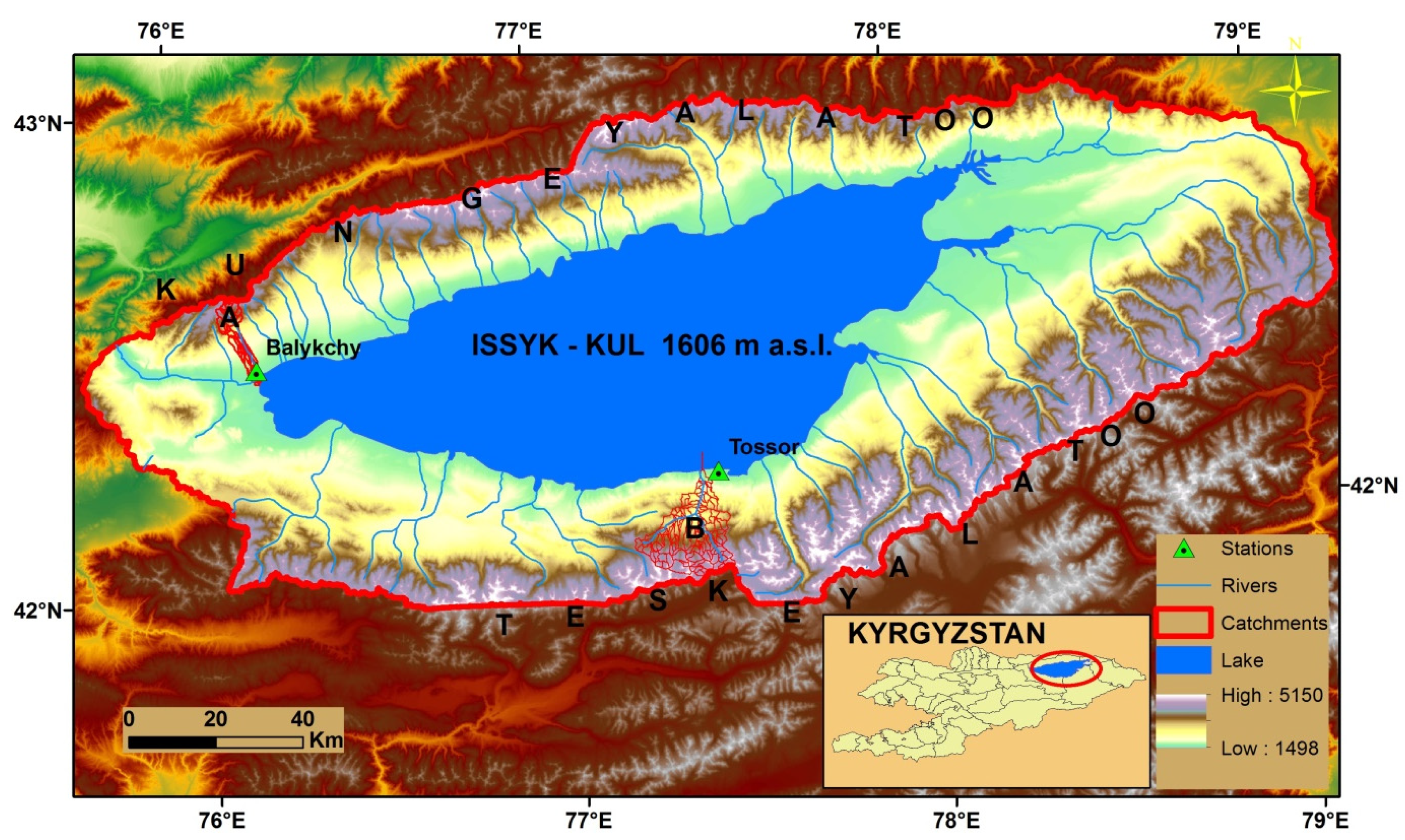
2.1. Study Area

The Issyk-Kul basin is located on the northern slopes of the Tian-Shan Mountains in Kyrgyzstan, which is part of arid Central Asia, between 42°250 N and 77°150 E (Figure 1), at an altitude of 1606 m above sea level (a.s.l.) [51]. Issyk-Kul is the continent’s fourth-deepest reservoir. It is an endogenous mountain lake (one of the world’s highest saline lakes). It is Central Asia’s largest high-altitude lake [52]. It is surrounded by high mountains, such as Teskey Ala-Too, a mountain range to the south with peaks exceeding 4808 m, and Kungey Ala-Too, a mountain range to the north with peaks exceeding 4648 m. Its watershed covers an area of 22,080 km², and all major branches of Issyk-Kul originate from 834 g1aciers with a volume of 48 km³ and a total glacial area of 650 km² [53,54].

One of Kyrgyzstan’s most densely populated areas is around Issyk-Kul. With an average annual growth rate of 1.84%, the population of its Oblast increased from 177,300 in 1940 to 448,000 in 2012 [55]. The moderately warm climate of the Issyk-Kul basin is ideal for cereals, crops, and gardening [16,56]. The average temperature in the basin is 19–20 °C in July and 2–3 °C in January, and precipitation ranges from 12.3–35 mm per year [16]. Intensive agriculture has developed throughout the lake basin due to the basin’s unusually mild climate [57,58,59]. Therefore, we selected two catchments in the Issyk-Kul basin, one in the northwest (A) and the other in the south (B), with areas of 2153.46 km² and 2254.32 km², respectively. The aim of this study was to improve the modelling processes of the selected catchments by incorporating accumulated temperature, allowing for better differentiation of rain and snow in overall precipitation.

2.2. Data and Source

The hydrological model (SWAT) was built with the help of digital elevation models (DEMs), land cover, soil classification, meteorological data, and precipitation type event statistics. A DEM with a resolution of 30 m was downloaded from the Shuttle Radar Topography Mission (SRTM); (http://srtm.csi.cgiar.org/ (accessed on 22 January 2020)). The visual interpretation of the Landsat 8 with 30-meter resolution remote sensing imagery extracted from (https://www.usgs.gov/products/data-and-tools/real-time-data/remote-land-sensing-and-landsat (accessed on 30 December 2019)) provided land use data. The Food and Agriculture Organization (FAO) and the International Institute for Applied Systems Analysis (IIASA) provided the soil data, which included a 1:100,000 soil type map and information on related soil properties. Local Meteorological stations provided precipitation type event statistics. The stations Balykchy and Tossor also provided daily maximum and minimum temperature data (MAX.T and MIN.T, respectively), along with average daily temperatures and precipitation data. The altitude, solar radiation, relative humidity, wind speed, and wind direction data of catchments A and B were collected from the Meteorological Service of Canada (MSC) https://www.canada.ca/en/environment-climate-change/services/climate-change/canadian-centre-climate-services/display-download.html (accessed on 3 February 2020). Model input data (snow cover) were provided by the MODIS snow product MODA10A2.006, with data for 500 m, 8-day, and from 2015 to 2016. We used the data to determine the corresponding temperature thresholds. The Kyrgyzstan hydrological bureau provided daily discharge data from 2015 to 2016, which were used to validate the model.

3. Methods

The daily accumulated temperature was calculated using the temperature integral method. The accumulated temperature inflection points of the precipitation type and snow melting were validated by remote sensing snow data. The traditional degree-day factor, precipitation type determination, and accumulated and maximum temperatures for snow melting were used in this study.

3.1. SWAT Model Definition

The SWAT model is a hydrological, physically-based, and distributed model [60,61]. It uses the runoff curve number approach from the soil conservation service (SCS) to quantify surface runoff and the degree-day factor method to measure snowmelt runoff. The model simulates snowmelt runoff, surface runoff [39,62,63]. The average runoff for the whole watershed is calculated using the hydrological model [37,64]. The water balance equation for the SWAT model is the following:

$${\mathrm{sw}}_{\mathrm{t}}={\mathrm{sw}}_0+{\mathsf{\Sigma }}_{\mathrm{n}=1}^{\mathrm{t}}\left(Nday-Qsurf-Ea-Rseep-Qgw\right)$$

(1)

The final soil water content is denoted by ${\mathrm{sw}}_{\mathrm{t}}$ (mm H₂O), ${\mathrm{sw}}_0$ is the soil water content on day $\mathrm{i}$ (mm H₂O), $\mathrm{t}$ is the time (days), N$day$ is the amount of precipitation on day $\mathrm{n}$ (mm H₂O), $Qsurf$ is the amount of surface runoff on day$\mathrm{n}$ (mm H₂O), the initial soil water content is ${\mathrm{sw}}_0$,$Ea$ is the quantity of evapotranspiration on day $\mathrm{n}$ (mm H₂O), $Rseep$ is the amount of water from the soil profile that enters the vadose region on day$\mathrm{n}$ (mm H₂O), and $Qgw$ is the groundwater recharge (water that is not consumed by evapotranspiration) on day$\mathrm{n}$(mm H₂O).

3.2. Snow Cover in the SWAT Model

The mean daily air temperature is used in the SWAT model to classify precipitation as rain or freezing rain/snow. The boundary temperature,$k_{s-r}$, is set by the user and is used to classify precipitation as rain or snow. The mass balance of the snow pack is as follows:

$$SN{O}_i=SN{O}_{i-1}+R_{da{y}_i}-E_{su{b}_i}-SN{O}_{ml{t}_i}$$

(2)

where $SN{O}_i$ and $SN{O}_{i-1}$ are the water content of the snow pack on the current day ($i$) and previous day ($i-1$), respectively (mm H₂O), $R_{da{y}_i}$ is the amount of precipitation on a given day (added only if ${\overline{\mathrm{k}}}_{\mathrm{av}}\le \mathrm{k}$ (mm H₂O)), $E_{su{b}_i}$ is the amount of sublimation on a given day (mm H₂O), and $SN{O}_{ml{t}_i}$ is the amount of snowmelt on a given day (mm H₂O). The equation for the areal depletion curve is

$$SN{O}_{cov}=\frac{SNO}{SN{O}_{100}}\cdot {\left(\frac{SNO}{SN{O}_{100}}+\exp \left(co{v}_1-co{v}_2\cdot \frac{SNO}{SN{O}_{100}}\right)\right)}^{-1}$$

(3)

where $SN{O}_{cov}$ is the fraction of the HRU area covered by snow, $SNO$ is the water content of the snow pack on the current day (mm H₂O), $SN{O}_{100}$ is the threshold depth of snow at 100% coverage (mm H₂O), and$co{v}_1$ and $co{v}_2$ are coefficients that define the shape of the curve.

3.3. The Original Degree-Day Factor Algorithm

The snowmelt in the SWAT model is important, as is the source of water during the alpine spring [65,66]. The snowmelt runoff temperature threshold is obtained from the snow cover state and the temperature threshold of the snowmelt runoff [67]. The melting snow equation is given below.

$${SNO}_{mlt}={\mathrm{y}}_{mlt}\cdot Sn{o}_{\mathrm{cov}}\cdot \left[\frac{{\mathrm{K}}_{\mathrm{snow}}+{\mathrm{K}}_{\mathrm{mx}}}{2}-{\mathrm{K}}_{mlt}\right]$$

(4)

The total snowmelt on a given day (mm H₂O) is represented by ${SNO}_{mlt}$. ${\mathrm{y}}_{mlt}$ stands for the day’s melt factor (mm H₂O/°C day⁻¹). The fraction of the HRU region is represented by$Sn{o}_{\mathrm{cov}}$. ${\mathrm{K}}_{\mathrm{snow}}$ represents the temperature of the snow pack. ${\mathrm{K}}_{\mathrm{mx}}$ is the highest air temperature on a given day (°C), and ${\mathrm{K}}_{mlt}$ is the base temperature threshold (°C) for snow being able to melt. On a daily basis, the classical degree-day model links ice or snowmelt (mm) to air temperature [68]:

$$\mathrm{M}=\{\begin{array}{ll}r\cdot \left({\mathrm{K}}_{\mathrm{av}}-{\mathrm{K}}_{\mathrm{gmlt}}\right), & \mathrm{when} {\mathrm{K}}_{\mathrm{av}}>{\mathrm{K}}_{\mathrm{gmlt}}\\ 0, & \mathrm{otherwise}\end{array}$$

(5)

where $\mathrm{M}$ is the melt rate, r (mm day⁻¹ °C) is the degree-day factor for snowmelt, ${\mathrm{K}}_{\mathrm{av}}$ (°C) is the average air temperature of a given day, and ${\mathrm{K}}_{\mathrm{gmlt}}$ is the snowmelt base temperature in °C. The degree-day factor for snowmelt is calculated in the SWAT model with a sinusoidal function to simulate the seasonal shift pattern [69]. The temperature of the snow pack is:

$${\mathrm{K}}_{\mathrm{snowp}}={\mathrm{K}}_{{\mathrm{snow}}_{\mathrm{p}-1}}\cdot \left(1-{\mathsf{\alpha }}_{\mathrm{sno}}\right)+{\mathrm{K}}_{\mathrm{av}}\cdot {\mathsf{\alpha }}_{\mathrm{sno}}$$

(6)

${\mathrm{K}}_{\mathrm{snowp}}$ is the temperature (°C) of the snow pack on a given day. ${\mathsf{\alpha }}_{\mathrm{sno}}$ is the snow temperature (°C), which takes into account the previous day’s snow pack temperature. ${\mathrm{K}}_{\mathrm{av}}$ is the average air temperature (°C) on the current day. ${\mathsf{\alpha }}_{\mathrm{sno}}$ is used to represent the influence of linkages among factors affecting snow pack temperature. ${\mathrm{y}}_{mlt}$ is the melt factor, which incorporates the seasonal alterations in maximum and minimum temperature values that happen during dry and wet periods, respectively. The snow/ice melt factor is calculated using sinusoidal interpolation in some snow/ice melt–runoff models [70]. The degree-day factor for snowmelt is expressed as follows:

$${\mathrm{y}}_{mlt}=\frac{{\mathrm{y}}_{mlt6}+{\mathrm{y}}_{mlt12}}{2}+\frac{{\mathrm{y}}_{mlt6}-{\mathrm{y}}_{mlt12}}{2}\cdot \sin \left(\frac{2\mathsf{\pi }}{365}\cdot \left(p-81\right)\right)$$

(7)

where ${\mathrm{y}}_{mlt6}$(mm H₂O day⁻¹ °C⁻¹) is the melt factor for 21 June, ${\mathrm{y}}_{mlt12}$ (mm H₂O day⁻¹ °C⁻¹) is the melt factor for 21 December, and$p$ denotes the number of days in a year. The model divides any sub-basin into several elevation zones [71].

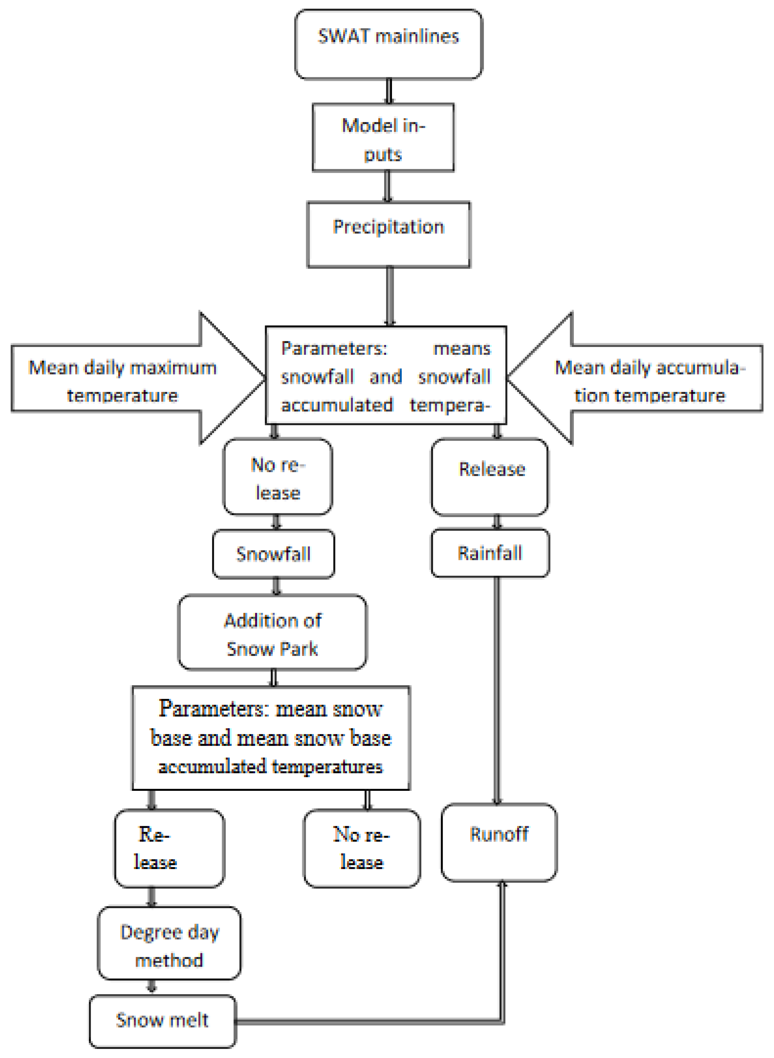
3.4. Model Modifications: Accumulated Temperature and Differentiation of Snowfall and Rainfall

Previous studies, such as [66,67,68,69], revealed that the accumulated temperature can only affect the form of precipitation and the determination of snow melting when the minimum air temperature is above 0 °C. The melt factor is calculated using the following equation:

$$\mathrm{T}=\left({\mathrm{T}}_{max}-{\mathrm{T}}_{min}\right)\sin \mathrm{t}+{\mathrm{T}}_{min}0\le \mathrm{t}\le \mathsf{\pi }$$

(8)

T denotes the temperature at any given time of day; ${\mathrm{T}}_{max}$ and ${\mathrm{T}}_{min}$ are the highest and lowest temperatures ever recorded in a single day, respectively; and t is the value of the arc in a single moment. The equation used to calculate the accumulated temperature when the maximum daily air temperature is greater than 0 °C and the minimum daily air temperature is less than 0 °C is as follows:

$$\mathrm{T}=\{\begin{array}{c}{{\displaystyle \int }}_0^{\pi }\left({\mathrm{T}}_{max}-{\mathrm{T}}_{min}\right)\sin \mathrm{t}+{\mathrm{T}}_{min}du,u\in \left(0,\pi \right)\\ {{\displaystyle \int }}_{{\sin }^{-1}\left(\frac{-{\mathrm{T}}_{min}}{{\mathrm{T}}_{max}-{\mathrm{T}}_{min}}\right)}^{\pi -{\sin }^{-1}\left(\frac{-{\mathrm{T}}_{min}}{{\mathrm{T}}_{max}-{\mathrm{T}}_{min}}\right)}{\mathrm{T}}_{max}\sin \mathrm{udu},\mathrm{u}\in \left( {\sin }^{-1}\left(\frac{-{\mathrm{T}}_{min}}{{\mathrm{T}}_{max}-{\mathrm{T}}_{min}}\right)\right),\pi - {\sin }^{-1}\left(\frac{-{\mathrm{T}}_{min}}{{\mathrm{T}}_{max}-{\mathrm{T}}_{min}}\right)\end{array}$$

(9)

The${\sin }^{-1}\left(\frac{-{\mathrm{T}}_{min}}{{\mathrm{T}}_{max}-{\mathrm{T}}_{min}}\right)$ $\mathrm{and}\pi -{\sin }^{-1}\left(\frac{-{\mathrm{T}}_{min}}{{\mathrm{T}}_{max}-{\mathrm{T}}_{min}}\right)$ represent Radian values when the temperature is 0 °C. The determination of precipitation type and snowmelt calculations are primarily based on the maximum temperature on a given day, the average temperature on that same day, and the set threshold value, while neglecting the accumulated temperature as an important factor affecting both the precipitation type and the snowmelt process [72,73].

Our modified method of snow melting is mentioned in segments (for the original model, see Figure 2). The modifications were added to distinguish between snow and rain. The modified model requires spatial and weather data, and the types of precipitation are determined by applying accumulated and maximum temperatures to HRUs. If the temperature requirement for rainfall is reached, the precipitation is classed as rainfall, and the contribution of rainfall to river flow is estimated using processes from the original model. Snow can melt when accumulated and maximum temperatures fulfill the prescribed conditions at the same time. The snow pack is formed when there is no release of snowfall and snowfall accumulates. If the type of precipitation is found to be snowfall, snowfall is added to the snow pack. When snow-melting conditions are satisfied, the amount of snow melting and its contribution to river runoff are both measured at the same time; otherwise, there is no snowmelt. In other words, the degree-day factor has been corrected, as snowmelt conditions are calculated by adding accumulated and maximum temperatures, and the model was also improved by making it ignore non-melt periods.

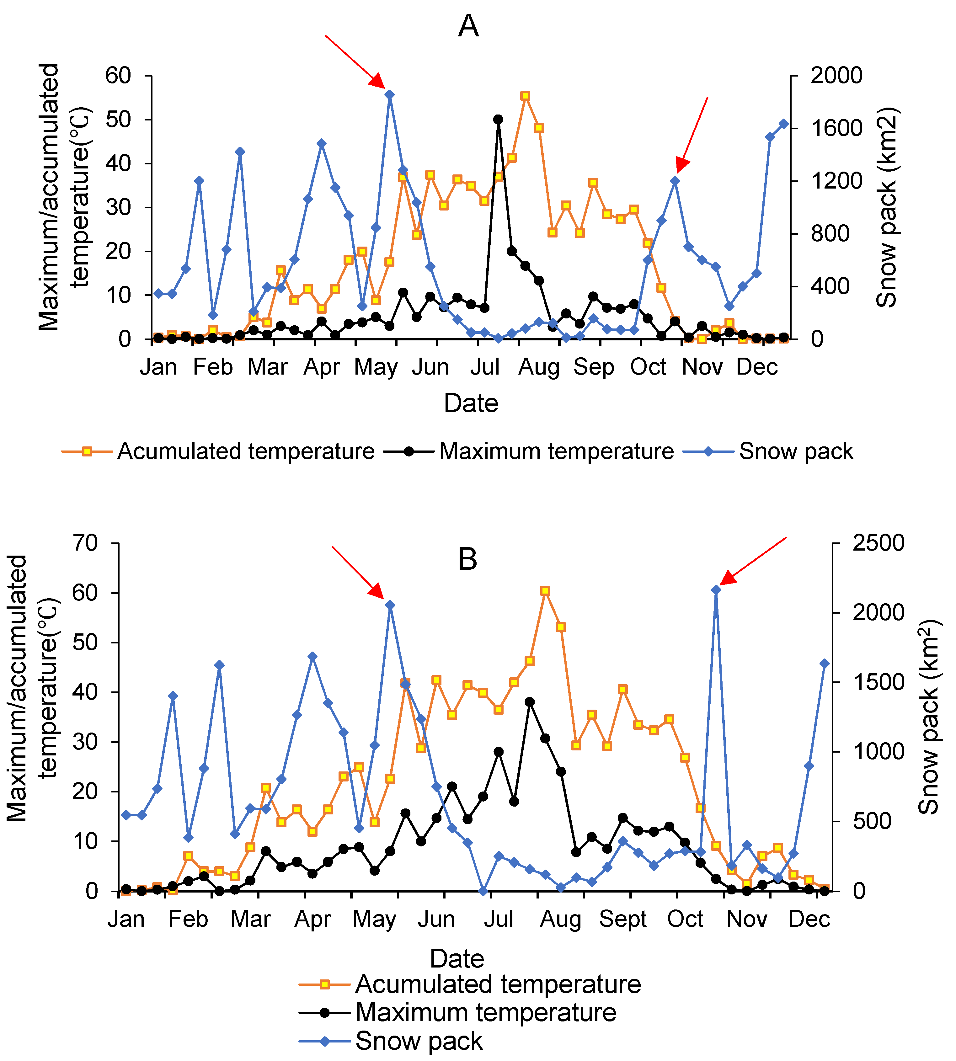
3.5. Comparison of Snow Pack Area and Temperature for the Selected Catchments

Analysis of the temperatures (maximum/accumulated) and remotely sensed snow packing of A and B catchments in 2015 was conducted (Figure 3). The eight-day range was the time taken for the snow pack measurements. The two arrows in Figure 3 indicate how the snow area’s turning points change throughout the year. For catchments A and B, the snow pack areas at the turning points from left to right were 1853.68 and 1200 km² and 2053.68 and 2164.76 km², respectively. For A, the first arrow was between May and June. The snow pack areas of both catchments began to decrease then. The snow-melting process started at this point denoted by the red arrow while the inflection point, which is the second turning point, started in early November. As the time between the first arrow (on the left) and the second arrow (on the right) contained temperatures that fit the conditions for rainfall, the snow pack obviously decreased, and the precipitation took the form of rain. When there was precipitation on a given day, the measured temperature conditions were compared to the values we were given. The daily average values of temperatures (maximum/accumulated) were used to determine the temperature conditions for snowfall during this time. Since the snow pack area increased as time approached the right arrow, for both catchments, snowfall clearly occurred (A and B).

3.6. Calibration and Validation

To improve the model’s simulation accuracy, the optimal parameter set was determined using parameter calibration. The study period was divided into three sections: warm-up period (2013–2014), calibration period (2015), and validation period (2016). The objective function was used to calibrate the simulated daily streamflow based on observations made at the Balykchy and Tossor stations, depending on the catchment’s location. The simulated results were evaluated using three statistical coefficients indices: the Nash–Sutcliffe efficiency (NSE) [74], goodness of fit (R²), and percent bias (PBIAS) [75]. The NSE is a metric that indicates how well the simulated and measured values match. The result is acceptable if the NSE value is between 0 and 1. The model’s performance is defined as “very good”, “good”, “satisfactory”, or “unsatisfactory” [75]. The NSE is calculated using the following formula:

$$\mathrm{NSE}=1-\frac{{{\displaystyle \sum }}_{\mathrm{i}=1}^{\mathrm{n}}{\left(Q_{obs,i}-Q_{sim,i}\right)}^2}{{{\displaystyle \sum }}_{\mathrm{i}=1}^{\mathrm{n}}{\left(Q_{obs,i}-{\overline{Q}}_{sim,i}\right)}^2};-\infty \le \mathrm{NSE}\le 1$$

(10)

The correlation between the simulated and measured values is expressed as R². It is calculated using the following formula:

$${\mathrm{R}}^2=\frac{{{\displaystyle \sum }}_{\mathrm{i}=1}^{\mathrm{n}}{\left[\left(Q_{sim,i}-{\overline{Q}}_{sim,i}\right)\left(Q_{obs,i}-{\overline{Q}}_{0bs,i}\right)\right]}^2}{\sqrt{{\mathsf{\Sigma }}_{\mathrm{i}=1}^{\mathrm{n}}{\left(Q_{sim,i}-{\overline{Q}}_{sim,i}\right)}^2{\mathsf{\Sigma }}_{\mathrm{i}=1}^{\mathrm{n}}{\left(Q_{obs,i}-{\overline{Q}}_{0bs,i}\right)}^2}}$$

(11)

The PBIAS value measures the average tendency of the simulated results to be higher or lower than the observations. The PBIAS is calculated using the following equation:

$$\mathrm{PBIAS}=\left(\frac{{{\displaystyle \sum }}_{\mathrm{i}=1}^{\mathrm{n}}{Q}_{sim,i}-{{\displaystyle \sum }}_{\mathrm{i}=1}^{\mathrm{n}}{Q}_{obs,i}}{{{\displaystyle \sum }}_{\mathrm{i}=1}^{\mathrm{n}}{Q}_{obs,i}}\right)$$

(12)

where $Q_{obs,i}$ is the measured discharge on the ith day (m³·s⁻¹); $Q_{sim,i}$ is the simulated discharge on the ith day (m³·s⁻¹); $Q_{sim,i}$ and $Q_{obs,i}$ are the average simulated and measured discharges during the simulation period (m³·s⁻¹), respectively; and n is the total number of daily flow observations.

4. Results

4.1. Rain and Snow Temperature Differences

Due to the sizes of the watersheds, temperature data from two corresponding stations could represent the temperature situation of the entire catchment (2153.46 km² and 2254.32 km²). The temperature conditions in relation to rainfall and snowfall for the years 2015–2016 have been measured (

Table 1. The temperature (°C) conditions of rain and snow in the study area. ACC.T means accumulated temperature and MAX.T means maximum temperature. Balykchy: 42.46 lat, 76.19 long; Tossor: 42.17 lat, 77.44 long.

Location	A				B
Average	Temperature for Rainfall		Temperature for Snowfall		Temperature for Rainfall		Temperature for Snowfall
	ACC.T	MAX.T	ACC.T	MAX.T	ACC.T	MAX.T	ACC.T	MAX.T
2015	39.12	16.42	28.51	14.84	27.91	11.94	29.4	12.5
2016	42.06	15.94	35.43	19.02	36.12	14.25	24.21	13.7
Average	40.59	16.18	31.97	16.93	32.01	13.09	26.80	13.1

). It is clear that rainfall occurs when ACCT reaches 40.59 or 31.97 °C with a MAXT of 16.18 or 13.095 °C for A and B, respectively. Snowfall occurs when ACCT is lower than 31.97 or 26.80 °C with a MAXT of 16.93 or 13.1 °C for A and B, respectively. During snowfall events on catchment A, the ACCT and MAXT cannot exceed 31.9 and 16.93 °C, respectively, and on catchment B, the ACCT and MAXT cannot exceed 26.805 and 13.1 °C, respectively. The two catchments experience differences in temperature conditions. The temperatures were higher in the northern catchment (A) than in the southern catchment (B). Catchments A and B are located in high mountains, Kungey Ala-Too and Teskey Ala-Too, at 3798 and 4762 m, respectively [76]. The temperatures of snowfall in high mountains are lower than those in low mountains [39,77]. From the Balykchy and Tossor stations, the different precipitation events were corrected. Using probability statistics for different precipitation type events at the two stations was considered to indicate the conditions of temperature linked to the precipitation events. Measured temperature conditions, all precipitation types, and simulated temperature conditions were compared. For the correct precipitation type, the temperature conditions needed to be the same. The proportion of the precipitation events that met that condition was used to show the accuracy. The accuracies were 79.45% and 84% for both catchments, given measurements from Balykchy and Tossor stations, respectively.

Sensitivity Analysis

The parameter sensitivity analysis for the original and updated SWAT models in SWAT-CUP, a SWAT model extension, is summarized in

Table 2. Parameter sensitivity analysis of the model for the chosen catchments.

A							B
Before Modification				After Modification			Before Modification			After Modification
No	Parameter	T-Test	p-Value	Parameter	T-Test	p-Value	Parameter	T-Test	p-Value	Parameter	T-Test	p-Value
1	SMTMP	0.05	0.85	SMTMP	0.04	0.95	SNO_SUB	0.24	0.81	SMTMP_accu	0.04	0.96
2	SNO_SUB	−0.08	0.81	TLAPS	0.04	0.94	SMTMP	−0.68	0.79	TLAPS	0.04	0.94
3	TLAPS	−0.32	0.75	SMTMP_accu	−0.1	0.90	SFTMP	−0.33	0.71	SFTMP_accu	−0.1	0.92
4	SNOCOVMX	−0.34	0.69	SFTMP_accu	0.14	0.89	SMFMX	−0.44	0.69	SNO_SUB	−0.15	0.87
5	SFTMP	−0.37	0.61	SFTMP	0.20	0.85	TLAPS	−0.47	0.61	PLAPS	0.20	0.86
6	SMFMX	0.50	0.59	SNO_SUB	0.24	0.80	SOL_AWC	0.48	0.58	SFTMP	0.24	0.81
7	PLAPS	−0.49	0.57	PLAPS	0.33	0.75	PLAPS	−0.58	0.57	SMTMP	0.33	0.79
8	SOL_AWC	0.83	0.41	SNOCOVMX	0.60	0.63	SNOCOVMX	0.61	0.40	SNOCOVMX	0.	0.71
9	ESCO	2.78	0.39	SMFMX	0.68	0.60	SMFMX	1.58	0.29	SMFMX	0.75	0.69
10	SMFMN	−0.79	0.03	SMFMN	0.77	0.57	SMFMN	−0.80	0.08	SMFMN	0.80	0.51

. SNO_SUB represents initial snow water content (mm H₂O), SNOCOVMX stands for minimum snow water content equal to 100% snow cover (mm), SOL_AWC is the soil evaporation compensation factor, SMFMX means melt factor for snow on June 21 (mm H₂O/°C-day), and ESCO stands for the soil evaporation compensation factor. When comparing the performance of the model before and after adjustment, the model was found to be less effective before adjustment. The original model’s p-values for catchments A and B were 0.03–0.85 and 0.81–0.08, respectively. The updated model’s p-values were 0.57–0.95 and 0.51–0.96, respectively.

4.2. Best Parameter Set

The parameters adjusted in the snow-melting route were analyzed (

Table 3. List of important parameters adjusted during calibration.

		CB		CA
Parameter Description	Unit	CV(A)	CV(B)	CV(A)	CV(B)
Snowfall temperature (SFTMP)	°C	3.67	4.5	3.89	4.68
Snowfall (SFTMP_accu)	°C	31.97	25.6	31.8	25.5
Snowmelt base temperature (SMTMP)	°C	2.42	3.8	2.69	3.89
Snowmelt base (SMTMP_accu)	°C	28.51	29.4	28.39	28.9
Melt factor for snow on 21 June (SMFMX)	mmH2O/°C-day	6.87	2.93	6.81	2.83
Melt factor for snow on 21 December (SMFMN)	mmH2O/°C-day	9.76	5.62	9.77	5.61
Temperature lapse rate (TPLAS)	°C.km−1	−7.46	2.32	−7.44	2.33
Precipitation lapse rate (PLAPS)	mm.km−1	24	21	25	22

CB: Calibration before modification, CA: Calibration after modification CV (A): Calibrated values (A), CV (B): Calibrated values (B).

). The ACCT thresholds for rainfall during model calibration (in 2015) were 39.12 and 27.91 °C for A and B, respectively. The ACCT thresholds for snowmelt were 28.51 and 29.4 °C for A and B, respectively. The parameters were set to different values during the calibration process. Some parameters, such as groundwater and soil, were omitted because they played a minor role in model calibration. The temperature of snow melting was one of the most important parameters.

4.3. SWAT Model Performance

The statistical coefficients (NSE, R², and PBIAS) were determined and used to indicate the accuracy of the model (during calibration and validation) by comparing the observed and simulated daily streamflow of the catchments before and after modifying the model (

Table 4. Statistical coefficients calculated to verify the model’s accuracy for the catchment A.

	Before Modification			After Modification
	NSE	R2	PBIAS (%)	NSE	R2	PBIAS (%)
Calibration	0.72	0.73	2.56	0.80	0.84	1.51
Validation	0.67	0.69	1.24	0.79	0.79	−2.2
Overall	0.64	0.72	5.75	0.75	0.87	4.31

and

Table 5. Statistical coefficients calculated to verify the model’s accuracy for the catchment B.

	Before Modification			After Modification
	NSE	R2	PBIAS (%)	NSE	R2	PBIAS (%)
Calibration	0.69	0.74	4.71	0.75	0.75	3.79
Validation	0.73	0.73	1.02	0.79	0.81	0.94
Overall	0.61	0.75	6.5	0.69	0.86	4.97

). The simulation period was from 2013 to 2016; the warmup period was from 2013 to 2014; and the calibration and validation periods were 2015 and 2016, respectively. The periods were chosen based on observation discharge data.

After model modification, there was improvement of the statistical values, which were used to verify the accuracy of the model for the catchments (Table 4 and Table 5). Overall, differentiation of snowfall and rainfall, along with the modified degree-day factor, may cause PBIAS to increase or decrease [37]. The statistical values improved significantly after the model was updated. As a result, it should be stated that modifications made to the SWAT model improved its performance. In general, the SWAT model was upgraded due to the enhancement of the snowmelt module.

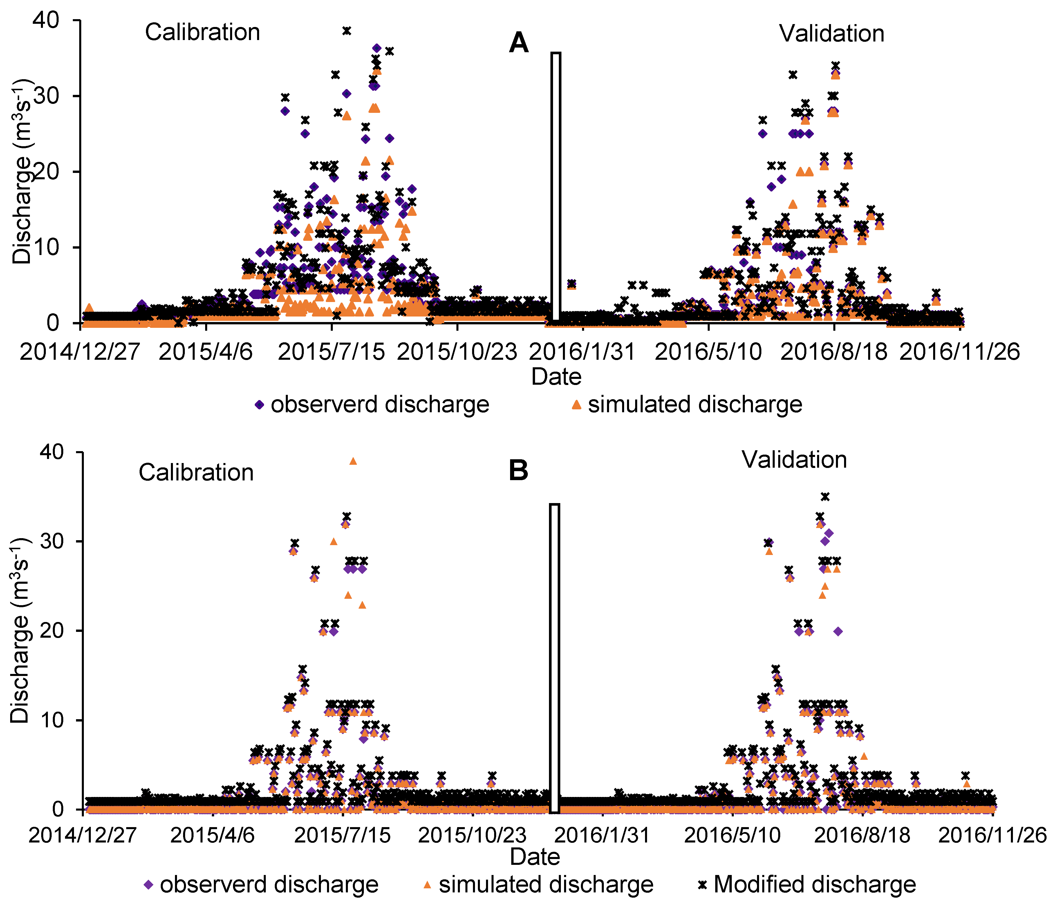
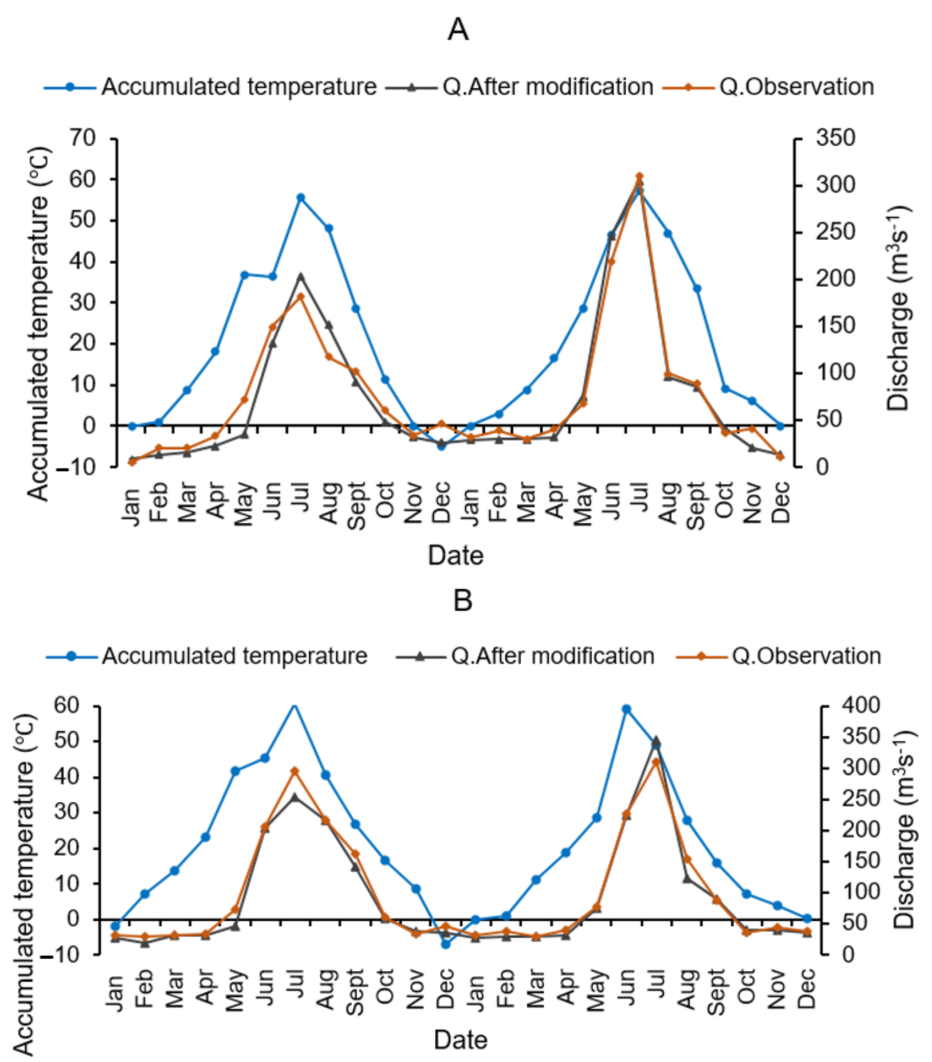
4.3.1. Stream Flow in the Catchments

For both catchments (A and B), a comparison of observed and simulated discharges before and after model adjustment was conducted (Figure 4). During the winter months (October to March), the mean observed daily discharges for catchments A and B were 2.2 and 1.91 m³·s⁻¹, respectively. The simulated discharges before model modification were 1.89 and 2.4 m³·s⁻¹ for catchments A and B, respectively; and after model modification, they were 4.3 and 3.9 m³·s⁻¹. Before, the model underestimated the peaks. After model modifications, some peaks were overestimated, and others remained unchanged, especially during the snowmelt periods (April to September) during the calibration and validation periods. The mean observed daily discharges for catchments A and B were 12.3 and 11.34 m³·s⁻¹, respectively, and the mean simulated discharges before and after model modification were 10.23 and 14.13 m³·s⁻¹ for catchment A and 11.67 and 13.43 m³·s⁻¹ for catchment B during these seasons. In general, the model’s simulated discharge was closer to the observed discharge before modification. After modification, the model estimated more flood peaks compared to the peaks estimated before modification (Figure 4), which could indicate the likelihood of flood occurrence due to snow in high mountains causing flooding. The shifting time of peak appearing time (S.T) and error of peak flood (E.F: between observed and simulated discharges during calibration and validation periods) were calculated. The maximum value of the peak flood appeared in July for both catchments. The S.T values were 2.14 and 0.95–1 days for A and B, respectively; E.F accounted for –2.12 and –0.39% for A and B, respectively. This is consistent with the findings of [37,78], who also stated that, occasionally, there is a “one peak, one day” flood phenomenon, which helps peak selection analysis. During calibration and validation, the arrangement of the 16 high peaks for each catchment was analyzed. The average peak flows after model modification in catchments A and B were 12 and 10% higher than the average of peak flows before model modification. It is indicated by the peaks provided in different colors for the simulated, observed, and modified discharge (Figure 4). This made the peaks become closer to their corresponding observation discharges. This suggests that upgrading the snowmelt module can result in more accurate model simulations, which is indicated by statistical values (Table 4 and Table 5).

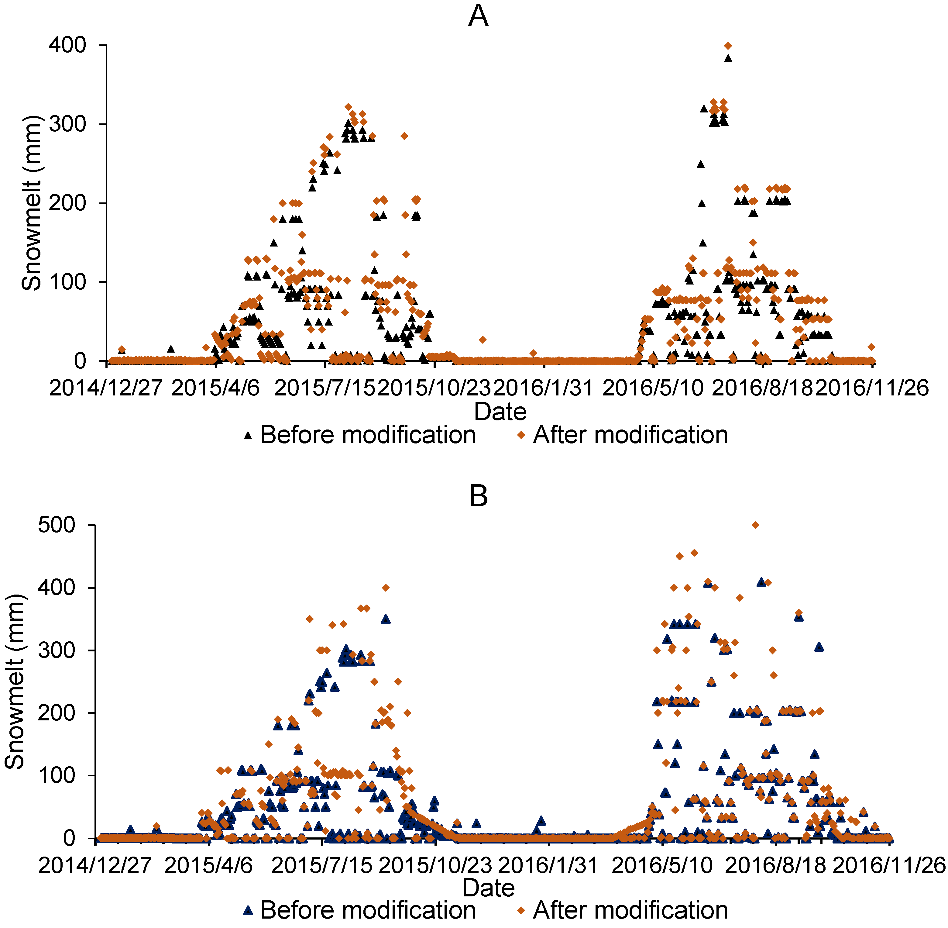
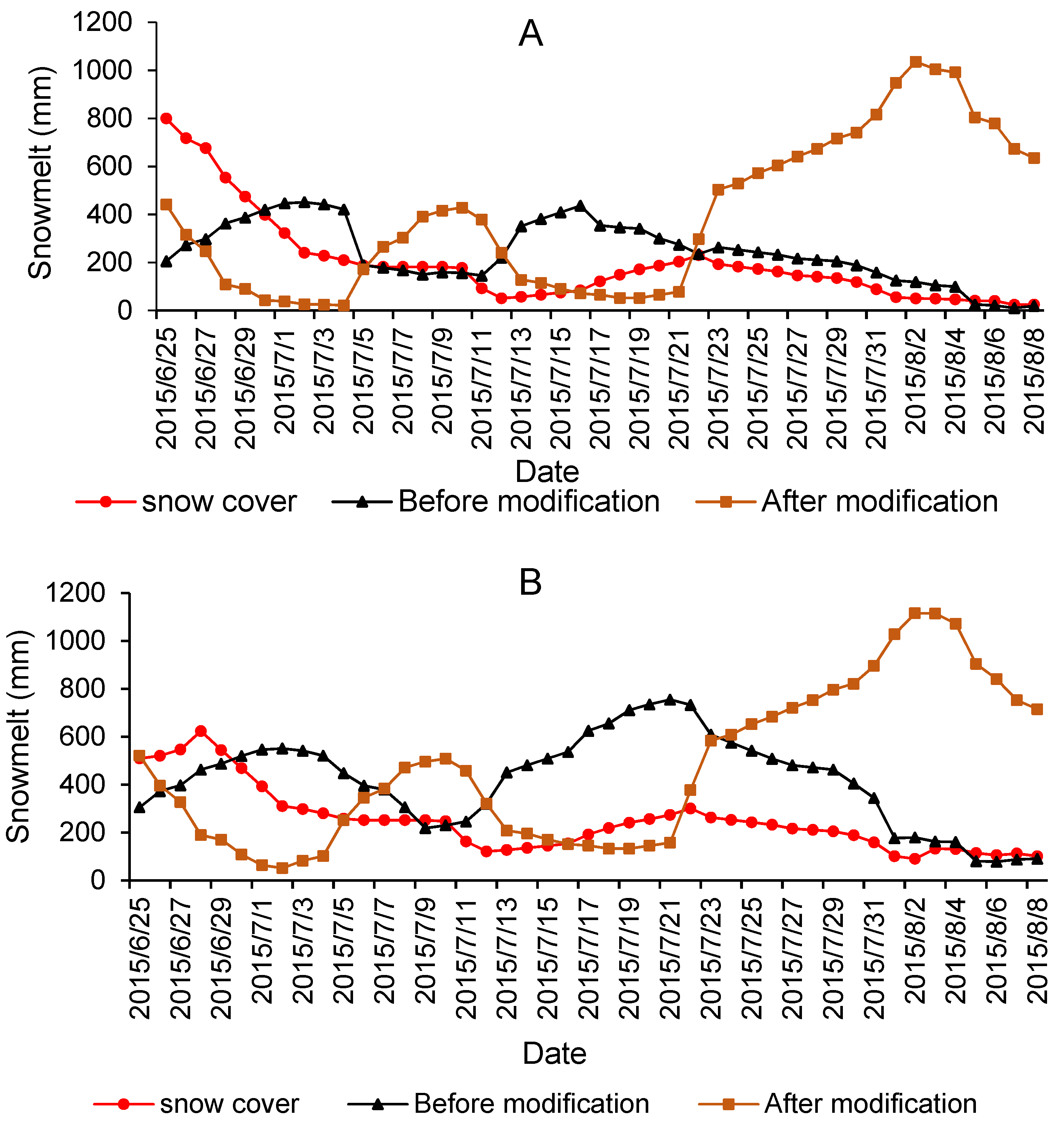
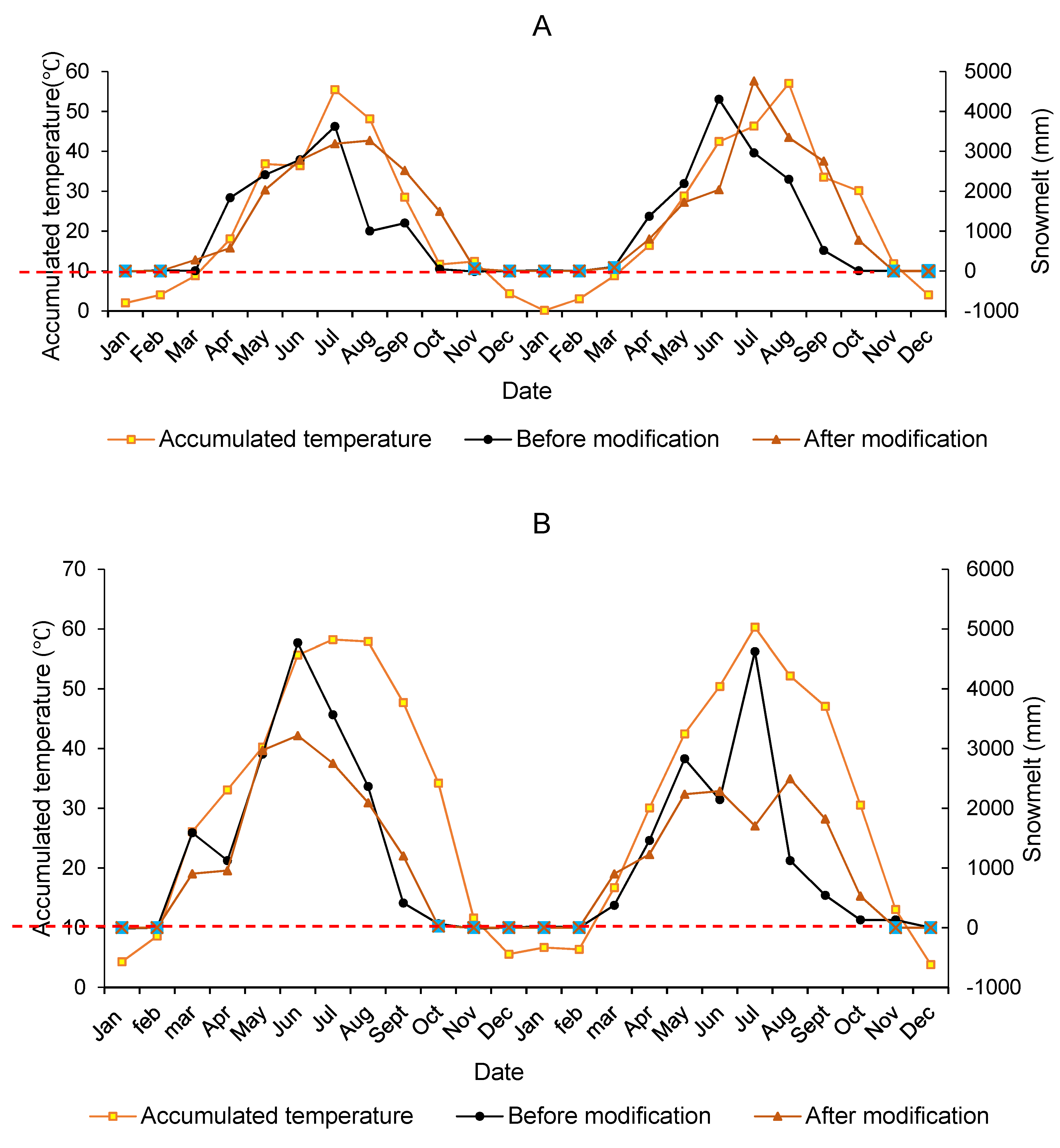
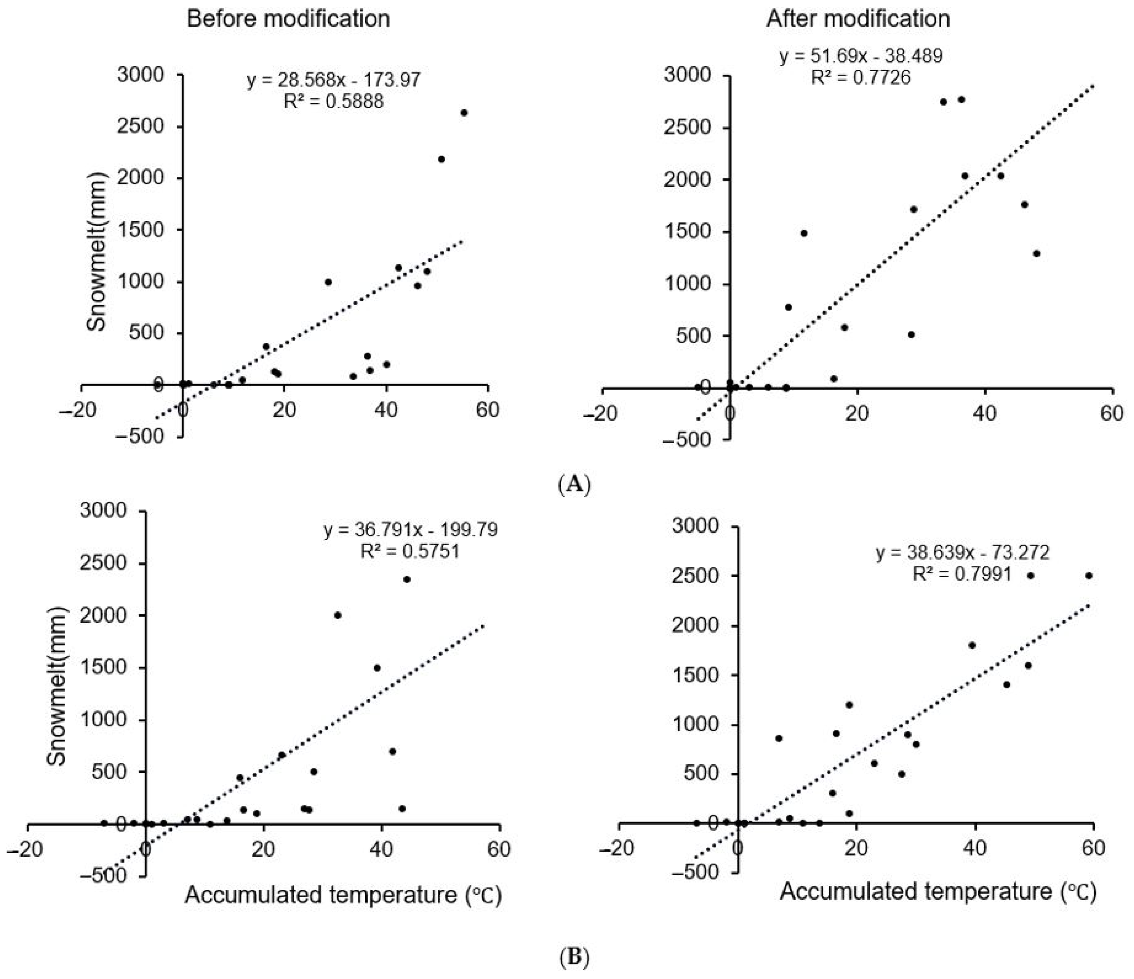
4.3.2. Accumulation Temperature and Snowmelt

The degree-day factor method engaged in SWAT is an important approach for calculating snow and ice melt [79,80]. A comparison of daily snowmelt before and after model modification was conducted (Figure 5). This snowmelt stream flow simulation approach matches the characteristics of the snowmelt floods in the watersheds surrounding the Issyk-Kul Lake. The daily average snowmelt amounts for catchments A and B were 43.01 and 46.14 mm, respectively, and after model modification, they were 37.36 and 45.20 mm reductions of 13.12 and 2.03%. However, prior to model modification, the amount of snowmelt by considering flood peaks were 122.45 and 134.27 mm for A and B, respectively. After model improvement, the snowmelt amounts for A and B were 129.8 and 143.67 mm, respectively. After modifying the model, the increases were about 6 and 7% for A and B, respectively. These results revealed that the simulated snowmelts were significantly higher in the spring and summer when using the modified model (high frequency in spring). Snowmelt is obviously more pronounced in high mountains with snow and ice, causing floods; similar findings have been found by [16] and in neighboring regions [37]. Some exceptions, such as snowmelt obtained using the original model, were neglected. Before the modifications, runoff contributed 45.3 and 40.67% to catchments A and B, respectively, which then became 56.29 and 53.26% for A and B.

The relationship between the amount of eight-day snowmelt and the snow cover during melting periods was investigated. The model’s rationality before and after modification and snowmelt calculations were revealed too (Figure 6). For all catchments in August, the volume of snowmelt calculated after modification showed an increasing trend that tended towards strong matching of the peaks, whereas before modification, there was a decreasing trend. In general, the snow cover decreased in summer, owing to the high temperatures. As indicated by the peaks that form a circle for a few days, the snow cover can increase for a short period of time, which corresponds to a rapid decrease and then increase in temperature. According to the findings, the model’s performance after modification was better. This is also indicated by how the modified model’s trend was an increasing one, whereas the original model’s trend decreased in Figure 6, more especially in August. Sudden changes in a short period of time, according to [81], can result in intense runoff, which can cause flooding. The modified model revealed the characteristics of floods in the area.

The relationships between ACCT and MAXT and monthly snow melting during the calibration (2015) and verification periods (2016) are presented in Figure 7. When the accumulated temperature in the selected catchments reaches 10 °C, the snow melts. The crosses denote non-melting months; normally, there is no snowmelt from November to February. Prior to the introduction of the degree-day though, the model indicated some amount of snowmelt in the non-melting months; however, after modification, there was no snowmelt found in those months, making snowmelt more accurate and reasonable. The cumulative temperature threshold of snow melting was reached between January and March in 2016 and November and December of the same year.

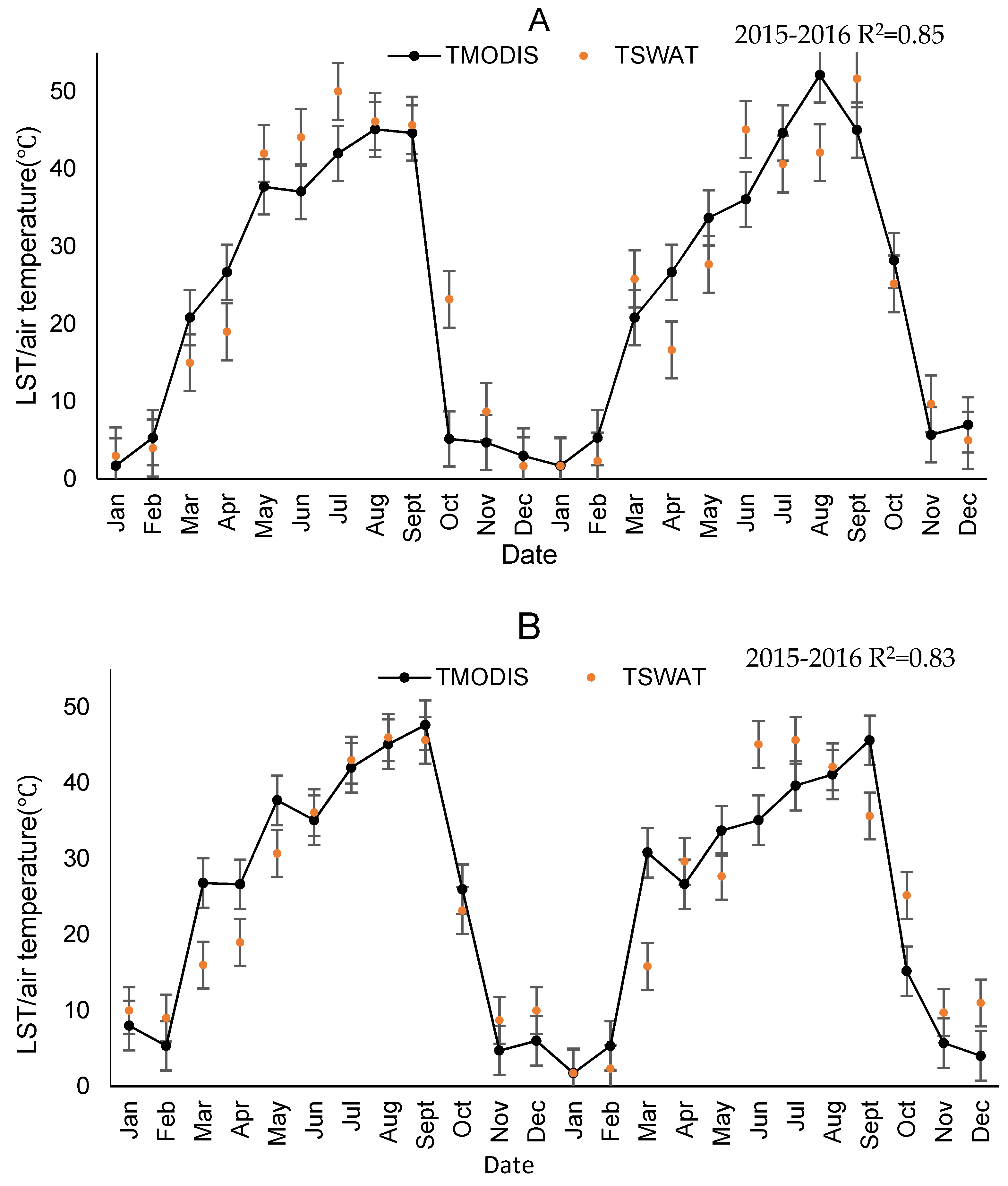
4.4. Land Surface and Air Temperatures

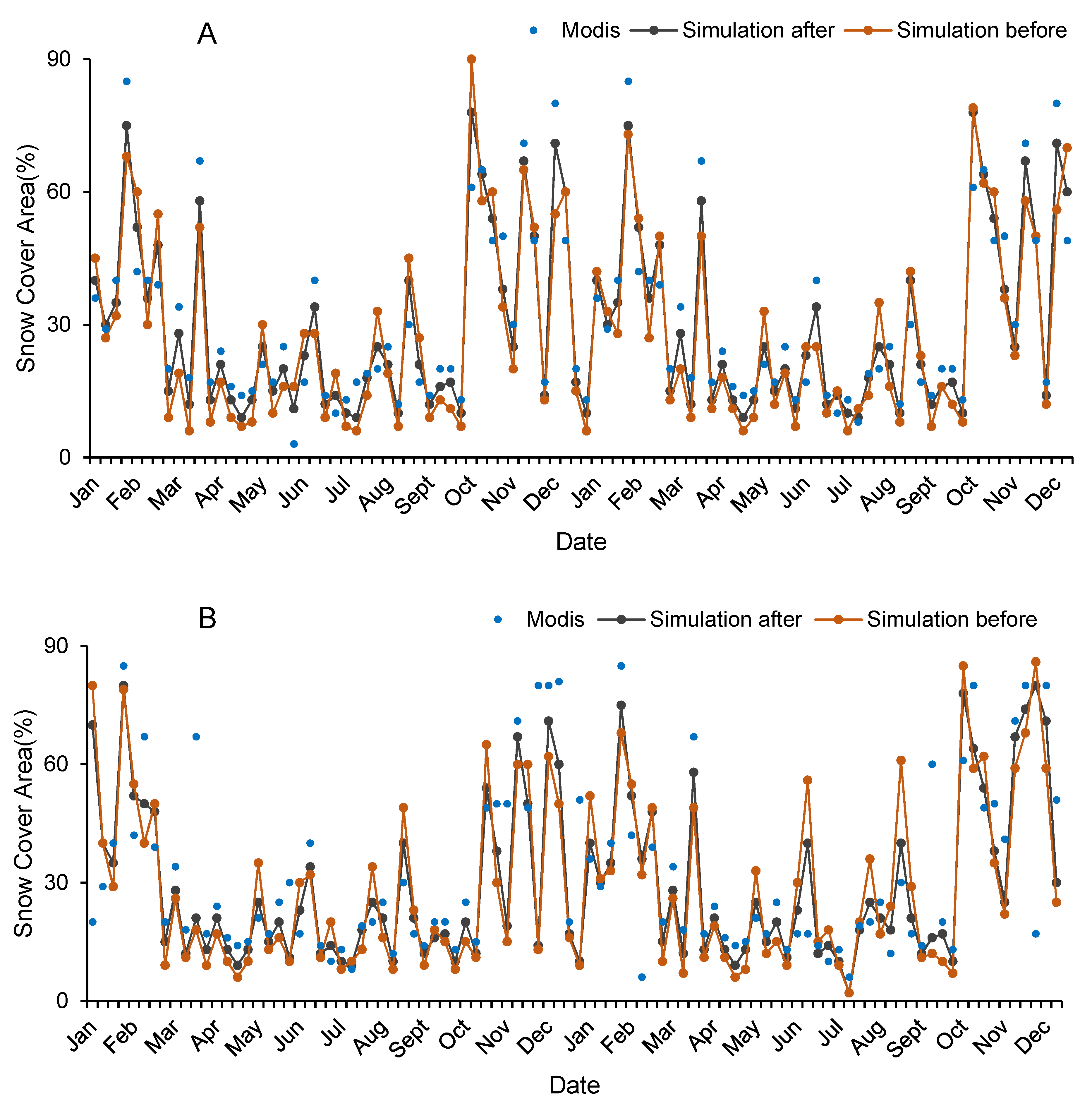
Simulation of Snow Cover Area

To validate the modeled snow cover, simulated results of snow cover area and data of MODIS (Figure 8) were compared during the calibration and verification periods, 2015 and 2016, respectively. During the calibration period, the snow cover area reached a lower value in summer and the MODIS data overestimated the value in later and earlier spring for catchments A and B, respectively. In general, in spring and summer during calibration and validation, the snow cover area tended to decrease, and in non-melting periods, the area increased.

The results of a linear regression analysis of the relationship between snowmelt and ACCT are presented in Figure 9. Snow is sensitive to temperature, and snow accumulation in the area is concentrated in the high-altitude regions [82]. On the surface of snow cover, the temperature drives the melting process. The modified model performed better with R² = 0.762 and 0.757 for A and B, respectively. However, after the model was modified, the correction was relatively low, with R² = 0.506 and 0.515 for A and B, respectively. Based on our results, it can be concluded that modifying the SWAT model, particularly using the degree-day factor method, is highly effective for snowmelt analysis and prediction.

The average monthly land surface temperatures (LST) of MODIS were calculated and compared to air temperatures of the SWAT model from 2015 to 2016. To validate the air temperatures used in the model, the land surface temperatures within elevation bands of the whole catchments were calculated and were compared with the air temperatures. The R² values were 0.85 and 0.83 for A and B catchments, respectively, (Figure 10). These statistical values indicate that the used air temperature in the model was sufficient for the simulations. Furthermore, a comparison between discharge and accumulated temperature has been undertaken to better understand the relationship between the two (Figure 11). The findings demonstrated that as the accumulated temperature rises in the spring and summer, so does the overall discharge.

5. Discussion

This study proposed a method for estimating the snowmelt degree-day factor based on MODIS snow cover data. In the selected catchments, the spatial distribution of the degree-day factor method was estimated and attributed to the interactions of climate conditions, topography, and vegetation. The estimated degree-day factor values were 4.7 and 4.3 mmH₂/°C for A and B, respectively, which are within the ranges of 3.1–5.9 mmH₂/°C [43] and 4.3–5 mmH₂/°C [83]. These values are also close to the range of 5.0–11.6 mmH₂/°C found by studies in the Himalayas [3,4]. The simulations using the modified degree-day factor method on runoff in terms of discharge and volume of snowmelt are more plausible than the original model, pre-modification. They were influenced by a variety of hydrological processes, along with the interactions of the hydrological model parameters [84]. The SWAT model ignores the possibility of snowfall and calculates precipitation as rain [85]. This may reduce snowmelt runoff and increase rainfall. The modeling scale can have a significant influence on the simulations, considering the spatial resolution of MODIS data for precipitation and temperature [86]. The temperature threshold values determine the occurrence of snowmelt in mountain basins. This is in line with the study by [87], who stated that the accumulation temperature is the driving force for triggering the snowmelt. The results revealed that the temperature threshold of the catchment located in the northwest of Issyk-Kul was 4.89% higher than the threshold of the catchment located in the south of the lake, due to elevation differences, topography, and water vapor conditions; this is consistent with [37]. The lower the elevation, the more accurate the rain and snow estimations [88]. Changes in climate conditions in high mountains affect the correctness. In the SWAT model, the daily maximum and minimum temperatures are used, but there is a difference between land surface temperature and air temperature [89]. Temperature variations in a single day can be classified into three main parts: the maximum daily temperature is below 0 °C; the maximum daily temperature is above 0 °C, but the minimum daily temperature is less than 0 °C; and the minimum daily temperature is greater than 0 °C [90]. It is preferable to use land surface temperature to calculate snowmelt [91,92]. In this context, for this study, the differences in air and ground temperatures were taken into account [37]. When observations of precipitation are corrected from meteorological stations, the precipitation types are always the same [93], except that the temperature threshold is set to determine the precipitation type when passing observation values into the SWAT model [94,95]. The catchment’s area is enough for their components to be verified. The accumulated and maximum temperatures were improved, and then the snow and rain accuracies were verified, as part of a model modification process, to improve its performance. Furthermore, the optimal accumulated and maximum temperatures were achieved, and the accuracies of precipitation type and snowmelt measurements were modified. The use of average temperature as a criterion for snowmelt has an impact on snowmelt volume computation [37,96]. The process of surface temperature accumulation can then be well represented, improving calculation accuracy, by using both the accumulated and maximum temperatures in the snow-melting calculation.

5.1. Model Performance

The statistical coefficients before and after model modification were calculated (Table 4 and Table 5). For all catchments, the simulation results obtained after modification were better than before. The PBIAS values from verification using the modified model were better than that of the model before (Table 4 and Table 5). The temperatures in Issyk-Kul’s northern and southern catchments begin to rise in early April, snow begins to melt into stream flow, and the water levels in the catchments begin to rise rapidly [25], eventually leading to floods [97,98,99]. Our results showed that the participation of snowmelt from October to March was limited to the modified degree-day method, which increased from April to September. In fact, the method brought the observed discharge closer to the simulated values (Figure 2). During simulations, the differentiation between rain and snow in terms of precipitation for all catchments increased snowmelt and decreased rainfall in proportion to runoff, which matches our findings from a simulation conducted in the Xinjiang region’s Kunlun Mountains [40]. Rainfall in the catchments is scarce, and the increase in the runoff from April to September is due to snowmelt, as described by [16,48]. Flooding was predicted by the modified model to occur during the spring. The temperature, which causes snow to melt, increases in summer [100]. To evaluate the discharge, the shifting time of peak appearing time and the error of peak flood were considered. Most of the high peaks occurred during spring and winter.

The modified model performed better than the original model; the peaks of flood flow increased, bringing the discharge closer to the measured values. The northwestern catchment of Issyk-Kul indicated lower discharge compared to the southern catchment for the study period, probably due to differences in location, elevation, and catchment area. For catchment A, the average daily flow in 2015 was 25.72 m³·s⁻¹, which was lower than 35.12 m³·s⁻¹ in 2016. In 2015, the average daily flow into catchment B was 39.04 m³·s⁻¹, which was lower than 41.83 m³·s⁻¹ in 2016. These differences could be due to both climate change and human activities [16]. Furthermore, variations in runoff in catchments are primarily caused by changes in climate [76]. The contributions of snowmelt to the water flow were approximately 6 and 7% greater for catchments A and B, respectively, according to the modified model compared to the original model. The Sequential Uncertainty Fitting (SUFI-2) algorithm [101] considers uncertainties in observation data, parameters, model structure, and input data. After consideration, the algorithm determines the impacts of the parameters and puts them in ranges. The sensitivity parameters were ranked before and after modification for both models. To improve the model’s performance, the parameters related to snowmelt were modified. In the traditional and modified models, the parameters of snowmelt base temperature SMTMP for catchment A, initial snow water content (mm H₂O) (SNO_SUB) for catchment B, (SMTMP_accu) for catchment A, and snowmelt base temperature (SMTMP_accu) for catchment B showed strong sensitivity. Before and after model modification, the parameter of melt factor for snow on December 21 (SMFMN) showed a low sensitivity for both catchments. Because of differences in input data, the snowmelt module in the modified model of catchment A performed better than the modified model for catchment B. Generally, the entire snowmelt module in both selected catchments’ original models indicated a low response during the calibration process. Thus, model modification for the snowmelt module improved the model’s results by increasing accuracy and reliability.

5.2. Accumulation Temperature and Snowmelt

The precipitation within the HRU is labeled as snow if the mean daily air temperature falls below the boundary temperature and the snow equivalent is applied to the snow pack. When snowfall accumulates on the ground surface, it forms a snow pack. The amount of water contained in the snow pack is measured in snow water equivalents. Additionally, snowfall will increase the snow pack, whereas snowmelt or sublimation will reduce it. During simulation, the traditional degree-day factor method only uses average temperature in calculations [99], but after adding accumulation temperature, the model performed better in melt seasons simulations. The temperatures were higher in the northern catchment (A) than in the southern catchment (B). This is due to altitude differences and the wet air from Issyk-Kul. The increase in elevation causes air pressure to decrease; hence, air molecules are further apart, causing the temperature decreases [1,2,3]. The snow melts when certain accumulated and maximum temperatures are reached, which can happen in a single day. The modified model simulated more flood peaks in the simultaneous snowmelt floods and rainfall floods that occur during melting seasons. The accumulated threshold for all catchments was 10 °C (Figure 7), which improved the snowmelt calculations. There was some inconsistency between the simulated discharge before the model modification during melt seasons and non-melt seasons for all catchments, but the model modification eliminated the errors. After model modification, the results showed higher snowmelt peaks during snowmelt seasons (summer), and the amount of snowmelt was increased for all catchments (Figure 5). This means that upgrading the snow melt module led to an increase in the amount of snowmelt, which shows that the model made a significant improvement after the modifications. Our results look quite similar to the results obtained by [37].

6. Conclusions

In this study, a new algorithm was used to calculate snowmelt in the catchments around Issyk-Kul in SWAT. The model was able to simulate the discharge and snowmelt. It needs to be calibrated and validated. The existence of the degree-day factor method and the precipitation type differentiation in the model were highlighted. The modifications seemed to improve the snowmelt module of the model. Through the improvement of the module, the sensitivity of the snowmelt-related parameters was been greatly improved. To improve the accuracy of the original model, the accumulation of temperature conditions was determined. During the calibration process, the modified model was used to calculate the discharges in the catchments. Through model modification, the degree day factor method calculated snow melt, and the snow-related parameters were calibrated manually; the statistical values such as NSE and R² were improved. The NSE increased from 0.72 to 0.80 and from 0.69 to 0.75 for catchments A and B, respectively. R² increased from 0.73 to 0.84 and from 0.74 to 0.75 for A and B, respectively (Table 4 and Table 5). The shifting times were 2.14 and 0.95–1 days for A and B, respectively. Errors of peaks accounted for −2.12 and −0.39% for A and B, respectively. These results indicated that the model was good enough to simulate the discharge. After modifying the model, the flood peaks increased for A and B by 49.42 and 43.87%, respectively, bringing them closer to the reality of the observation discharge. This was more consistent with the characteristics of floods caused by snowmelt in the catchments around Issyk-Kul. The contributions of snowmelt to stream flow increased by 24.26 and 31% for A and B, respectively. Therefore, it is possible to limit snowmelt to reasonable times of the year by improving the traditional degree-day factor method with the addition of accumulated temperature conditions, while avoiding non-melting seasons. Finally, when using the model for mountainous regions, it is best to improve the degree-day factor method to improve accuracy. Differentiating precipitation and flood types may provide reliable information for flood forecasting, allowing for the identification of hazards and appropriate adaptive measures.

References

1. Rasool, S. Climate change, Global change: What is the difference? Eos Trans. Am. Geophys. Union 1988, 69, 668. [Google Scholar] [CrossRef]
2. Lin, N.-F.; Tang, J.; Han, F.-X. Eco-environmental problems and effective utilization of water resources in the Kashi Plain, western Terim Basin, China. Hydrogeol. J. 2001, 9, 202–207. [Google Scholar] [CrossRef]
3. Ji, X.; Kang, E.; Chen, R.; Zhao, W.; Zhang, Z.; Jin, B. The impact of the development of water resources on environment in arid inland river basins of Hexi region, Northwestern China. Environ. Geol. 2006, 50, 793–801. [Google Scholar] [CrossRef]
4. Michel-Guillou, E. Water resources and climate change: Water managers’ perceptions of these related environmental issues. J. Water Clim. Chang. 2015, 6, 111–123. [Google Scholar] [CrossRef]
5. Chen, Y.; Li, Z.; Fang, G.; Deng, H. Impact of climate change on water resources in the Tianshan Mountians. Cent. Asia. Acta Geogr. Sin. 2017, 72, 18–26. [Google Scholar]
6. Fischer, A. Glaciers and climate change: Interpretation of 50 years of direct mass balance of Hintereisferner. Glob. Planet. Chang. 2010, 71, 13–26. [Google Scholar] [CrossRef]
7. Gascoin, S.; Kinnard, C.; Ponce, R.; Lhermitte, S.; Macdonell, S.; Rabatel, A. Glacier contribution to streamflow in two headwaters of the Huasco River, Dry Andes of Chile. Cryosphere 2011, 5, 1099–1113. [Google Scholar] [CrossRef] [Green Version]
8. Pelto, M.S. Quantifying Glacier Runoff Contribution to Nooksack River, WA in 2013-15. In Proceedings of the 2015 AGU Fall Meeting Abstracts, San Francisco, CA, USA, 14–18 December 2015. [Google Scholar]
9. Swick, M.; Kaspari, S. Partitioning the Contribution of Light Absorbing Aerosols to Snow and Glacier Melt Using a Novel Hyperspectral Microscopy Method. In Proceedings of the 2017 AGU Fall Meeting Abstracts, New Orleans, LA, USA, 11–15 December 2017. [Google Scholar]
10. Hock, R.; Rees, G.; Williams, M.W.; Ramirez, E. Contribution from glaciers and snow cover to runoff from mountains in different climates. Hydrol. Process. 2006, 20, 2089–2090. [Google Scholar] [CrossRef]
11. Luo, Y.; Arnold, J.; Liu, S.; Wang, X.; Chen, X. Inclusion of glacier processes for distributed hydrological modeling at basin scale with application to a watershed in Tianshan Mountains, northwest China. J. Hydrol. 2013, 477, 72–85. [Google Scholar] [CrossRef]
12. Li, X.; Ma, Y.; Sun, Y.; Gong, H.; Li, X. Flood hazard assessment in Pakistan at grid scale. J. Geo-Inf. Sci. 2013, 15, 314–320. [Google Scholar] [CrossRef]
13. Lian, J.; Gong, H.; Li, X.; Zhao, W.; Hu, Z. Design and development of flood/waterlogging disaster risk model based on Arcobjects. J. Geo-Inf. Sci. 2009, 11, 376–381. [Google Scholar] [CrossRef]
14. Long, H.; Liu, Y.; Li, X.; Chen, Y. Building new countryside in China: A geographical perspective. Land Use Policy 2010, 27, 457–470. [Google Scholar] [CrossRef]
15. Zhao, G.; Pang, B.; Xu, Z.; Wang, Z.; Shi, R. Assessment on the hazard of flash flood disasters in China. J. Hydraul. Eng. 2016, 47, 1133–1142. [Google Scholar]
16. Alymkulova, B.; Abuduwaili, J.; Issanova, G.; Nahayo, L. Consideration of water uses for its sustainable management, the case of Issyk-Kul Lake, Kyrgyzstan. Water 2016, 8, 298. [Google Scholar] [CrossRef] [Green Version]
17. Giralt, S.; Klerkx, J.; Riera, S.; Julia, R.; Lignier, V.; Beck, C.; De Batist, M.; Kalugin, I. Recent paleoenvironmental evolution of Lake Issyk-Kul. In Lake Issyk-Kul: Its Natural Environment; Springer: Berlin/Heidelberg, Germany, 2002; pp. 125–145. [Google Scholar]
18. Vollmer, M.K.; Weiss, R.F.; Schlosser, P.; Williams, R.T. Deep-water renewal in Lake Issyk-Kul. Geophys. Res. Lett. 2002, 29, 124-1–124-4. [Google Scholar] [CrossRef]
19. Dawadi, S.; Ahmad, S. Changing climatic conditions in the Colorado River Basin: Implications for water resources management. J. Hydrol. 2012, 430, 127–141. [Google Scholar] [CrossRef]
20. Abadi, L.S.K.; Shamsai, A.; Goharnejad, H. An analysis of the sustainability of basin water resources using Vensim model. KSCE J. Civ. Eng. 2015, 19, 1941–1949. [Google Scholar] [CrossRef]
21. De Batist, M.; Imbo, Y.; Vermeesch, P.; Klerkx, J.; Giralt, S.; Delvaux, D.; Lignier, V.; Beck, C.; Kalugin, I.; Abdrakhmatov, K. Bathymetry and sedimentary environments of Lake Issyk-Kul, Kyrgyz Republic (Central Asia): A large, high-altitude, tectonic lake. In Lake Issyk-Kul: Its Natural Environment; Springer: Berlin/Heidelberg, Germany, 2002; pp. 101–123. [Google Scholar]
22. Jailoobayev, A.; Neronova, T.; Nikolayenko, A.; Mirkhashimov, I. Water Quality Standards and Norms in Kyrgyz Republic; Regional Environmental Centre for Central Asia (CAREC): Almaty, Kazakhstan, 2009. [Google Scholar]
23. Wang, G.; Shen, Y.; Wang, N.; Wu, Q. The effects of climate change and human activities on the lake level of the Issyk-Kul during the past 100 years. J. Glaciol. Geocryol. 2010, 32, 1097–1105. [Google Scholar]
24. Narama, C.; Shimamura, Y.; Nakayama, D.; Abdrakhmatov, K. Recent changes of glacier coverage in the western Terskey-Alatoo range, Kyrgyz Republic, using Corona and Landsat. Ann. Glaciol. 2006, 43, 223–229. [Google Scholar] [CrossRef] [Green Version]
25. Alifujiang, Y.; Abuduwaili, J.; Ge, Y. Trend Analysis of Annual and Seasonal River Runoff by Using Innovative Trend Analysis with Significant Test. Water 2021, 13, 95. [Google Scholar] [CrossRef]
26. Jost, G.; Moore, R.D.; Weiler, M.; Gluns, D.R.; Alila, Y. Use of distributed snow measurements to test and improve a snowmelt model for predicting the effect of forest clear-cutting. J. Hydrol. 2009, 376, 94–106. [Google Scholar] [CrossRef]
27. Martinec, J.; Rango, A. Parameter values for snowmelt runoff modelling. J. Hydrol. 1986, 84, 197–219. [Google Scholar] [CrossRef]
28. Anderson, E.A. A Point Energy and Mass Balance Model of a Snow Cover; US Department of Commerce, National Oceanic and Atmospheric Administration: Silver Spring, MD, USA, 1976; Volume 19.
29. He, Z.; Parajka, J.; Tian, F.; Blöschl, G. Estimating degree-day factors from MODIS for snowmelt runoff modeling. Hydrol. Earth Syst. Sci. 2014, 18, 4773–4789. [Google Scholar] [CrossRef] [Green Version]
30. Jones, H.; Sochanska, W.; Stein, J.; Roberge, J.; Plamondon, A.; Charette, J. Snowmelt in a boreal forest site: An integrated model of meltwater quality (SNOQUAL1). In Acidic Precipitation; Springer: Berlin/Heidelberg, Germany, 1986; pp. 1485–1493. [Google Scholar]
31. Smith, M.B.; Korenʹ, V.; Zhang, Z.; Reed, S.M.; Seo, D.; Moreda, F.; Kuzmin, V.A. NOAA NWS Distributed Hydrologic Modeling Research and Development; NOAA Institutional Repository: Silver Spring, MD, USA, 2004.
32. Shimamura, Y.; Izumi, T.; Matsuyama, H. Remote sensing of areal distribution of snow cover and snow water resources in mountains based on synchronous observations of Landsat-7 satellite-A case study around the Joetsu border of Niigata prefecture in Japan. In Proceedings of the General Meeting of the Association of Japanese Geographers Annual Meeting of the Association of Japanese Geographers, Spring 2004, 29 July 2004; The Association of Japanese Geographers: Tokyo, Japan, 2004. [Google Scholar]
33. Herrero, J.; Polo, M.; Moñino, A.; Losada, M. An energy balance snowmelt model in a Mediterranean site. J. Hydrol. 2009, 371, 98–107. [Google Scholar] [CrossRef]
34. Feng, T.; Feng, S. An Energy Balance Snowmelt Model for Application at a Continental Alpine Site. Procedia Eng. 2012, 37, 208–213. [Google Scholar] [CrossRef] [Green Version]
35. Jost, G.; Moore, R.D.; Smith, R.; Gluns, D.R. Distributed temperature-index snowmelt modelling for forested catchments. J. Hydrol. 2012, 420, 87–101. [Google Scholar] [CrossRef]
36. Yu, W.; Zhao, Y.; Nan, Z.; Li, S. Improvement of snowmelt implementation in the SWAT hydrologic model. Acta Ecol. Sin. 2013, 33, 6992–7001. [Google Scholar]
37. Duan, Y.; Liu, T.; Meng, F.; Luo, M.; Frankl, A.; De Maeyer, P.; Bao, A.; Kurban, A.; Feng, X. Inclusion of modified snow melting and flood processes in the swat model. Water 2018, 10, 1715. [Google Scholar] [CrossRef] [Green Version]
38. Arnold, J.G.; Fohrer, N. SWAT2000: Current capabilities and research opportunities in applied watershed modelling. Hydrol. Process. Int. J. 2005, 19, 563–572. [Google Scholar] [CrossRef]
39. Fontaine, T.; Cruickshank, T.; Arnold, J.; Hotchkiss, R. Development of a snowfall–snowmelt routine for mountainous terrain for the soil water assessment tool (SWAT). J. Hydrol. 2002, 262, 209–223. [Google Scholar] [CrossRef]
40. Xu, C.; Chen, Y.; Hamid, Y.; Tashpolat, T.; Chen, Y.; Ge, H.; Li, W. Long-term change of seasonal snow cover and its effects on river runoff in the Tarim River basin, northwestern China. Hydrol. Process. Int. J. 2009, 23, 2045–2055. [Google Scholar] [CrossRef]
41. ZHANG, X.-y.; Li, J.; Yang, Y.-Z.; You, Z. Runoff Simulation of the Catchment of the Headwaters of the Yangtze River Based on SWAT Model. J. Northwest For. Univ. 2012, 5. [Google Scholar]
42. Arnold, J.G.; Muttiah, R.S.; Srinivasan, R.; Allen, P.M. Regional estimation of base flow and groundwater recharge in the Upper Mississippi river basin. J. Hydrol. 2000, 227, 21–40. [Google Scholar] [CrossRef]
43. Zhang, Y.; Liu, S.; Ding, Y. Spatial variation of degree-day factors on the observed glaciers in western China. Acta Geogr. Sin. 2006, 61, 89. [Google Scholar] [CrossRef] [Green Version]
44. Zhang, Y.; Suzuki, K.; Kadota, T.; Ohata, T. Sublimation from snow surface in southern mountain taiga of eastern Siberia. J. Geophys. Res. Atmos. 2004, 109, D21. [Google Scholar] [CrossRef] [Green Version]
45. Arnold, J.; Allen, P.; Volk, M.; Williams, J.; Bosch, D. Assessment of different representations of spatial variability on SWAT model performance. Trans. ASABE 2010, 53, 1433–1443. [Google Scholar] [CrossRef]
46. Wang, X.; Melesse, A. Evaluation of the SWAT model’s snowmelt hydrology in a northwestern Minnesota watershed. Trans. ASAE 2005, 48, 1359–1376. [Google Scholar] [CrossRef]
47. Kumar, M.; Marks, D.; Dozier, J.; Reba, M.; Winstral, A. Evaluation of distributed hydrologic impacts of temperature-index and energy-based snow models. Adv. Water Resour. 2013, 56, 77–89. [Google Scholar] [CrossRef]
48. Hock, R. A distributed temperature-index ice-and snowmelt model including potential direct solar radiation. J. Glaciol. 1999, 45, 101–111. [Google Scholar] [CrossRef]
49. Cao, K.; Long, A.; Wang, J.; Liu, Y.; Cai, S.; Li, Y. Research and Application on Basin Accumulated Temperature Distribution (Atd) Model at the Snowmelt Flood Magnitude. J. North China Univ. Water Resour. Electr. Power 2017, 38, 10–18. [Google Scholar]
50. Meng, X.; Ji, X.; Liu, Z.; Xiao, J.; Chen, X.; Wang, F. Research on improvement and application of snowmelt module in SWAT. J. Nat. Resour. 2014, 29, 528–539. [Google Scholar]
51. Ferronskii, V.; Polyakov, V.; Brezgunov, V.; Vlasova, L.; Karpychev, Y.A.; Bobkov, A.; Romaniovskii, V.; Johnson, T.; Ricketts, D.; Rasmussen, K. Variations in the hydrological regime of Kara-Bogaz-Gol Gulf, Lake Issyk-Kul, and the Aral Sea assessed based on data of bottom sediment studies. Water Resour. 2003, 30, 252–259. [Google Scholar] [CrossRef]
52. Romanovsky, V. Water level variations and water balance of Lake Issyk-Kul. In Lake Issyk-Kul: Its Natural Environment; Springer: Berlin/Heidelberg, Germany, 2002; pp. 45–57. [Google Scholar]
53. uulu Salamat, A.; Abuduwaili, J.; Shaidyldaeva, N. Impact of climate change on water level fluctuation of Issyk-Kul Lake. Arab. J. Geosci. 2015, 8, 5361–5371. [Google Scholar] [CrossRef]
54. Shabunin, G.; Shabunin, A. Climate and physical properties of water in Lake Issyk-Kul. In Lake Issyk-Kul: Its Natural Environment; Springer: Berlin/Heidelberg, Germany, 2002; pp. 3–11. [Google Scholar]
55. Alifujiang, Y.; Abuduwaili, J.; Ma, L.; Samat, A.; Groll, M. System Dynamics Modeling of Water Level Variations of Lake Issyk-Kul, Kyrgyzstan. Water 2017, 9, 989. [Google Scholar] [CrossRef] [Green Version]
56. Propastin, P. Assessment of climate and human induced disaster risk over shared water resources in the Balkhash Lake drainage basin. In Climate Change and Disaster Risk Management; Springer: Berlin/Heidelberg, Germany, 2013; pp. 41–54. [Google Scholar]
57. Romanovsky, V.V.; Tashbaeva, S.; Crétaux, J.-F.; Calmant, S.; Drolon, V. The closed Lake Issyk-Kul as an indicator of global warming in Tien-Shan. Nat. Sci. 2013, 5, 32106. [Google Scholar] [CrossRef] [Green Version]
58. Dong, X.; Wang, Y.; Ding, Y.; Wang, C.; Sun, H.; Qin, X.; Jiang, C.; He, F. Assessment of impact of unbalancing power allocation on calculating maximum loading point. In Proceedings of the 2016 IEEE PES Asia-Pacific Power and Energy Engineering Conference (APPEEC), Xi’an, China, 25–28 October 2016; IEEE: Piscataway, NJ, USA, 2016. [Google Scholar]
59. Wu, L.; Wang, S.; Bai, X.; Luo, W.; Tian, Y.; Zeng, C.; Luo, G.; He, S. Quantitative assessment of the impacts of climate change and human activities on runoff change in a typical karst watershed, SW China. Sci. Total Environ. 2017, 601, 1449–1465. [Google Scholar] [CrossRef] [PubMed]
60. Braud, I.; Roux, H.; Anquetin, S.; Maubourguet, M.-M.; Manus, C.; Viallet, P.; Dartus, D. The use of distributed hydrological models for the Gard 2002 flash flood event: Analysis of associated hydrological processes. J. Hydrol. 2010, 394, 162–181. [Google Scholar] [CrossRef] [Green Version]
61. Vincendon, B.; Ducrocq, V.; Saulnier, G.-M.; Bouilloud, L.; Chancibault, K.; Habets, F.; Noilhan, J. Benefit of coupling the ISBA land surface model with a TOPMODEL hydrological model version dedicated to Mediterranean flash-floods. J. Hydrol. 2010, 394, 256–266. [Google Scholar] [CrossRef]
62. Fuka, D.R.; Easton, Z.M.; Brooks, E.S.; Boll, J.; Steenhuis, T.S.; Walter, M.T. A Simple Process-Based Snowmelt Routine to Model Spatially Distributed Snow Depth and Snowmelt in the SWAT Model 1. JAWRA J. Am. Water Resour. Assoc. 2012, 48, 1151–1161. [Google Scholar] [CrossRef]
63. Green, C.; Van Griensven, A. Autocalibration in hydrologic modeling: Using SWAT2005 in small-scale watersheds. Environ. Model. Softw. 2008, 23, 422–434. [Google Scholar] [CrossRef]
64. Ahl, R.S.; Woods, S.W.; Zuuring, H.R. Hydrologic calibration and validation of swat in a snow-dominated rocky mountain watershed, montana, USA 1. JAWRA J. Am. Water Resour. Assoc. 2008, 44, 1411–1430. [Google Scholar] [CrossRef]
65. Haq, M. Snowmelt Runoff Investigation in River Swat Upper Basin Using Snowmelt Runoff Model, Remote Sensing and GIS Techniques; ITC: Hudsonville, MI, USA, 2008. [Google Scholar]
66. Dudley, R.W.; Hodgkins, G.A.; Mchale, M.; Kolian, M.J.; Renard, B. Trends in snowmelt-related streamflow timing in the conterminous United States. J. Hydrol. 2017, 547, 208–221. [Google Scholar] [CrossRef] [Green Version]
67. Stigter, E.E.; Wanders, N.; Saloranta, T.M.; Shea, J.M.; Bierkens, M.F.; Immerzeel, W.W. Assimilation of snow cover and snow depth into a snow model to estimate snow water equivalent and snowmelt runoff in a Himalayan catchment. Cryosphere 2017, 11, 1647–1664. [Google Scholar] [CrossRef] [Green Version]
68. Hock, R.; Jansson, P.; Braun, L.N. Modelling the response of mountain glacier discharge to climate warming. In Global Change and Mountain Regions; Springer: Berlin/Heidelberg, Germany, 2005; pp. 243–252. [Google Scholar]
69. Luo, Y.; He, C.; Sophocleous, M.; Yin, Z.; Hongrui, R.; Ouyang, Z. Assessment of crop growth and soil water modules in SWAT2000 using extensive field experiment data in an irrigation district of the Yellow River Basin. J. Hydrol. 2008, 352, 139–156. [Google Scholar] [CrossRef]
70. Braun, L.; Grabs, W.; Rana, B. Application of a conceptual precipitation-runoff model in the Langtang Khola basin, Nepal Himalaya. IAHS Publ.-Publ. Int. Assoc. Hydrol. Sci. 1993, 218, 221–238. [Google Scholar]
71. Pomeroy, J.W.; Marks, D.; Link, T.; Ellis, C.; Hardy, J.; Rowlands, A.; Granger, R. The impact of coniferous forest temperature on incoming longwave radiation to melting snow. Hydrol. Process. Int. J. 2009, 23, 2513–2525. [Google Scholar] [CrossRef]
72. Wang, X.; Luo, Y.; Sun, L.; Zhang, Y. Assessing the effects of precipitation and temperature changes on hydrological processes in a glacier-dominated catchment. Hydrol. Process. 2015, 29, 4830–4845. [Google Scholar] [CrossRef]
73. Xiao, Y. A Method of Calculating Effective Accumulated Temperature Is Introduced Based on Daily Maximum and Minimum Temperature. Plant Prot. 1983, 9, 43–45. [Google Scholar]
74. Nash, J.E.; Sutcliffe, J.V. River flow forecasting through conceptual models part I—A discussion of principles. J. Hydrol. 1970, 10, 282–290. [Google Scholar] [CrossRef]
75. Moriasi, D.N.; Arnold, J.G.; Van Liew, M.W.; Bingner, R.L.; Harmel, R.D.; Veith, T.L. Model evaluation guidelines for systematic quantification of accuracy in watershed simulations. Trans. ASABE 2007, 50, 885–900. [Google Scholar] [CrossRef]
76. Alifujiang, Y.; Abuduwaili, J.; Groll, M.; Issanova, G.; Maihemuti, B. Changes in intra-annual runoff and its response to climate variability and anthropogenic activity in the Lake Issyk-Kul Basin, Kyrgyzstan. Catena 2021, 198, 104974. [Google Scholar] [CrossRef]
77. Deng, H.; Pepin, N.; Chen, Y. Changes of snowfall under warming in the Tibetan Plateau. J. Geophys. Res. Atmos. 2017, 122, 7323–7341. [Google Scholar] [CrossRef] [Green Version]
78. Ficklin, D.L.; Barnhart, B.L. SWAT hydrologic model parameter uncertainty and its implications for hydroclimatic projections in snowmelt-dependent watersheds. J. Hydrol. 2014, 519, 2081–2090. [Google Scholar] [CrossRef] [Green Version]
79. Dahri, Z.H.; Ahmad, B.; Leach, J.H.; Ahmad, S. Satellite-based snowcover distribution and associated snowmelt runoff modeling in Swat River Basin of Pakistan. Proc. Pak. Acad. Sci. 2011, 48, 19–32. [Google Scholar]
80. Engelhardt, M.; Schuler, T.; Andreassen, L. Contribution of snow and glacier melt to discharge for highly glacierised catchments in Norway. Hydrol. Earth Syst. Sci. 2014, 18, 511–523. [Google Scholar] [CrossRef] [Green Version]
81. Rosenwinkel, S.; Landgraf, A.; Schwanghart, W.; Volkmer, F.; Dzhumabaeva, A.; Merchel, S.; Rugel, G.; Preusser, F.; Korup, O. Late Pleistocene Outburst Floods from Issyk Kul, Kyrgyzstan? Earth Surf. Process. Landf. 2017, 42, 1535–1548. [Google Scholar] [CrossRef]
82. Deng, H.; Chen, Y.; Wang, H.; Zhang, S. Climate change with elevation and its potential impact on water resources in the Tianshan Mountains, Central Asia. Glob. Planet. Chang. 2015, 135, 28–37. [Google Scholar] [CrossRef]
83. Zhang, F.; Zhang, H.; Hagen, S.C.; Ye, M.; Wang, D.; Gui, D.; Zeng, C.; Tian, L.; Liu, J.S. Snow cover and runoff modelling in a high mountain catchment with scarce data: Effects of temperature and precipitation parameters. Hydrol. Process. 2015, 29, 52–65. [Google Scholar] [CrossRef]
84. Merz, R.; Parajka, J.; Blöschl, G. Time stability of catchment model parameters: Implications for climate impact analyses. Water Resour. Res. 2011, 47. [Google Scholar] [CrossRef] [Green Version]
85. Sexton, A.; Sadeghi, A.; Zhang, X.; Srinivasan, R.; Shirmohammadi, A. Using NEXRAD and rain gauge precipitation data for hydrologic calibration of SWAT in a northeastern watershed. Trans. ASABE 2010, 53, 1501–1510. [Google Scholar] [CrossRef]
86. Zhou, Z.; Bi, Y. Improvement of Swat Model and Its Application in Simulation of Snowmelt Runoff. In Proceedings of the National Symposium on Ice Engineering, Hohhot, China, 1 July 2011. [Google Scholar]
87. Yanmei, T.; Weize, M.; Xinjian, L.; Hui, W. Study on the models of predicting the annual accumulated temperature in the main cotton-production regions in Xinjiang. Arid. Zone Res. 2005, 22, 259–263. [Google Scholar]
88. Gafurov, A.; Kriegel, D.; Vorogushyn, S.; Merz, B. Evaluation of remotely sensed snow cover product in Central Asia. Hydrol. Res. 2013, 44, 506–522. [Google Scholar] [CrossRef]
89. Richard, C.; Gratton, D. The importance of the air temperature variable for the snowmelt runoff modelling using the SRM. Hydrol. Process. 2001, 15, 3357–3370. [Google Scholar] [CrossRef]
90. Duan, Y.; Liu, T.; Meng, F.; Yuan, Y.; Luo, M.; Huang, Y.; Xing, W.; Nzabarinda, V.; De Maeyer, P. Accurate simulation of ice and snow runoff for the mountainous terrain of the kunlun mountains, China. Remote Sens. 2020, 12, 179. [Google Scholar] [CrossRef] [Green Version]
91. Mernild, S.H.; Liston, G.E. The influence of air temperature inversions on snowmelt and glacier mass balance simulations, Ammassalik Island, Southeast Greenland. J. Appl. Meteorol. Climatol. 2010, 49, 47–67. [Google Scholar] [CrossRef]
92. Cazorzi, F.; Dalla Fontana, G. Snowmelt modelling by combining air temperature and a distributed radiation index. J. Hydrol. 1996, 181, 169–187. [Google Scholar] [CrossRef]
93. Lu, X.; Xie, G.; Li, Y.; Chen, S. Variation characteristics of snow cover and the relation to air temperature and precipitation in Manasi River Basin. Desert Oasis Meteorol. 2010, 4, 35–39. [Google Scholar]
94. Zhao, C.; Yan, X.; Li, D.; Wang, Y.; Luo, Y. The variation of snow cover and its relationship to air temperature and precipitation in Liaoning Province during 1961–2007. J. Glaciol. Geocryol. 2010, 32, 461–468. [Google Scholar]
95. Xu, L.; Wu, B. Relationship between Eurasian snow cover and late-spring and early-summer rainfall in China in 2010. Plateau Meteorol. 2012, 31, 706–714. [Google Scholar]
96. Wang, P.; Mu, Z. Study on Relationship of Snowmelt Runoff with Snow Area and Temperature in Km River Basin. J. Water Resour. Water Eng. 2013, 24, 28–31. [Google Scholar]
97. Aizen, V.; Aizen, E.; Nesterov, V.; Sexton, D. A study of glacial runoff regime in Central Tien Shan during 1989–1990. J. Glaciol. Geocryol. 1993, 3, 442–459. [Google Scholar]
98. Zhang, Y.; Luo, Y.; Sun, L. Quantifying future changes in glacier melt and river runoff in the headwaters of the Urumqi River, China. Environ. Earth Sci. 2016, 75, 770. [Google Scholar] [CrossRef]
99. Rulin, O.; Liliang, R.; Weiming, C.; Zhongbo, Y. Application of hydrological models in a snowmelt region of Aksu River Basin. Water Sci. Eng. 2008, 1, 1–13. [Google Scholar]
100. Hock, R. Temperature index melt modelling in mountain areas. J. Hydrol. 2003, 282, 104–115. [Google Scholar] [CrossRef]
101. Iwata, Y.; Nemoto, M.; Hasegawa, S.; Yanai, Y.; Kuwao, K.; Hirota, T. Influence of rain, air temperature, and snow cover on subsequent spring-snowmelt infiltration into thin frozen soil layer in northern Japan. J. Hydrol. 2011, 401, 165–176. [Google Scholar] [CrossRef]
Figure 1. Locations of the selected catchments around the Issyk-Kul basin and digital elevation levels.
Atmosphere 12 01580 g001
Figure 2. Outline of the degree-day factor method in the SWAT model.
Atmosphere 12 01580 g002
Figure 3. Relationship between snow pack and temperatures (accumulated and maximum) for catchments A (A) and B (B) in 2015. The red arrows on catchment A and B represent the 2 inflection points of the snow area change during the year.
Atmosphere 12 01580 g003
Figure 4. The model calibration (2015) and validation (2016) comparisons for the discharge processes at catchment A (A) and catchment B (B).
Atmosphere 12 01580 g004
Figure 5. Amounts of snowmelt calculated by the model before and after modification during calibration (2015) and validation (2016). Catchment A (A) and catchment B (B).
Atmosphere 12 01580 g005
Figure 6. Amount of eight-day snowmelt during the snowmelt season calculated by the modified model, compared with the snow cover area from the original model. Catchment A (A) and catchment B (B).
Atmosphere 12 01580 g006
Figure 7. Comparison of accumulated temperature (ACCT), monthly snowmelt before and after modification, and maximum temperature (MAXT) during calibration (2015) and verification (2016) periods. Catchment A (A) and catchment B (B). The crosses denote non-melting months. The red dummy line represents the amount of accumulated temperature at which snow melt will start.
Atmosphere 12 01580 g007
Figure 8. Comparison between (A) eight-day simulated snow cover area and MODIS data during model calibration and (B) validation periods for catchments.
Atmosphere 12 01580 g008
Figure 9. Correlations between monthly snow melting and accumulation temperature before and after model modification for catchments A and B. Catchment A (A) and catchment B (B).
Atmosphere 12 01580 g009
Figure 10. The monthly land surface temperatures of MODIS and air temperature in the SWAT model for the period 2015–2016 in the catchment (A,B).
Atmosphere 12 01580 g010
Figure 11. Comparison between accumulated temperature and discharge of catchment (A,B) for the period 2015–2016.
Atmosphere 12 01580 g011