
Grey Correlation Analysis of Haze Impact Factor PM2.5

 , , , ,
  , and
, and 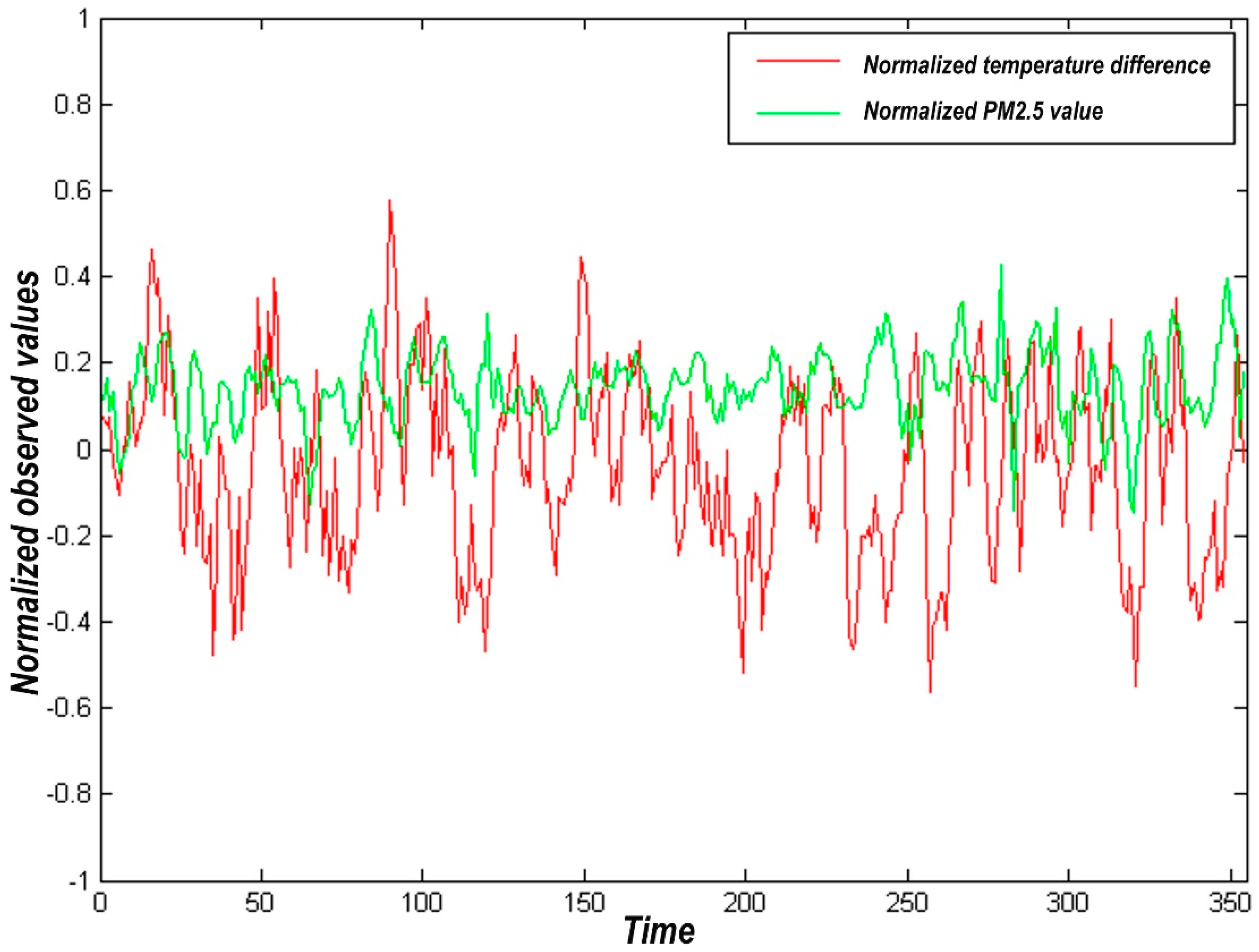
Abstract
:1. Introduction
2. Data and Study Area
3. Methods
3.1. Spatial Autocorrelation
Global Spatial Autocorrelation
3.2. Grey Relational Analysis Model
4. Results
4.1. Correlation Analysis of PM2.5 and Aerodynamic Factors
4.1.1. Temperature Difference
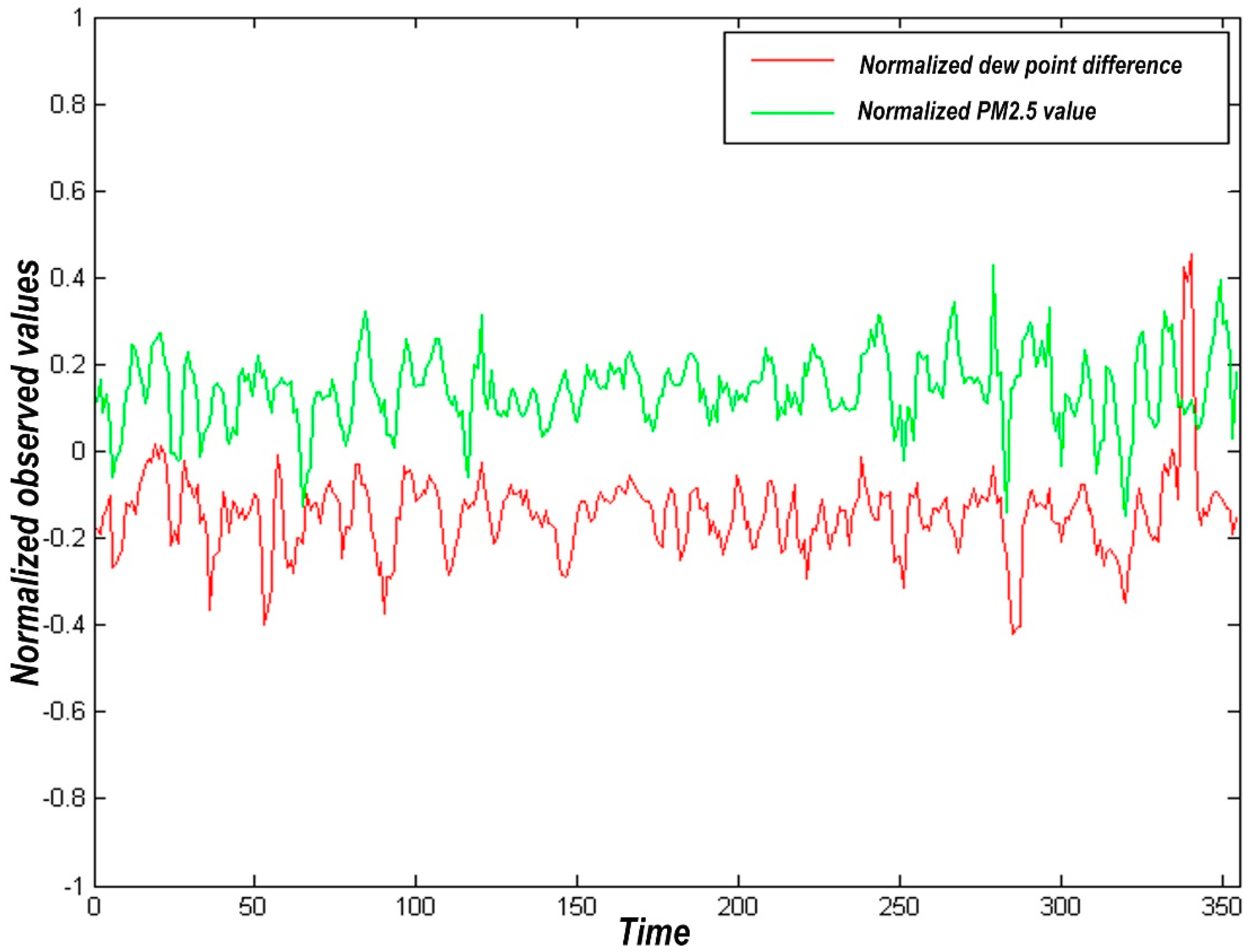
4.1.2. Dew Point Difference
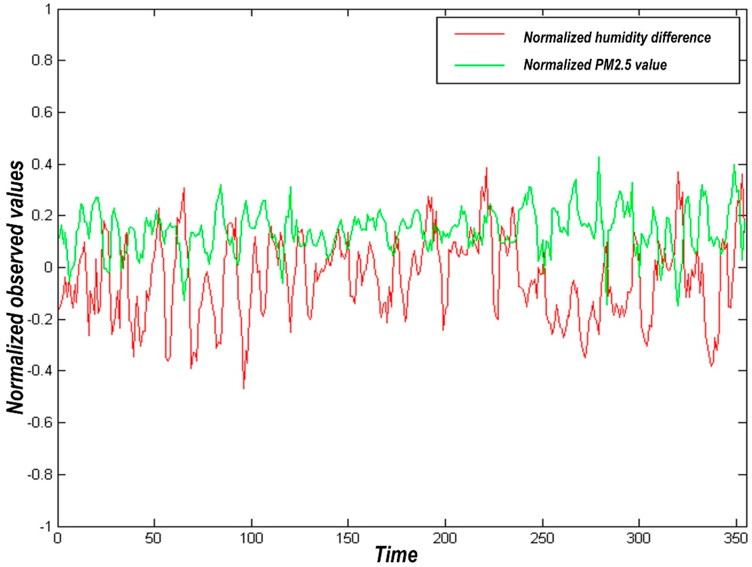
4.1.3. Humidity Difference
- Humidity influences the diffusion and migration of PM2.5 and the composition of PM2.5.
- When the composition of PM2.5 is different, humidity has different effects on its concentration. Secondary particles such as nitrate and sulfate are more likely to be generated when humidity is high. Some studies have pointed out that the culprit for haze weather is such secondary particles.
- When the atmospheric state is relatively stable, water vapor in the high-humidity atmosphere is adsorbed on the suspended PM2.5, causing haze weather.
- The influence of humidity on PM2.5 concentration exists complex and different mechanisms in different threshold ranges.
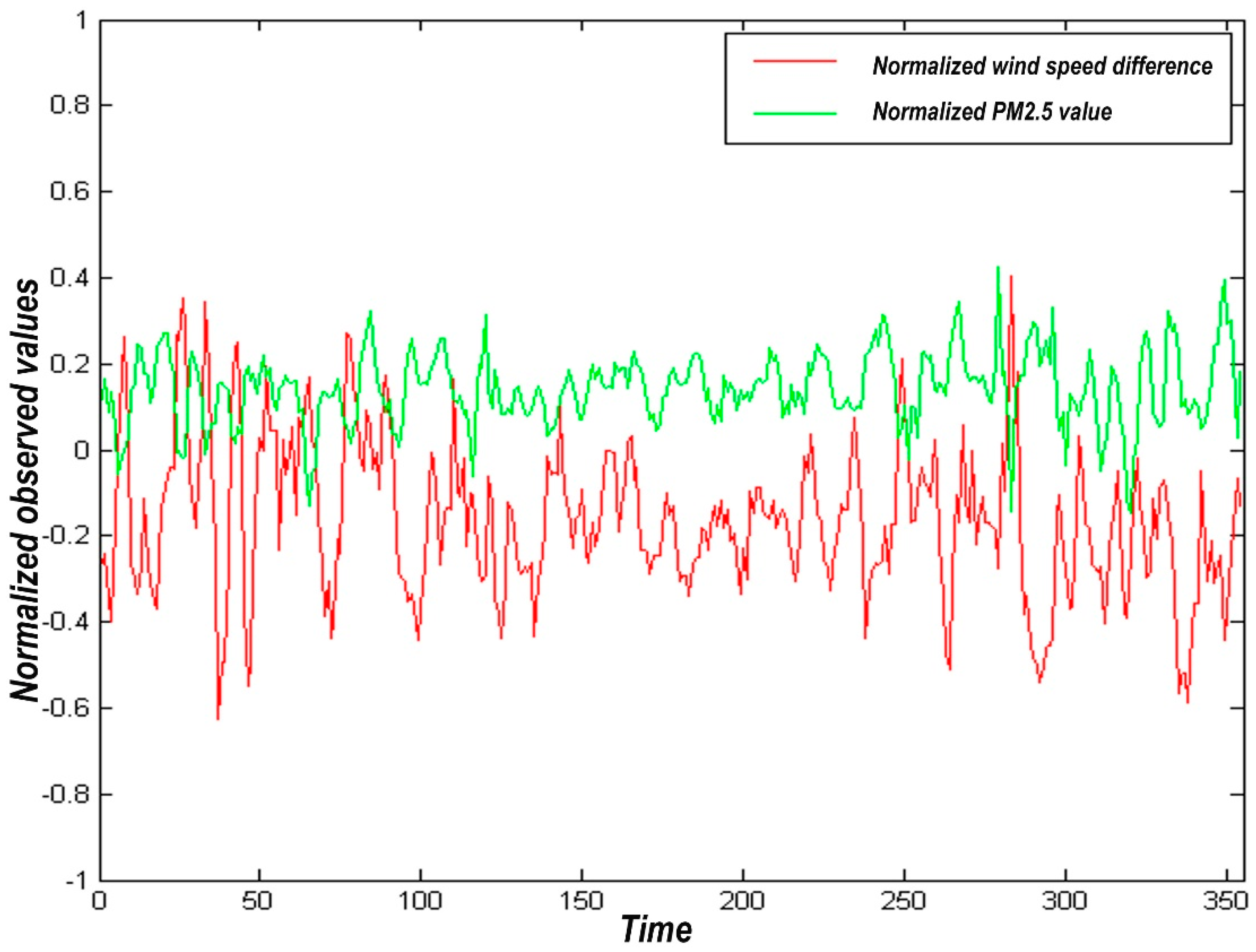
4.1.4. Wind Speed Difference
4.2. Grey Correlation Analysis of PM2.5 and Aerodynamic Factors
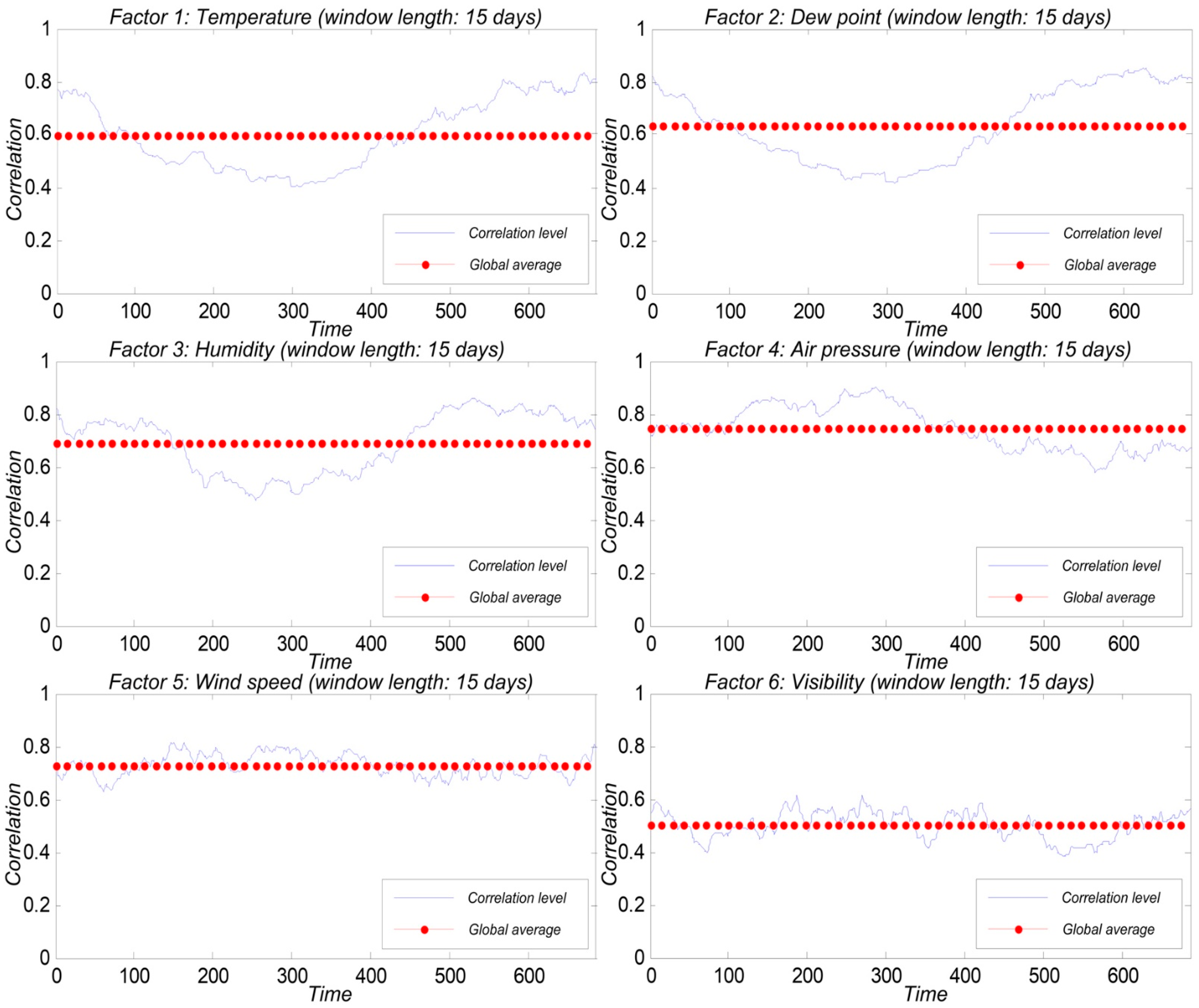
4.2.1. Grey Correlation Analysis Based on Time Window
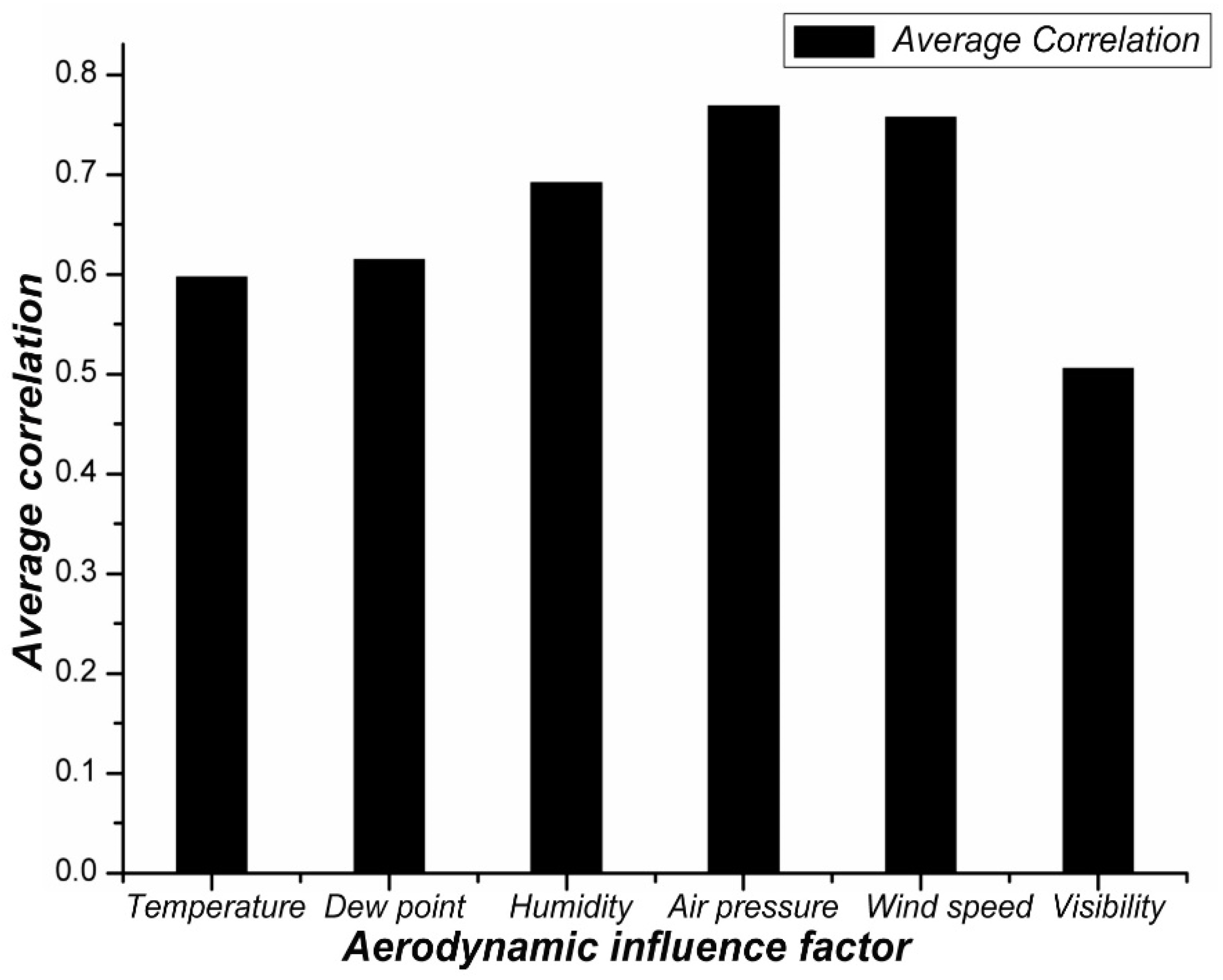
4.2.2. Average Grey Correlation
5. Discussion
- The research mainly focuses on PM2.5, but NOx is also an essential part of the haze pollution components. As accurate data cannot be obtained in this paper, the analysis of this influence factor is abandoned. However, with the escalation of environmental monitoring in my country, we will continue participating in NOx research [37].
- This article analyzes the impact of human activities on smog pollution. However, there is a lack of in-depth discussion on developing the social economy rationally, and further research is needed in future research [41].
6. Conclusions
- (1)
- The requirements for the amount of data are broad. The gray relational analysis can use fewer data to obtain relevant results. The minimum amount of data that can be calculated is 4, which can be applied to irregular random data.
- (2)
- Traditional methods such as analysis of variance have requirements for the sequence itself. For example, the sample sequence must have probability distribution characteristics. There is no correlation between the sequences, which significantly limits the range of sequences that can be analyzed.
- (3)
- Grey relational analysis is relatively concise in modeling, and the amount of calculation is small.
- (4)
- Grey relational analysis has high accuracy and can be highly consistent with the results of qualitative analysis. That is, the quantitative results will fit the objective laws of the system and the interrelationships between elements.
Author Contributions
Funding
Institutional Review Board Statement
Informed Consent Statement
Data Availability Statement
Conflicts of Interest
References
- Li, X.; Yin, L.; Yao, L.; Yu, W.; She, X.; Wei, W. Seismic spatiotemporal characteristics in the Alpide Himalayan Seismic Belt. Earth Sci. Inform. 2020, 13, 883–892. [Google Scholar] [CrossRef]
- Yin, L.; Li, X.; Zheng, W.; Yin, Z.; Song, L.; Ge, L.; Zeng, Q. Fractal dimension analysis for seismicity spatial and temporal distribution in the circum-Pacific seismic belt. J. Earth Syst. Sci. 2019, 128, 22. [Google Scholar] [CrossRef] [Green Version]
- Chen, X.; Yin, L.; Fan, Y.; Song, L.; Ji, T.; Liu, Y.; Tian, J.; Zheng, W. Temporal evolution characteristics of PM2. 5 concentration based on continuous wavelet transform. Sci. Total Environ. 2020, 699, 134244. [Google Scholar] [CrossRef]
- Zheng, W.; Li, X.; Yin, L.; Wang, Y. Spatiotemporal heterogeneity of urban air pollution in China based on spatial analysis. Rend. Lincei 2016, 27, 351–356. [Google Scholar] [CrossRef]
- Han, Y.; Bandowe, B.A.M.; Schneider, T.; Pongpiachan, S.; Ho, S.S.H.; Wei, C.; Wang, Q.; Xing, L.; Wilcke, W. A 150-year record of black carbon (soot and char) and polycyclic aromatic compounds deposition in Lake Phayao, north Thailand. Environ. Pollut. 2021, 269, 116148. [Google Scholar] [CrossRef]
- Guo, B.; Wang, Y.; Zhang, X.; Che, H.; Zhong, J.; Chu, Y.; Cheng, L. Temporal and spatial variations of haze and fog and the characteristics of PM2. 5 during heavy pollution episodes in China from 2013 to 2018. Atmos. Pollut. Res. 2020, 11, 1847–1856. [Google Scholar] [CrossRef]
- Li, Q.; Xia, M.; Guo, X.; Shi, Y.; Guan, R.; Liu, Q.; Cai, Y.; Lu, H. Spatial characteristics and influencing factors of risk perception of haze in China: The case study of publishing online comments about haze news on Sina. Sci. Total Environ. 2021, 785, 147236. [Google Scholar] [CrossRef]
- Tang, Y.; Liu, S.; Deng, Y.; Zhang, Y.; Yin, L.; Zheng, W. Construction of force haptic reappearance system based on Geomagic Touch haptic device. Comput. Methods Programs Biomed. 2020, 190, 105344. [Google Scholar] [CrossRef]
- Yin, L.; Wang, L.; Huang, W.; Liu, S.; Yang, B.; Zheng, W. Spatiotemporal Analysis of Haze in Beijing Based on the Multi-Convolution Model. Atmosphere 2021, 12, 1408. [Google Scholar] [CrossRef]
- Zhang, Z.; Tian, J.; Huang, W.; Yin, L.; Zheng, W.; Liu, S. A Haze Prediction Method Based on One-Dimensional Convolutional Neural Network. Atmosphere 2021, 12, 1327. [Google Scholar] [CrossRef]
- Wang, X.; Yin, C.; Shao, C. Relationships among haze pollution, commuting behavior and life satisfaction: A quasi-longitudinal analysis. Transp. Res. Part D Transp. Environ. 2021, 92, 102723. [Google Scholar] [CrossRef]
- Liu, S.; Wang, L.; Liu, H.; Su, H.; Li, X.; Zheng, W. Deriving bathymetry from optical images with a localized neural network algorithm. IEEE Trans. Geosci. Remote Sens. 2018, 56, 5334–5342. [Google Scholar] [CrossRef]
- Tang, Y.; Liu, S.; Deng, Y.; Zhang, Y.; Yin, L.; Zheng, W. An improved method for soft tissue modeling. Biomed. Signal. Process. Control 2021, 65, 102367. [Google Scholar] [CrossRef]
- Ma, Z.; Zheng, W.; Chen, X.; Yin, L. Joint embedding VQA model based on dynamic word vector. PeerJ Comput. Sci. 2021, 7, e353. [Google Scholar] [CrossRef]
- Li, Y.; Zheng, W.; Liu, X.; Mou, Y.; Yin, L.; Yang, B. Research and improvement of feature detection algorithm based on FAST. Rend. Lincei Sci. Fis. E Nat. 2021, 1–15. [Google Scholar] [CrossRef]
- Deng, Y.; Tang, Y.; Yang, B.; Zheng, W.; Liu, S.; Liu, C. A Review of Bilateral Teleoperation Control Strategies with Soft Environment. In Proceedings of the 2021 6th IEEE International Conference on Advanced Robotics and Mechatronics (ICARM), Chongqing, China, 3–5 July 2021; pp. 459–464. [Google Scholar]
- Wu, X.; Liu, Z.; Yin, L.; Zheng, W.; Song, L.; Tian, J.; Yang, B.; Liu, S. A Haze Prediction Model in Chengdu Based on LSTM. Atmosphere 2021, 12, 1479. [Google Scholar] [CrossRef]
- Zheng, W.; Liu, X.; Yin, L. Sentence Representation Method Based on Multi-Layer Semantic Network. Appl. Sci. 2021, 11, 1316. [Google Scholar] [CrossRef]
- Zheng, W.; Liu, X.; Ni, X.; Yin, L.; Yang, B. Improving Visual Reasoning Through Semantic Representation. IEEE Access 2021, 9, 91476–91486. [Google Scholar] [CrossRef]
- Zheng, W.; Yin, L.; Chen, X.; Ma, Z.; Liu, S.; Yang, B. Knowledge base graph embedding module design for Visual question answering model. Pattern Recognit. 2021, 120, 108153. [Google Scholar] [CrossRef]
- Zheng, W.; Liu, X.; Yin, L. Research on image classification method based on improved multi-scale relational network. PeerJ Comput. Sci. 2021, 7, e613. [Google Scholar] [CrossRef]
- Li, M.; Hu, M.; Guo, Q.; Tan, T.; Du, B.; Huang, X.; He, L.; Guo, S.; Wang, W.; Fan, Y. Seasonal source apportionment of PM2. 5 in Ningbo, a coastal city in southeast China. Aerosol Air Qual. Res. 2018, 18, 2741–2752. [Google Scholar] [CrossRef]
- Lu, M.; Tang, X.; Feng, Y.; Wang, Z.; Chen, X.; Kong, L.; Ji, D.; Liu, Z.; Liu, K.; Wu, H. Nonlinear response of SIA to emission changes and chemical processes over eastern and central China during a heavy haze month. Sci. Total Environ. 2021, 788, 147747. [Google Scholar] [CrossRef]
- Yao, W.; Zheng, Z.; Zhao, J.; Wang, X.; Wang, Y.; Li, X.; Fu, J. The factor analysis of fog and haze under the coupling of multiple factors—Taking four Chinese cities as an example. Energy Policy 2020, 137, 111138. [Google Scholar] [CrossRef]
- Gan, T.; Yang, H.; Liang, W.; Liao, X. Do economic development and population agglomeration inevitably aggravate haze pollution in China? New evidence from spatial econometric analysis. Environ. Sci. Pollut. Res. 2021, 28, 5063–5079. [Google Scholar] [CrossRef]
- Wu, Q.; Jiang, Y.; Shi, T.; Miao, J.; Qi, B.; Du, R.; Luo, Y.; Chi, X. Quantifying Analysis of the Impact of Haze on Photovoltaic Power Generation. IEEE Access 2020, 8, 215977–215986. [Google Scholar] [CrossRef]
- Zheng, W.; Li, X.; Xie, J.; Yin, L.; Wang, Y. Impact of human activities on haze in Beijing based on grey relational analysis. Rend. Lincei 2015, 26, 187–192. [Google Scholar] [CrossRef]
- Li, X.; Zheng, W.; Yin, L.; Yin, Z.; Song, L.; Tian, X. Influence of social-economic activities on air pollutants in Beijing, China. Open Geosci. 2017, 9, 314–321. [Google Scholar] [CrossRef] [Green Version]
- Tang, L.; Yu, H.; Ding, A.; Zhang, Y.; Qin, W.; Wang, Z.; Chen, W.; Hua, Y.; Yang, X. Regional contribution to PM1 pollution during winter haze in Yangtze River Delta, China. Sci. Total Environ. 2016, 541, 161–166. [Google Scholar] [CrossRef]
- Zhang, B.; Zhe, H.; Wang, J.; Wu, H. Study on the total amount control of atmospheric environment based on CALPUFF atmospheric diffusion model. North. Environ. 2011, 6, 95–96. [Google Scholar]
- Cai, H.-Y.; Xu, Y.-Z.; Sun, W.-Y. Regional differences and convergence of haze pollution intensity distribution in China—The empirical analysis based on provincial panel data. J. Shanxi Univ. Financ. Econ. 2017, 39, 1–14. [Google Scholar]
- He, J.; Zhao, M.; Zhang, B.; Wang, P.; Zhang, D.; Wang, M.; Liu, B.; Li, N.; Yu, K.; Zhang, Y. The impact of steel emissions on air quality and pollution control strategy in Caofeidian, North China. Atmos. Pollut. Res. 2020, 11, 1238–1247. [Google Scholar] [CrossRef]
- Di Nicolantonio, W.; Cacciari, A.; Petritoli, A.; Carnevale, C.; Pisoni, E.; Volta, M.; Stocchi, P.; Curci, G.; Bolzacchini, E.; Ferrero, L. MODIS and OMI satellite observations supporting air quality monitoring. Radiat. Prot. Dosim. 2009, 137, 280–287. [Google Scholar] [CrossRef] [PubMed]
- Sorek-Hamer, M.; Chatfield, R.; Liu, Y. Strategies for using satellite-based products in modeling PM2. 5 and short-term pollution episodes. Environ. Int. 2020, 144, 106057. [Google Scholar] [CrossRef] [PubMed]
- Mishra, R.K.; Agarwal, A.; Shukla, A. Predicting Ground Level PM2.5 Concentration over Delhi Using Landsat 8 Satellite Data. Int. J. Remote Sens. 2021, 42, 827–838. [Google Scholar] [CrossRef]
- Zhao, X.; Huang, X.; Liu, Y. Spatial autocorrelation analysis of Chinese inter-provincial industrial chemical oxygen demand discharge. Int. J. Environ. Res. Public Health 2012, 9, 2031–2044. [Google Scholar] [CrossRef] [Green Version]
- Tsai, V.C.; Moschetti, M.P. An explicit relationship between time-domain noise correlation and spatial autocorrelation (SPAC) results. Geophys. J. Int. 2010, 182, 454–460. [Google Scholar] [CrossRef] [Green Version]
- Wang, Q.; Liu, J.; Zhu, X.; Liu, J.; Liu, Z. The experiment study of frost heave characteristics and gray correlation analysis of graded crushed rock. Cold Reg. Sci. Technol. 2016, 126, 44–50. [Google Scholar] [CrossRef]
- Ren, C.; Huang, X.; Wang, Z.; Sun, P.; Chi, X.; Ma, Y.; Zhou, D.; Huang, J.; Xie, Y.; Gao, J. Nonlinear response of nitrate to NOx reduction in China during the COVID-19 pandemic. Atmos. Environ. 2021, 264, 118715. [Google Scholar] [CrossRef]
- Shi, X.; Liu, Y. Sample Contribution Pattern Based Big Data Mining Optimization Algorithms. IEEE Access 2021, 9, 32734–32746. [Google Scholar] [CrossRef]
- Gan, T.; Yang, H.; Liang, W. How do urban haze pollution and economic development affect each other? Empirical evidence from 287 Chinese cities during 2000–2016. Sustain. Cities Soc. 2021, 65, 102642. [Google Scholar] [CrossRef]


Publisher’s Note: MDPI stays neutral with regard to jurisdictional claims in published maps and institutional affiliations. |
© 2021 by the authors. Licensee MDPI, Basel, Switzerland. This article is an open access article distributed under the terms and conditions of the Creative Commons Attribution (CC BY) license (https://creativecommons.org/licenses/by/4.0/).
Share and Cite
Xu, J.; Liu, Z.; Yin, L.; Liu, Y.; Tian, J.; Gu, Y.; Zheng, W.; Yang, B.; Liu, S. Grey Correlation Analysis of Haze Impact Factor PM2.5. Atmosphere 2021, 12, 1513. https://doi.org/10.3390/atmos12111513
Xu J, Liu Z, Yin L, Liu Y, Tian J, Gu Y, Zheng W, Yang B, Liu S. Grey Correlation Analysis of Haze Impact Factor PM2.5. Atmosphere. 2021; 12(11):1513. https://doi.org/10.3390/atmos12111513
Chicago/Turabian StyleXu, Jiayi, Zhixin Liu, Lirong Yin, Yan Liu, Jiawei Tian, Yang Gu, Wenfeng Zheng, Bo Yang, and Shan Liu. 2021. "Grey Correlation Analysis of Haze Impact Factor PM2.5" Atmosphere 12, no. 11: 1513. https://doi.org/10.3390/atmos12111513