
Parameterization of Sea Surface Drag Coefficient for All Wind Regimes Using 11 Aircraft Eddy-Covariance Measurement Databases


Abstract
:1. Introduction
2. Database
- (1)
- The Long-EZ aircraft of the National Oceanic and Atmospheric Administration (NOAA) during the four experiments: (1) the pilot program of the Coupled Boundary Layers and Air Sea Transfer experiment (CBLAST Weak Wind) conducted during July–August 2001 over the Atlantic Ocean south of Martha’s Vineyard Island, MA [15]; (2) the Shoaling Waves experiment (SHOWEX) over the Atlantic east of the Outer Banks near Duck, NC during November and December 1999 [16]; (3) the SHOWEX pilot study in November 1997; and (4) the SHOWEX pilot study in March 1999.
- (2)
- The Naval Postgraduate School’s Center for Interdisciplinary Remotely-Piloted Aircraft Studies (CIRPAS) Twin Otter aircraft in five experiments: (1) outside Monterey Bay off the coast of California during the Cloud-Aerosol Research in the Marine Atmosphere IV experiment (CARMAIV) in August 2007; (2) outside Monterey Bay (Monterey) during April 2008 [17]; (3) the Rough Evaporation Duct experiment (RED) during August–September of 2001 to the east (windward side) of Oahu in the Hawaiian Islands [18]; (4) the Marine Atmospheric Boundary Layer Energy Budget (MABLEB) experiment during April 2007; and (5) the Physics Of Stratocumulus Top during July–August 2008 (POST).
- (3)
- The C-130 Hercules aircraft of the National Center for Atmospheric Research (NCAR) in the Gulf of Tehuantepec Experiment (GOTEX) in February 2004 on the Pacific coast of the Isthmus of Tehuantepec, Mexico [19], and the data collected by the NCAR Electra aircraft in TOGA COARE during November 1992 to February 1993 in the Pacific warm pool [20].
3. Results
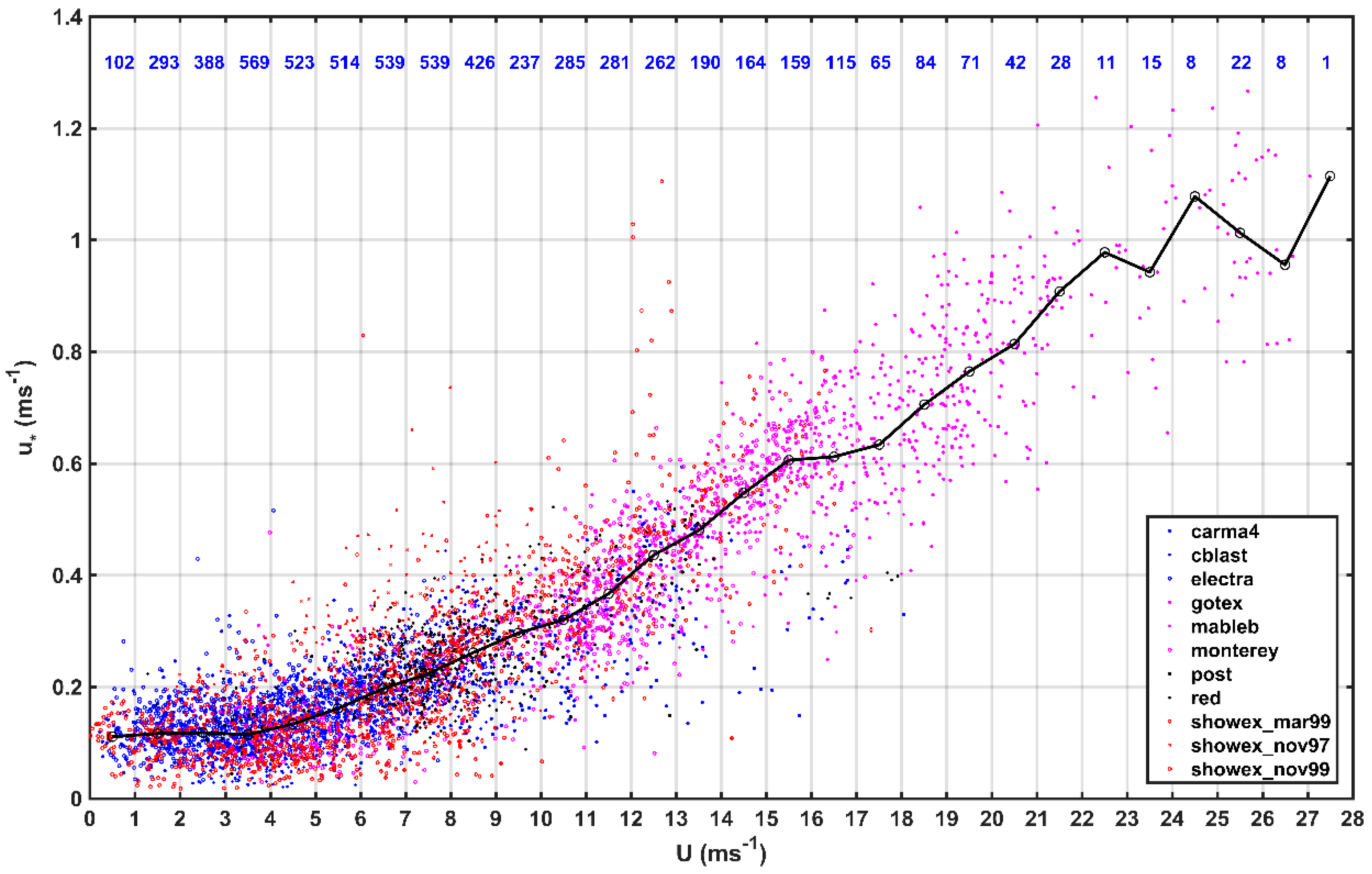
3.1. Variation of Friction Velocity () against Wind Speed
3.2. Parameterizations of Turbulent Drag Coefficient ()
3.3. Parameterizations of Turbulent Heat Transfer Coefficient () and Water Vapor Transfer Coefficient ()
4. Conclusions
Author Contributions
Funding
Institutional Review Board Statement
Informed Consent Statement
Data Availability Statement
Acknowledgments
Conflicts of Interest
References
- Garratt, J.R. The Atmospheric Boundary Layer; Cambridge University Press: New York, NY, USA, 1992; p. 316. [Google Scholar]
- Nosov, V.V.; Lukin, V.P.; Nosov, E.V.; Torgaev, A.V. Turbulence Scales of the Monin-Obukhov Similarity Theory in the Anisotropic Mountain Boundary Layer. Russ. Phys. J. 2020, 63, 244–249. [Google Scholar] [CrossRef]
- Shikhovtsev, A.; Kovadlo, P.; Lukin, V. Temporal variations of the turbulence profiles at the Sayan solar observatory site. Atmosphere 2019, 10, 499. [Google Scholar] [CrossRef] [Green Version]
- Deskos, G.; Carre, A.; Palacios, R. Assessment of low-altitude atmospheric turbulence models for aircraft aeroelasticity. J. Fluids Struct. 2020, 95, 102981. [Google Scholar] [CrossRef] [Green Version]
- Gao, Z.; Peng, W.; Gao, C.Y.; Li, Y. Parabolic dependence of the drag coefficient on wind speed from aircraft eddy-covariance measurements over the tropical Eastern Pacific. Sci. Rep. 2020, 10, 1805. [Google Scholar] [CrossRef] [PubMed]
- Alamaro, M.; Emanuel, K.A.; McGillis, W.R. Experimental investigation of air-sea transfer of momentum and enthalpy at high wind speed. In Preprints, Proceedings of the 25th Conference on Hurricane and Tropical Meteorology, San Diego, CA, USA, 28 April–3 May 2002; American Meteorological Society: San Diego, CA, USA, 2002; pp. 667–668. [Google Scholar]
- Powell, M.D.; Vickery, P.J.; Reinhold, T.A. Reduced drag coefficient for high wind speeds in tropical cyclones. Nature 2003, 422, 279–283. [Google Scholar] [CrossRef] [PubMed]
- Donelan, M.A.; Haus, B.K.; Reul, N.; Plant, W.J.; Stiassnie, M.; Graber, H.C.; Brown, O.B.; Saltzman, E.S. On the limiting aerodynamic roughness of the ocean in very strong winds. Geophys. Res. Lett. 2004, 31, L18306. [Google Scholar] [CrossRef] [Green Version]
- Makin, V.K. A note on drag of the sea surface at Hurricane winds. Bound. Layer Meteorol. 2005, 115, 169–176. [Google Scholar] [CrossRef]
- Black, P.G.; Dasaro, E.A.; Drennan, W.M.; French, J.R.; Niiler, P.P.; Sanford, T.B.; Terrill, E.; Walsh, E.J.; Zhang, J.A. Air–Sea Exchange in Hurricanes: Synthesis of Observations from the Coupled Boundary Layer Air-Sea Transfer Experiment. Bull. Am. Meteorol. Soc. 2007, 88, 357–374. [Google Scholar] [CrossRef] [Green Version]
- Troitskaya, Y.I.; Sergeev, D.A.; Kandaurov, A.A.; Baidakov, G.A.; Vdovin, M.A.; Kazakov, V.I. Laboratory and theoretical modeling of air-sea momentum transfer under severe wind conditions. J. Geophys. Res. 2012, 117, C00J21. [Google Scholar] [CrossRef]
- Soloviev, A.V.; Lukas, R.; Donelan, M.A.; Haus, B.K.; Ginis, I. The air-sea interface and surface stress under tropical cyclones. Sci. Rep. 2014, 4, 5306. [Google Scholar] [CrossRef]
- Donelan, M.A. On the decrease of the oceanic drag coefficient in high winds. J. Geophys. Res. Ocean. 2018, 123, 1485–1501. [Google Scholar] [CrossRef]
- Vickers, D.; Mahrt, L.; Andreas, E.L. Estimates of the 10-m neutral sea surface drag coefficient from aircraft eddy-covariance measurements. J. Phys. Oceanogr. 2013, 43, 301–310. [Google Scholar] [CrossRef]
- Edson, J.B.; Crawford, T.; Crescenti, J.; Farrar, T.; Frew, N.; Gerbi, G.; Helmis, C.; Hristov, T.; Khelif, D.; Jessup, A.; et al. The coupled boundary layers and air-sea transfer experiment in low winds. Bull. Am. Meteorol. Soc. 2007, 88, 341–356. [Google Scholar] [CrossRef]
- Sun, J.; Vandemark, D.; Mahrt, L.; Vickers, D.; Crawford, T.; Vogel, C. Momentum transfer over the coastal zone. J. Geophys. Res. 2001, 106, 12437–12448. [Google Scholar] [CrossRef] [Green Version]
- Khelif, D.; Burns, S.P.; Friehe, C.A. Improved wind measurements on research aircraft. J. Atmos. Ocean. Technol. 1999, 16, 860–875. [Google Scholar] [CrossRef]
- Anderson, K.; Brooks, B.; Caffrey, P.; Clarke, A.; Cohen, L.; Crahan, K.; Davidson, K.; De Jong, A.; De Leeuw, G.; Dion, D.; et al. The RED Experiment: An assessment of boundary layer effects in a trade winds regime on microwave and infrared propagation over the sea. Bull. Am. Meteorol. Soc. 2014, 85, 1355–1366. [Google Scholar] [CrossRef]
- Raga, G.; Abarca, S. On the parameterization of turbulent fluxes over the tropical eastern Pacific. Amer. Chem. Phys. 2007, 7, 635–643. [Google Scholar] [CrossRef] [Green Version]
- Vickers, D.; Esbensen, S.K. Subgrid surface fluxes in fair weather conditions during TOGA COARE: Observational estimates and parameterization. Mon. Weather Rev. 1998, 126, 620–633. [Google Scholar] [CrossRef]
- Mahrt, L.; Scott, M.; Tihomir, H.; James, E. On Estimating the Surface Wind Stress over the Sea. J. Phys. Oceanogr. 2018, 48, 1533–1541. [Google Scholar] [CrossRef]


| Reference | Saturated Wind Speed (ms−1) | Comments |
|---|---|---|
| Alamaro et al. [6] | 35 | Laboratory annular wind wave tank. |
| Powell et al. [7] | 33 | Global Positioning System sonde observations in tropical cyclone environments. |
| Donelan et al. [8] | 33 | Laboratory extreme wind experiments. |
| Makin [9] | 30–40 | Solving the turbulent kinetic energy balance equation for airflow under the limited saturation (by suspended sea-spray droplets) regime. |
| Black et al. [10] | 23 | The Coupled Boundary Layer Air-Sea Transfer (CBLAST) Experiment. |
| Troitskaya et al. [11] | 25 | Theoretically and laboratory experiment. |
| Soloviev et al. [12] | 30 | The unified wave-form and two-phase parameterization model. |
| Donelan [13] | 30 | Laboratory extreme wind experiments. |
| Gao et al. [5] | 22–23 | Mathematical regression for aircraft eddy-covariance measurements over the tropical Eastern Pacific. |
Publisher’s Note: MDPI stays neutral with regard to jurisdictional claims in published maps and institutional affiliations. |
© 2021 by the authors. Licensee MDPI, Basel, Switzerland. This article is an open access article distributed under the terms and conditions of the Creative Commons Attribution (CC BY) license (https://creativecommons.org/licenses/by/4.0/).
Share and Cite
Gao, Z.; Zhou, S.; Zhang, J.; Zeng, Z.; Bi, X. Parameterization of Sea Surface Drag Coefficient for All Wind Regimes Using 11 Aircraft Eddy-Covariance Measurement Databases. Atmosphere 2021, 12, 1485. https://doi.org/10.3390/atmos12111485
Gao Z, Zhou S, Zhang J, Zeng Z, Bi X. Parameterization of Sea Surface Drag Coefficient for All Wind Regimes Using 11 Aircraft Eddy-Covariance Measurement Databases. Atmosphere. 2021; 12(11):1485. https://doi.org/10.3390/atmos12111485
Chicago/Turabian StyleGao, Zhiqiu, Shaohui Zhou, Jianbin Zhang, Zhihua Zeng, and Xueyan Bi. 2021. "Parameterization of Sea Surface Drag Coefficient for All Wind Regimes Using 11 Aircraft Eddy-Covariance Measurement Databases" Atmosphere 12, no. 11: 1485. https://doi.org/10.3390/atmos12111485