Chemical Characterization, Source, and SOA Production of Intermediate Volatile Organic Compounds during Haze Episodes in North China

Abstract

The growth of secondary organic aerosols (SOA) is a vital cause of the outbreaks of winter haze in North China. Intermediate volatile organic compounds (IVOCs) are important precursors of SOA. Therefore, the chemical characteristics, source, and SOA production of IVOCs during haze episodes have attracted much attention. Hourly time resolution IVOC samples during two haze episodes collected in Hebei Province in North China were analyzed in this study. Results showed that: (1) the concentration of IVOCs measured was within the range of 11.3~85.1 μg·cm⁻³ during haze episodes, with normal alkanes (n-alkanes), polycyclic aromatic hydrocarbons (PAHs), branched alkanes (b-alkanes), and the residue unresolved complex mixture (R-UCM) accounting for 8.6 ± 2.3%, 6.8 ± 2.2%, 24.1 ± 3.8%, and 60.5 ± 6.5% of IVOCs, respectively. NC₁₂-nC₁₅ in n-alkanes, naphthalene and its alkyl substitutes in PAHs, b-alkanes in B₁₂–B₁₆ bins, and R-UCM in B₁₂–B₁₆ bins are the main components, accounting for 87.0 ± 0.2%, 87.6 ± 2.9%, 85.9 ± 5.4%, 74.0 ± 8.3%, respectively. (2) Based on the component characteristics of IVOCs and the ratios of n-alkanes/b-alkanes in emission sources and the hourly variation of IVOCs during haze episodes, coal combustion (CC), biomass burning (BB), gasoline vehicles (GV), and diesel vehicles (DV)were identified as important emission sources of IVOCs in Hebei Province. (3) During haze episodes, temporal variation of the estimated SOA production based on different methods (such as IVOCs concentration, OC/EC_min tracer, and the PMF model) were similar; however, the absolute values were different. This difference may be due to the transformation of IVOCs to SOA affected by various factors such as SOA production from different IVOC components, meteorological conditions, atmospheric oxidation, etc.

1. Introduction

The increase in secondary organic aerosols (SOA) is a vital cause of the outbreaks of winter haze in North China. The haze episodes in Beijing, Tianjin, Shijiazhuang, and Chengde showed that organic matter (OM) increased and became the dominant component of PM_2.5 [1]. Liu et al. [2] showed that SOA to total carbon is 54% in Beijing and 46% in Tianjin. There are still great uncertainties in the formation mechanism and sources of SOA. In recent years, simulated SOA production based on precursors of VOCs (usually C₂–C₈ hydrocarbons, such as benzene, toluene, xylene, isoprene, monoterpenes, etc.) has been significantly underestimated [3]. The observed SOA concentration cannot be fully explained by the known mechanisms of the formation of SOA from VOCs [4]. Intermediate volatile organic compounds (IVOCs) are another major precursor of SOA. A study by Couvidat et al. [5] showed that without adding IVOCs to the model, the yields of SOA simulated by the model were lower than the observed value. Presto et al. [6] present evidence for the formation of highly oxygenated SOA from the photooxidation of nC₁₇, which was used as a proxy for IVOCs emissions. Huang et al. [7] estimated that the contribution rate of naphthalene and its alkyl substitutes to SOA was as high as 14.9% during the winter haze in Beijing, which is equivalent to that of monocyclic aromatic hydrocarbons. Chan et al. [8] and Kautzman et al. [3] showed that the oxidation of naphthalene under high NOx conditions produced semi-volatile SOA with a yield of 73%, and oxidation of naphthalene under low NOx conditions produced substantially non-volatile SOA with a yield of 13–30% [9]. Zhao et al. [10] showed that IVOCs contribute 46% to average OA concentrations in Eastern China and 58% to average SOA concentrations in the CMAQ/2D-VBS model simulation. The researcher added IVOCs to the model to evaluate the yield of SOA and showed that gas-phase C₆–C₁₉ alkanes and low-ring PAHs are expected to explain 20–30% of the artificially formed SOA when IVOC or semi-volatile organic compounds (SVOC) are added to the model [11]. Woody et al. [12] found that the simulated SOA was closer to the measured value after adding IVOCs to the model, which can correct the estimated effect of the traditional model on SOA production.

In recent years, researchers have paid increasing attention to IVOCs. Most of the research has focused on the chemical characterization of IVOC in various source emissions such as biomass burning (BB) and coal combustion (CC) [13,14], gasoline vehicles (GV) [15], diesel vehicles (DV) [16,17], heavy fuel oil vessels (HFOVs) [18], non-road construction machinery (NRCM) [19], and aircraft [20]. Additionally, some studies have investigated concentration levels and chemical characterization of IVOCs in an ambient atmosphere [21,22]. For example, Wang et al. [21] reported the concentration and composition of IVOCs in the ambient atmosphere of Yangshan Port in Shanghai. Furthermore, Li et al. [22] studied the seasonal variation of concentration and chemical characterization of IVOCs in the ambient atmosphere of Shanghai. However, knowledge about the chemical characterization, emission sources, and SOA production of IVOCs during haze episodes, especially in the heavily polluted area in China, is still very limited. In this study, we collected IVOCs samples with an hourly time resolution during two haze episodes in winter in Wangdu County, Hebei Province, a city in North China with a frequent occurrence of winter haze episodes. The objectives of this study include (1) to investigate the chemical characterization of IVOCs in a heavily polluted ambient atmosphere; (2) to explore the sources of IVOCs and associated variation during haze episodes; and (3) to assess IVOC contribution to SOA production, to provide theoretical support for mitigating the outbreaks of haze episodes.

2. Materials and Methods

2.1. Sampling Collection

Hourly time resolution PM_2.5 and IVOCs samples were collected at a rural environmental monitoring station of the Institute of Environmental Ecology, Chinese Academy of Sciences, which was located in Wangdu County, Hebei Province, in North China (Figure S1) during two haze episodes that occurred during 22–30 December 2019. PM_2.5 samples were collected on pre-baked quartz filters by a sampler (TE-6070, TISCH, 1.13 m³·min⁻¹). IVOCs samples were collected by a portable 8-channel remote-controlled automatic sampler (Shanghai Xinxiao Environmental Technology Co., Ltd., Shanghai, China). The sampling channel was switched each hour to obtain hourly resolution IVOCs samples. Briefly, IVOCs were sampled at a flow rate of 0.5 L·min⁻¹ through the sampling tube with a Tenax TA sorbent. After sampling, the sample filters and tubes were immediately sealed and stored in a refrigerator at −20 °C until analysis. The data of meteorological parameters such as temperature (T), humidity (RH) and wind speed (WS), and air pollutants (e.g., PM_2.5, PM₁₀, SO₂, NO_x, CO, O₃) were obtained from the Environmental Monitoring Station in Wangdu County, which was about 10 km away from the sampling site.

2.2. Chemical Analysis

IVOCs samples were analyzed by thermal desorption-gas chromatography-mass spectrometry (TD-GC/MS) method (TD: Sciences Optic-4, Shimadzu, GC/MS: Thermo Trace 1300/ISQ 7000, Thermo Fisher Scientific, Waltham, MA, USA). A detailed description of the analysis protocols and quantification methods for IVOCs can be found in previous studies [10,13,15]. Generally, four parts of IVOCs, including normal alkanes (n-alkanes, nC₁₂–nC₂₂), branched alkanes (b-alkanes), polycyclic aromatic hydrocarbons (PAHs), and residue unresolved complex mixture (R-UCM), were identified and quantified in this study. Among them, n-alkanes (nC₁₂–nC₂₂) and PAHs were qualitatively and quantitatively determined by standard products purchased from J&K Company, defined as speciated IVOCs. In total, nC₁₂–nC₂₂, eight parent PAHs (e.g., naphthalene (Nap), acenaphthylene (Acy), acenaphthene (Ace), fluorene (Flu), phenanthrene (Phe), anthracene (Ant), fluoranthene (Fluo), pyrene (Pyr)), and three methyl PAHs (e.g., 1-methylnaphthalene (1-Nap), 2-methylnaphthalene (2-Nap), and 2,6-dimethylnaphthalene (2,6-Nap)) were determined. According to the retention time of nC₁₂–nC₂₂, the total ion current (TIC) of IVOCs was divided into 11 bins (B_n, B₁₂–B₂₂). The IVOC concentration of each bin was calculated based on the TIC standard curve of the corresponding n-alkanes standards, and the mass sum of each bin was defined as the total IVOC concentration. The quantification of b-alkanes and R-UCM followed the methods by Zhao et al. [23] and Wang et al. [21]. Based on the premise that the m/z = 57 fragment signal comes from n-alkanes and b-alkanes, the mass of b-alkanes in each bin was quantified by the total mass of m/z = 57 minus the mass of n-alkanes in the corresponding bin. Finally, R-UCM mass was determined as the remaining mass of IVOCs after subtracting n-alkane, b-alkanes, and PAHs.

Meanwhile, the PM_2.5 composition was also analyzed. The concentrations of OC and EC were measured by a thermal-optical carbon analyzer (Sunset Laboratory Inc., Portland, OR, USA) with the IMPROVE A method [13]. Moreover, the filter sample was extracted with ultrasonic extraction and filtered, and then water-soluble ions in PM_2.5, including Na⁺, K⁺, Ca²⁺, Mg²⁺, Cl⁻, NO₃⁻, SO₄²⁻, and NH₄⁺, were analyzed by ion chromatography (IC, ICS 6000, Thermo Fisher Scientific, Waltham, MA, USA) based on the water extraction. The concentrations of inorganic elements (e.g., Na, Mg, Al, Fe, V, Cr, Mn, Ni, Cu, Zn, As, Cd, Pb) were measured by inductively coupled plasma and mass spectrometer (ICP-MS) [24]. Non-polar organic components, including alkanes (nC₃₁–nC₃₄) and 16 EPA-prioritized PAHs, were measured by GC/MS [25]. Polar organic components including levoglucosan (LEV), mannan (MAN), hexadecanoic acid (C₁₆A), and octadecanoic acid (C₁₈A) were determined by GC/MS after derivatization. The detailed determination method was described in the previous study [26]. Detailed information about the mass closure for the dataset of PM_2.5 is shown in Figure S2.

2.3. PMF Model

PMF 5.0 model was applied in this study to identify the source factors. Details of principles and information about the PMF model have been described in previous studies [27,28]. The uncertainty is half of the method detection limit (MDL) for data whose concentrations are below the MDL. When the concentration is slightly lower than or equal to the MDL, the uncertainty is calculated as 5/6 MDL. If the concentration is significantly greater than the MDL, it is calculated according to Equation (1):

$$\mathrm{Uncertainty}=\sqrt{{\left(\mathrm{error} \mathrm{factor}\times \mathrm{concentration}\right)}^2+{\left(0.5\times \mathrm{MDL}\right)}^2}$$

(1)

In addition, the error factor of these chemical components was chosen to be 20%. The detailed information about data preparation, factor determination (Figure S3), and error analysis (Table S1) of the PMF model was described in Text S1.

2.4. Estimation of SOA Production Based on Different Methods

In this study, SOA production was estimated by different methods. First, SOA production of IVOCs (defined as SOA_IVOCs) was estimated based on IVOC concentration following the method developed by Zhao et al. [23]. In this study, we also assumed that the hydrocarbon IVOCs (hydrocarbons) accounted for 60% of IVOCs, and oxygenated UCM accounted for the remaining 40% in the atmosphere of Wangdu Country, Hebei Province [23]. Hydrocarbon IVOCs include n-alkanes, PAHs, b-alkanes, and cyclic-alkanes. The detailed calculation methods for the cyclic-alkanes and oxygenated UCM are as follows:

$${\left[\mathrm{HC}\right]}_{\mathrm{cyclic},\mathrm{UCM},\mathrm{Bn}}={\left[\mathrm{HC}\right]}_{\mathrm{IVOCs},\mathrm{Bn}}\times 60\%-{\left[\mathrm{HC}\right]}_{\mathrm{n}-\mathrm{alkanes},\mathrm{Bn}}-{\left[\mathrm{HC}\right]}_{\mathrm{PAHs},\mathrm{Bn}}-{\left[\mathrm{HC}\right]}_{\mathrm{b}-\mathrm{alkanes},\mathrm{Bn}}$$

(2)

$${\left[\mathrm{HC}\right]}_{\mathrm{oxygenated} \mathrm{UCM}, \mathrm{Bn}}={\left[\mathrm{HC}\right]}_{\mathrm{IVOCs},\mathrm{Bn}}\times 40\%$$

(3)

The SOA mass from the contribution of IVOCs can be calculated by Equation (4) [15]:

$$\mathsf{\Delta }{\mathrm{M}}_{\mathrm{SOA},\mathsf{i}}={\left[\mathrm{HC}\right]}_{\mathrm{i}}\times \left(\frac{1-{\mathrm{e}}^{-{\mathrm{k}}_{\mathrm{OH},\mathrm{i}}\left[\mathrm{OH}\right]\mathsf{\Delta }\mathrm{t}}}{{\mathrm{e}}^{-{\mathrm{k}}_{\mathrm{OH},\mathrm{i}}\left[\mathrm{OH}\right]\mathsf{\Delta }\mathrm{t}}}\right)\times {\mathrm{Y}}_{\mathrm{i}}$$

(4)

where ${\left[\mathrm{HC}\right]}_{\mathrm{IVOCs},\mathrm{Bn}}$, ${\left[\mathrm{HC}\right]}_{\mathrm{cyclic},\mathrm{UCM},\mathrm{Bn}}$, ${\left[\mathrm{HC}\right]}_{\mathrm{n}-\mathrm{alkanes},\mathrm{Bn}}$, ${\left[\mathrm{HC}\right]}_{\mathrm{PAHs},\mathrm{Bn}}$, ${\left[\mathrm{HC}\right]}_{\mathrm{b}-\mathrm{alkanes}, \mathrm{Bn}}$, and ${\left[\mathrm{HC}\right]}_{\mathrm{oxygenated} \mathrm{UCM}, \mathrm{Bn}}$ are the concentration mass of IVOCs, cyclic-UCM, n-alkanes, b-alkanes, and oxygenated UCM in each bin (B_n), respectively. $\mathsf{\Delta }{\mathrm{M}}_{\mathrm{SOA},\mathrm{i}}$ is the SOA production of IVOCs. ${\left[\mathrm{HC}\right]}_{\mathrm{i}}$ is the concentration of IVOCs components including n-alkanes, PAHs, b-alkanes, cyclic-UCM, and oxygenated UCM; ${\mathrm{Y}}_{\mathrm{i}}$ is the corresponding SOA yield. $\left[\mathrm{OH}\right]$ is OH radical concentration, which was 2 × 10⁶ molec·cm⁻³ in this study, and $\mathsf{\Delta }\mathrm{t}$ is the photochemical lifetime of IVOCs (48 h). ${\mathrm{k}}_{\mathrm{OH},\mathrm{i}}$ is the reaction rate constant of IVOCs and OH radicals (unit: cm⁻³·molec⁻¹·s⁻¹). The estimation of SOA mass yield and OH reaction rate constants for speciated IVOCs and un-speciated IVOCs UCM bins are described in Text S2 [8,29]. The values of ${\mathrm{k}}_{\mathrm{OH},\mathrm{i}}$ and ${\mathrm{Y}}_{\mathrm{i}}$ are listed in Tables S2 and S3.

Next, the EC tracer method was used to estimate the production of SOC and SOA (defined as SOA_OC/EC) in particle phase, following Equations (5) and (6) [30,31]

$$\mathrm{SOC}=\mathrm{OC}-\left(\frac{\mathrm{OC}}{\mathrm{EC}}\right)\min \times \mathrm{EC}$$

(5)

$${\mathrm{SOA}}_{\mathrm{OC}/\mathrm{EC}}=\mathrm{SOC}\times 1.8$$

(6)

Finally, SOC was input into the PMF model and combined with other species, including water-soluble ions, inorganic elements, non-polar components, and polar components to conduct source apportionment of SOA in PM_2.5 (defined as SOA_PMF). More detailed information about the PMF runs and solutions is listed in Text S1 and Figure S2.

2.5. QA/QC

Strict quality assurance and quality control protocols were adopted in this study. Before sampling, the quartz filters were pre-baked in a muffle furnace at 450 °C for 5 h to reduce the interference of organic impurities. The sampling tubes were purified at 300 °C for 1 h under high-purity nitrogen conditions with a flow rate of 550 mL·min⁻¹ [13]. The purified tubes were pre-tested by GC/MS to ensure that the background IVOCs’ values in the sampling tube were under the MDL of TD-GC/MS. Deuterated standards (such as d₈-Nap, d₁₀-Acy, d₁₀-Phe, d₃₄-nC16) were used as recovery standards and injected into the IVOCs tube before analysis. Detailed information on MDL and recovery rates is listed in Table S4. The recovery rates of the detected compounds by thermal desorption were all greater than 70%.

3. Results and Discussion

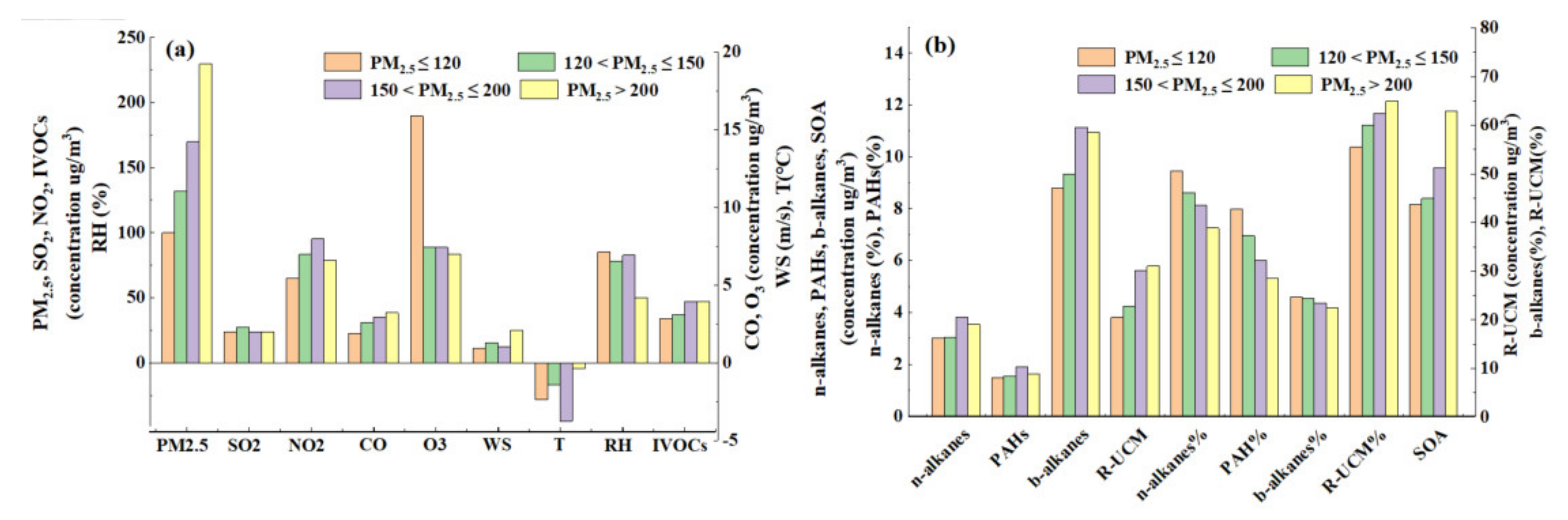
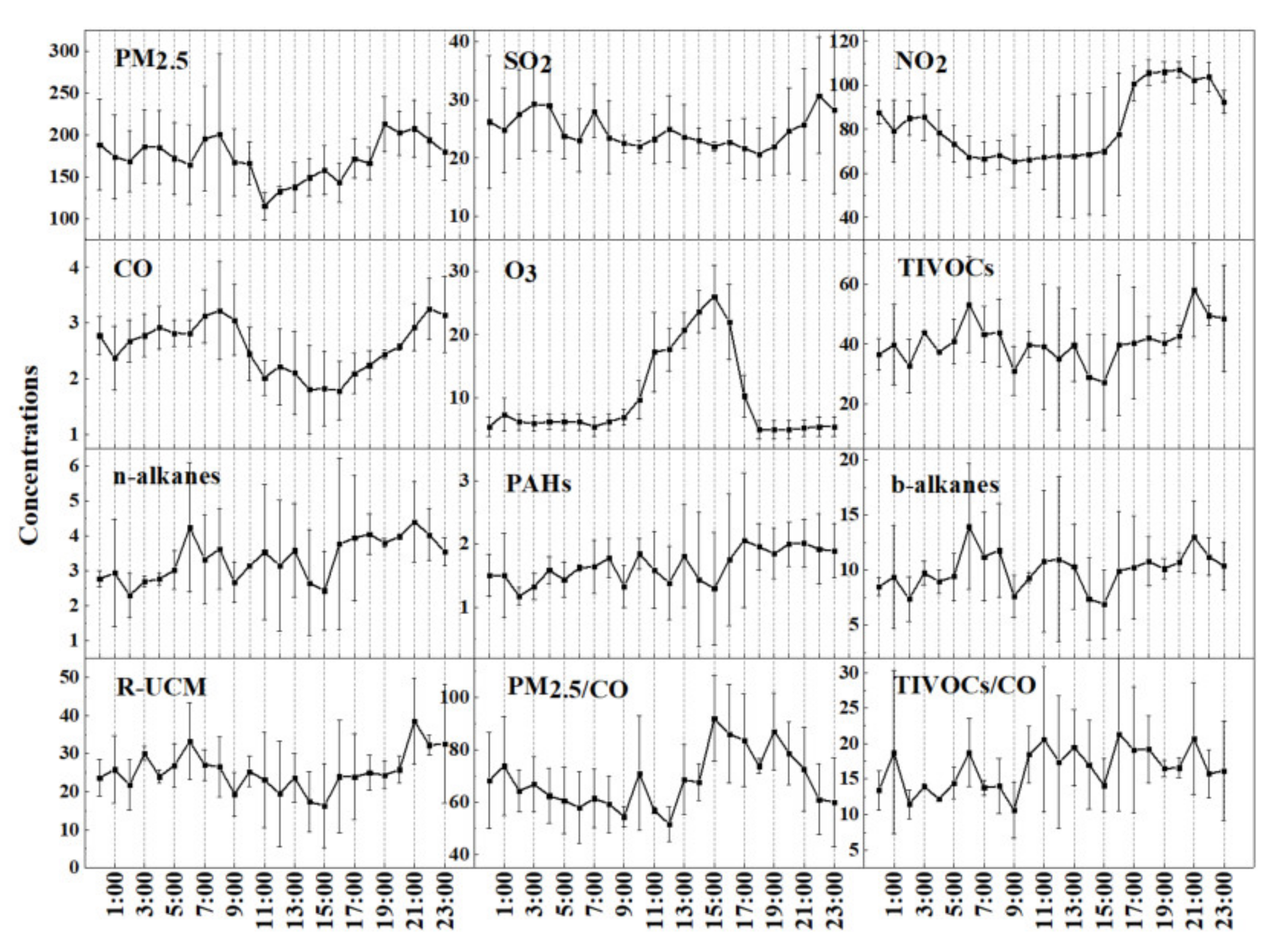
3.1. Concentration Levels of IVOCs during the Haze Episodes

Hourly time resolution samples of IVOCs and PM_2.5 were obtained during two haze episodes in Wangdu County, Hebei Province, defined as P1 (22–24 December 2019) and P2 (28–30 December 2019). The time series of the concentrations of IVOCs and PM_2.5 and the ratios of IVOCs’ components during haze episodes are shown in Figure 1. The temporal variation trend of IVOCs concentration was similar to that of PM_2.5 during haze episodes. However, these are not exactly consistent. The average concentration of IVOCs in P1 and P2 was 42.2 ± 14.8 μg·cm⁻³ (11.3~85.1 μg·cm⁻³) and 41.4 ± 12.2 μg·cm⁻³ (18.0~70.1 μg·cm⁻³), respectively, higher than that measured in Guangzhou (11.3 ± 7.8 μg·cm⁻³) [32], Yangshan Port in Shanghai during the G20 period (5.1 ± 0.8 μg·cm⁻³) [21], and Pasadena, California, in the summer (6.3 ± 1.9 μg·cm⁻³) [23], but lower than the values reported in Shanghai (58.5 ± 27.0 μg·cm⁻³) [22]. The concentration and fractional contributions of IVOCs components in P1 and P2 were similar. The average concentrations of n-alkanes (nC₁₂–nC₂₂) were 3.3 ± 1.3 μg·cm⁻³ and 3.6 ± 1.3 μg·cm⁻³, accounting for 8.2 ± 1.7% and 8.6 ± 1.6% of IVOCs, respectively. The average concentration of PAHs in P1 and P2 were 1.4 ± 0.5 μg·cm⁻³ and 2.1 ± 0.5 μg·cm⁻³, accounting for 3.6 ± 1.1% and 5.3 ± 1.0% of IVOCs, respectively. The average concentrations of b-alkanes (B₁₂~B₂₂ bins) in P1 and P2 were 10.4 ± 4.4 μg·cm⁻³ and 9.6 ± 3.2 μg·cm⁻³, accounting for 25.8 ± 4.5% and 23.2 ± 2.6% of IVOCs, respectively. R-UCM accounted for 85.6 ± 2.4% and 87.0 ± 2.8% of the IVOCs’ concentration in P1 and P2, respectively, which were similar to the case in Guangzhou [32]. Overall, the concentrations (fractional contributions to IVOCs mass) of n-alkanes, PAHs, b-alkanes, and R-UCM were 3.4 ± 1.3 μg·cm⁻³ (8.6 ± 2.3%), 1.7 ± 0.6 μg·cm⁻³ (6.8 ± 2.2%), 10.1 ± 3.9 μg·cm⁻³ (24.1 ± 3.8%), and 25.7 ± 9.9 μg·cm⁻³ (60.5 ± 6.5%) during haze episodes, respectively.

To further analyze the component characteristics of IVOCs with PM_2.5 pollution levels, four pollution stages (PM_2.5 ≤ 120 (I), 120 < PM_2.5 ≤ 150 (II), 150 < PM_2.5 ≤ 200 (III), PM_2.5 > 200 (IV)) were defined according to the PM_2.5 concentration and the number of samples (to divide as evenly as possible). The variations of gas-phase precursors and IVOCs components under different pollution conditions were analyzed and shown in Figure 2. From stages I to IV, the PM_2.5 concentration gradually increased from 100.0 ± 15.9 μg·cm⁻³ to 229.6 ± 29.9 μg·cm⁻³ and the IVOCs concentration increased gradually from 33.9 ± 19.1 μg·cm⁻³ to 47.3 ± 11.8 μg·cm⁻³. Therein, the concentration of n-alkanes, PAHs, and b-alkanes increased slowly from stage I to stage IV. However, the percentage of n-alkanes (from 9.5 ± 2.6% to 7.3 ± 1.1%), PAHs (from 8.0 ± 2.8% to 5.3 ± 1.1%), and b-alkanes (from 24.7 ± 4.6% to 22.5 ± 3.0%) in IVOCs gradually decreased from stage I to stage IV. By contrast, the absolute concentrations and relative contributions of the R-UCM increased significantly from stage I (20.5 ± 11.8 μg·cm⁻³, 55.5 ± 9.6%) to stage IV (31.1 ± 7.0 μg·cm⁻³, 64.9 ± 3.9%). These phenomena indicated that the aggravation of the haze episodes might be closely related to the unidentified IVOCs (i.e., R-UCM). Notably, the concentration of CO increased with the pollution degree, indicating that the haze episodes might be closely related to incomplete combustion sources. The O₃ concentration gradually decreased from stage I (15.9 ± 8.6 μg·cm⁻³) to stage IV (7.0 ± 2.9 μg·cm⁻³). It is speculated that IVOCs emission increased, leading to greater consumption of oxidants’ O₃. Meanwhile, SOA_IVOCs production of IVOCs was increased from 8.2 ± 2.7 μg·cm⁻³ to 11.8 ± 4.2 μg·cm⁻³. There was no direct linear relationship between PM_2.5 concentration and meteorological conditions such as SO₂, NO₂, WS, T, and RH, indicating differences in the causes of haze at different stages. For example, when PM_2.5 ≤ 120 μg·cm⁻³, low WS (0.9 ± 0.7 m/s) and high RH (85.1 ± 15.5%) conditions may be more conducive to the formation of the haze episode. When PM_2.5 > 200 μg·cm⁻³, the conditions of high WS (2.1 ± 1.1 m/s) and low RH (50.2 ± 17.9%) may be more conducive to the regional transport of pollutants and aggravate the haze episodes.

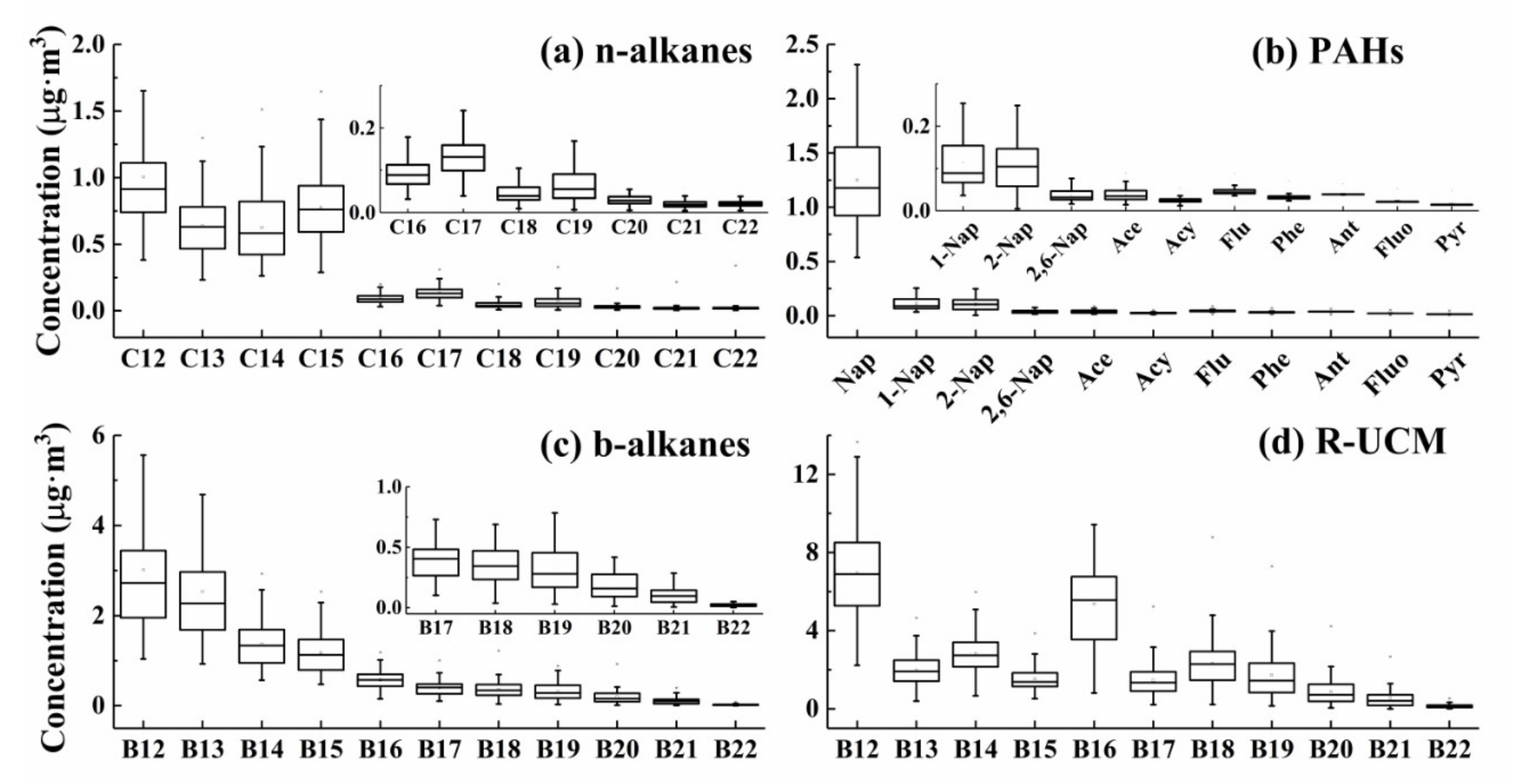
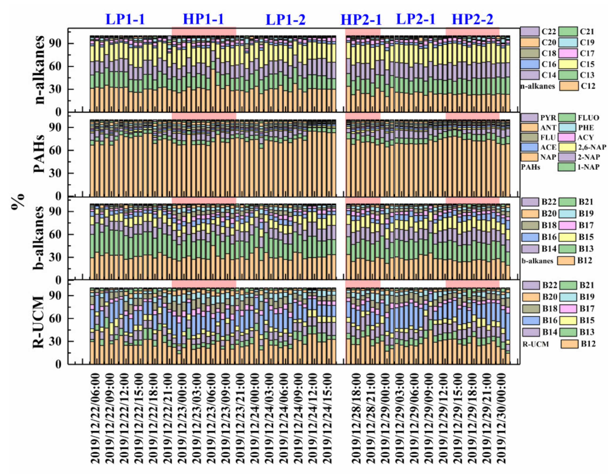
3.2. Component Characteristics of IVOCs during Haze Episodes

Figure 3 and Figure 4 showed the chemical profiles of the measured IVOCs during two haze episodes. Among n-alkanes, nC₁₂–nC₁₅ were the dominant species in n-alkanes, accounting for 87.4 ± 23.5% (nC₁₂: 28.6 ± 5.0%; nC₁₃: 18.3 ± 2.3%; nC₁₄: 18.0 ± 2.3%, and nC₁₅: 22.5 ± 2.9%, respectively). The proportion of nC₁₆~nC₂₂ showed a significant downward trend with the increase in the carbon number. Among PAHs, naphthalene and its alkyl substitutes were the primary species, accounting for 87.6 ± 2.9% of the measured PAHs. The proportions of 1-Nap, 2-Nap, and 2,6-Nap in PAHs were 4.1 ± 1.3%, 3.9 ± 2.1%, and 1.4 ± 1.4%, respectively. Overall, the distributions of n-alkanes and PAHs were basically consistent with previous studies [22]. The proportion of b-alkanes in B₁₂–B₁₆ bins was around 85.9 ± 5.4%. Meanwhile, R-UCMs in B₁₂–B₁₆ bins were the major components and constituted 74.0 ± 8.3% of the R-UCM in B₁₂–B₂₂ bins. The proportion of R-UCM showed a significant downward trend with the increase in the bins number. In addition, the percentages of Bn (B₁₂~B₂₂) in IVOCs during two haze episodes were 30.2 ± 5.4%, 13.3 ± 2.8%, 12.4 ± 2.3%, 8.9 ± 1.8%, 14.4 ± 4.5%, 4.8 ± 1.3%, 6.6 ± 2.3%, 4.9 ± 2.4%, 2.5 ± 1.3%, 1.7 ± 1.2%, and 0.4 ± 0.2% (Figure S3). Except for the B₁₆ bin, the proportion of each bin gradually decreases as the interval number increases. B₁₂~B₁₆ were the dominant bins among them, the sum of which account for 75.4 ± 18.2% of IVOCs. Xie et al. [33] reported that light n-alkanes with molecular weight < 282 and PAHs with a molecular weight < 192 almost exist in the form of gas in the ambient atmosphere. Therefore, the low molecular weight of n-alkanes, PAHs, b-alkanes, and R-UCM in the gas phase, that is, in IVOCs, showed higher mass concentrations than those of high molecular weight.

Temporal variations of different individual species in each type of IVOCs are shown in Figure 4. We defined the cases with PM_2.5 > 150 μg·cm⁻³ as the period of heavy pollution (HP, shown in the red background area in Figure 4), and others were defined as light pollution (LP) stages. The total concentration of IVOCs in HP (49.3 ± 12.4 μg·cm⁻³) was higher than that in LP (38.8 ± 10.3 μg·cm⁻³). The relative contributions of each IVOC component varied in HP and LP during two haze episodes are listed in Table S5. During the P1 haze, the proportion of n-alkanes, PAHs, and b-alkanes in LP was higher than that in HP, contrary to the component characteristics of P2 haze.

3.3. Sources of IVOCs

To further investigate the sources of IVOCs species during the haze episodes in this study, the component characteristics of IVOCs measured in the ambient atmosphere were firstly compared with the composition characteristics of IVOCs from source emissions reported by previous studies, including BB, CC, HFOV, NRCM, and GV/DV. Additionally, the composition characteristics of IVOCs in GV/DV unpublished from our research groups were included. Figure S4 showed the composition characteristics of IVOCs in various source emissions. Furthermore, the ratios of n-alkanes/b-alkanes in the ambient atmosphere were relatively stable and can better retain the ratio characteristics of emission sources, which was as the diagnosis ratio to identify the emission source. Moreover, the diurnal variation of IVOC components can also supply information on the emission source (Figure 5). Therefore, the source identification of IVOCs was from the three aspects mentioned above in this study.

In view of the fact that, like nC₁₆–nC₂₂ in n-alkanes; Flu, Phe, Ant, and Fluo in PAHs; b-alkanes in B₁₇–B₂₂ bins; and R-UCM in B₁₇–B₂₂ bins without obvious distinction in emission sources, the source identification of IVOCs was mainly based on the main compositions of IVOCs. The percentages of n-alkanes from nC₁₂ to nC₁₅ in n-alkanes accounted for 20.5–56.2%, 10.3–22.8%, 13.4–22.7%, and 10.7–29.4%, respectively, which were similar to the percentages in GV, DV, CC, and BB sources. Among PAHs, the proportion of Nap in PAHs was 67.7~85.2% higher than those from BB, CC, GV, DV, NRCM, and HFOV emissions. The possible explanation was that Nap might also come from other emissions, such as coking sources, resulting in high Nap concentration in an ambient atmosphere. The proportions of 1-Nap, 2-Nap, 2,6-NaP, and Acy were 4.5~9.7%, 0.5~11.3%, 1.6~2.9%, and 1.5~3.0%, respectively, which were similar to the emission characteristics of GV, BB and DV, GV, and GV, respectively. The percentages of b-alkanes in B₁₂–B₁₆ bins were 29.7 ± 4.2% (19.5~45.5%), 24.6 ± 4.1% (16.9~38.3%), 13.9 ± 2.1% (9.7~18.6%), 11.9 ± 2.3% (17.8~5.8%), and 5.8 ± 1.6% (3.0~11.8%), respectively. Those were similar to the distribution characteristics of BB, CC, DV, and GV sources. In general, the component characteristics of n-alkanes, PAHs, and b-alkanes in the ambient atmosphere were similar to GV, DV, BB, and CC; however, they were significantly different from the component characteristics of NRCM and HFOV sources. This might be because the sampling site was far from the ocean, and thus the contribution of HFOV and NRCM can be excluded.

The diurnal variation of IVOCs, especially n-alkanes, b-alkanes, and R-UCM, was generally consistent with those of PM_2.5, showing a lower concentration during the day (7:00~19:00) than that at night (20:00~6:00), which might be attributed to the influence of boundary layer height. IVOCs, n-alkanes, b-alkanes, and R-UCM had two peaks at 6:00 to 8:00 in the morning and 18:00 to 21:00 in the afternoon, corresponding to the morning and evening rush hours of vehicles. This was also consistent with the diurnal variation of the concentration of VOCs and NO₂ in the regional atmosphere, which showed “bimodal” distributions [34,35,36], indicating that vehicular emissions were a non-negligible emission source. Furthermore, since the sampling site is close to the national highway, vehicle emissions during the morning and evening exhibited more significant contributions to IVOCs. However, it is difficult to distinguish the contribution of GV and DV to IVOCs. The concentration of SO₂ at nighttime (26.6 ± 2.4 μg·cm⁻³) was generally higher than that during the daytime (23.1 ± 1.8 μg·cm⁻³), which might be attributed to the increased heating activities under low temperatures at night, leading to increased emissions from CC. Similarly, the concentration of CO at night was higher than that during the day. However, the diurnal variation of PAHs was relatively stable without peaks and valleys, which might be due to the synergic effects of vehicle sources during the day and combustion sources at night. In addition, IVOCs, n-alkanes, b-alkanes, and R-UCM appeared to have a low value between 13:00 and 16:00 due to the increased daytime illumination, O₃ concentration, and the intensity of the photochemical reaction; IVOCs were oxidized into SVOCs or SOA [23]. Moreover, the IVOC/CO ratio also peaked at 11:00–15:00, indicating that the contribution of secondary components of IVOCs increased during this period. The PM_2.5/CO ratio also peaked from 13:00 to 16:00, indicating that the proportion of secondary components in PM_2.5 increased significantly during this period due to the strong light and atmospheric photochemistry.

Table 1. Ratio of n-alkanes/b-alkanes in source emissions.

Emission Sources		n-Alkanes/b-Alkanes	Sampling Methods	References
Biomass burning	Rice straw	0.18	Laboratory simulation	Lu et al. [37]
	Pine wood	0.08	Laboratory simulation	Lu et al. [37]
	Crop straw	0.43 ± 0.17	Filed measurement	Qian et al. [13]
	Fuelwood	0.38 ± 0.12	Filed measurement
Coal combustion	Coal	0.57 ± 0.17	Filed measurement	Qian et al. [13]
	Coal	0.47 ± 0.09	Laboratory simulation	Lu et al. [37]
Gasoline emission	GV	0.10	On/off-road measurement	Zhao et al. [15]
	GV	0.83 ± 0.11	On-road measurement	Unpublished
	EGV	0.84 ± 0.35	On-road measurement
Diesel emission	DV	0.55 ± 0.26	On-road measurement	Unpublished
	DV	0.38	On-road measurement	Zhao et al. [16]
	HFOV	0.42	Filed measurement	Huang et al. [38]

listed the n-alkanes/b-alkanes ratios from various emission sources, including BB, CC, GV, DV, and HFOV. Notably, there was a significant difference in the ratios of n-alkanes/b-alkanes under the conditions of laboratory simulations and field measurements, which might cause uncertainties in source identification based on the ratios. Considering that the measured emission characteristics of combustion sources in the field were much closer to real combustion, the n-alkanes/b-alkanes ratio from field measurements was used for comparison. The ratios of n-alkanes/b-alkanes in P1 and P2 were 0.32 ± 0.03 and 0.37 ± 0.04, respectively, which were significantly higher than the ratios of BB in the laboratory simulated by Zhao et al. [16] and GV emission by Lu et al. [34]; however, they were lower than the field-measured values of GV and ethanol-gasoline vehicles (EGV) and close to the field-measured values of BB, CC, and DV. In short, this indicated that IVOCs during haze episodes might be influenced by complex contribution sources, such as the mixture of BB, CC, GV, and DV.

However, there are still great uncertainties in the source apportionment of IVOCs in an ambient atmosphere. On the one hand, the composition characteristics of IVOCs emission sources need to be further investigated. Meanwhile, the current IVOCs emission characteristics are only focused on four types of IVOCs species, including n-alkanes, PAHs, b-alkanes, and R-UCM, which cannot be used to effectively distinguish emission sources due to the lack of source-specific tracers. On the other hand, the sampling method of IVOCs needs to be improved. IVOCs sampling was based on Tenax TA adsorption tubes, which cannot effectively collect oxygen-containing IVOC (i.e., OIVOC) such as aldehydes, ketones, and acids. Such species are especially from BB and CC source emissions. According to previous studies, OIVOC may act as an important tracer for emission sources in the future. For example, Qian et al. [14] pointed out that methoxyphenols are unique in BB source emissions. However, no such substances were detected in ambient IVOC samples with a short sampling time in this study, which might be related to their low concentrations.

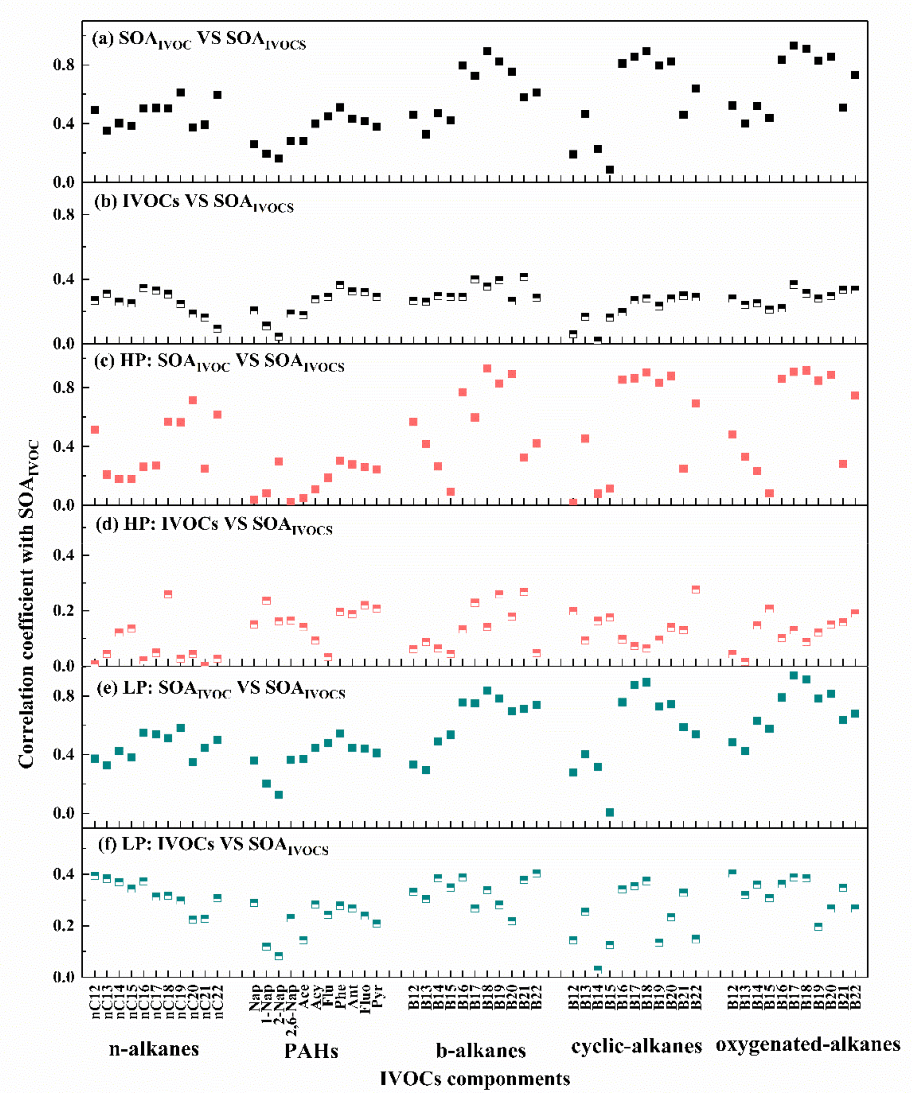
3.4. Estimation of SOA Production

IVOCs are important precursors of SOA, and SOA production estimated with different methods (e.g., SOA_IVOCs, SOA_OC/EC, and SOA_PMF) as mentioned in Section 2.3 is presented in Figure 6. It is clear that the variation in the trend of SOA_IVOCs estimated based on IVOCs was similar to that of IVOCs. SOA_IVOCs production in HP (10.3 ± 3.1 μg·cm⁻³) was higher than that of LP (8.2 ± 2.5 μg·cm⁻³), while SOA_OC/EC and SOA_PMF had similar trends during haze episodes. To be noted, SOA_IVOCs (9.2 ± 3.1 μg·cm⁻³) evaluated by IVOCs concentration were generally lower than SOA_OC/EC (23.3 ± 11.4 μg·cm⁻³) and SOA_PMF (22.7 ± 18.7 μg·cm⁻³). This could be attributed to the fact that IVOCs were included in the estimation of SOA_IVOCs, and there are other important SOA precursors such as VOCs that have not been considered. Moreover, it seems that SOA_OC/EC and SOA_PMF deviate more from SOA_IVOC and IVOCs in periods of HP than in those of LP. The reasons are as follows: the growth of SOA_OC/EC and SOA_PMF in the HP stage was smaller than in the LP stage. This was due to the increase in secondary inorganic components in the HP stage being the major factor for an increased pollution level rather than the increase in SOA components. However, the concentration of IVOCs and SOAIVOCs increases with the increase in pollution levels. Overall, the temporal variation trends of SOA_IVOCs, SOA_OC/EC, SOA_PMF, and IVOCs were consistent with hourly resolution data, as shown in Figure 6a.

To further analyze the relationships of different SOA productions, we transformed hourly resolution IVOCs into three hours for discussion, as shown in Figure 6b. Compared with the hourly resolution trend, a more consistent trend of SOA_IVOCs, SOA_OC/EC, and SOA_PMF was obtained in 3 h resolution; peaks appeared at 10:00–13:00 on 22 December, 20:00–22:00 on 22 December, 6:00–8:00 on 23 December, 21:00–23:00 on 23 December, 2:00–7:00 on 24 December, 10:00–16:00, and 19:00–22:00 on 29 December 2019. This phenomenon showed that the hourly resolution trend of different SOA production was more difficult to be fully captured compared with the 3 h resolution trend of SOA production, which implied the complex conversion mechanisms of IVOCs to SOA. In addition, as mentioned above, the values of SOA_IVOCs, SOA_OC/EC, and SOA_PMF were still different. It is difficult to establish direct relationships of IVOCs with different SOA productions, which is attributed to the synergic effect of various factors for the conversion of IVOCs to SOA, such as the different yields of IVOC components, meteorological conditions, atmospheric oxidation, hysteresis effect, etc.

To further explore the potential of IVOCs’ component contribution to SOA, the correlations of SOA_IVOC and IVOC components with SOA_IVOCs in the haze episodes (a, b), HP stages of haze (c, d), and LP stages of haze (e, f) are shown in Figure 7. During haze episodes, there is no significant difference in the correlation of n-alkanes, PAHs, b-alkanes, cyclic-alkanes, and oxygenated UCM with SOA_IVOCs; however, an obvious difference exists in its corresponding contribution of SOA_IVOC to SOA_IVOCs. Among them, the contribution of n-alkanes, PAHs, b-alkanes, cyclic-alkanes, and oxygenated alkanes to SOA_IVOCs were 0.86 ± 0.09 μg·cm⁻³ (9.5%), 0.41 ± 0.08 μg·cm⁻³ (4.6%), 1.27 ± 0.09 μg·cm⁻³ (14.1%), 4.44 ± 0.5 μg·cm⁻³ (49.3%), and 2.15 ± 0.20 μg·cm⁻³ (23.9%), respectively. Especially, the correlation of IVOCs corresponding SOA_IVOC with SOA_IVOCs showed a significant difference, such as the correlation coefficients of b-alkanes in B₁₆–B₂₀ bins, cyclic-alkanes in B₁₆–B₂₀ bins, and oxygenated UCM in B₁₆–B₂₀ bins with SOA_IVOCs being more than 0.6. Although the absolute concentrations of b-alkanes in B₁₂–B₁₅ bins were much higher than that of b-alkanes in B₁₆–B₂₀ bins (Figure 3), their contribution to SOA_IVOCs was relatively small. In HP, the correlation coefficients of IVOCs components with SOA_IVOCs were similar. Compared with the haze episodes, n-alkanes, PAHs, b-alkanes, cyclic-alkanes, and oxygenated alkanes in HP contributed 1.03 ± 0.10 μg·cm⁻³ (9.8%), 0.48 ± 0.09 μg·cm⁻³ (4.7%), 1.53 ± 0.09 μg·cm⁻³ (14.7%), 5.10 ± 0.48 μg·cm⁻³ (48.9%), and 2.57 ± 0.23 μg·cm⁻³ (24.7%) of SOA_IVOCs, which showed a higher concentration and similar contribution percentage of SOA_IVOCs. In particular, the correlation coefficients of the corresponding SOA_IVOC of nC₁₈–nC₂₀ in n-alkanes, b-alkanes in B₁₆–B₂₀ bins, cyclic-alkanes in B₁₆–B₂₀ bins, and oxygenated UCM in B₁₆–B₂₀ bins with SOA_IVOCs had increased, which meant that the increase in SOA_IVOCs in the HP stage was related to the outstanding contribution of the above components. The correlation of IVOCs components and their corresponding SOA_IVOC with SOA_IVOCs in the LP stage was similar to that of the haze episodes, which was due to the large time span of the LP stage in the haze episodes, which can strongly reflect the haze characteristics. N-alkanes, PAHs, b-alkanes, cyclic-alkanes, and oxygenated UCM in LP contributed 0.76 ± 0.08 μg·cm⁻³ (9.3%), 0.37 ± 0.07 μg·cm⁻³ (4.5%), 0.08 μg·cm⁻³ (13.6%), 4.04 ± 0.37 μg·cm⁻³ (49.4%), and 1.90 ± 0.17 μg·cm⁻³ (23.2%) of SOA_IVOCs, respectively. In short, compared with other components, b-alkanes, cyclic-alkanes, and oxygenated UCM in B₁₆–B₂₀ bins have greater potential to contribute to SOA_IVOCs in the hazing process, especially in the HP stage. However, the contribution of IVOCs to SOA_IVOCs was based on the same production rate for the same components under different pollution levels, which cannot be reflected in the actual contribution of each component of IVOCs to SOA_IVOCs production. In the future, the estimation of SOA_IVOCs production needs to comprehensively consider various factors such as meteorological conditions, atmospheric oxidation, and other factors, which reflect SOA production in a complex atmospheric environment.

4. Conclusions

In this study, two haze episodes with average PM_2.5 mass concentration up to 174.0 ± 49.0 μg·cm⁻³ were captured in Wangdu County, Hebei Province, North China, and the chemical characteristics and sources of IVOCs, as well as their associated contribution to SOA, were investigated during two haze episodes. The concentration of IVOCs measured in the ambient atmosphere was within the range of 11.3~85.1 μg·cm⁻³ during haze episodes. R-UCM (60.5 ± 6.5%) was a major part of IVOCs. The IVOCs concentration increased gradually with the increase in pollution levels, which might be closely related to the increase in the R-UCM concentration. Moreover, CC, BB, GV, and DV were identified as the important emission sources of IVOCs in Hebei Province based on the chemical characteristics of various emission sources and the hourly variation of IVOCs. Meanwhile, the overall temporal variations of SOA production estimated based on different methods were similar during haze episodes; however, their absolute concentrations differed.

In the future, the IVOCs sampling method needs to be improved to obtain unique tracers for each emission source and improve the accuracy of source apportionment of IVOCs. Especially, the identification and quantification of UCM components, including more oxygen, nitrogen, and sulfur compounds, such as phenols, furans, sugars, and acids, is an important and challenging work for the source identification of IVOCs, which can act as more efficient and unique source tracers to distinguish various emission sources. Moreover, there is still much to be explored in the future regarding the complex conversion mechanisms of IVOCs into SOA_IVOCs due to the influence of various factors such as the yield of different IVOC components, meteorological conditions, atmospheric oxidation, the hysteresis effect, etc.

References

1. Zhao, X.J.; Zhao, P.S.; Xu, J.; Meng, W.; Pu, W.W.; Dong, F.; He, D.; Shi, Q.F. Analysis of a winter regional haze event and its formation mechanism in the North China Plain. Atmos. Chem. Phys. Discuss. 2013, 13, 5685–5696. [Google Scholar] [CrossRef] [Green Version]
2. Liu, J.; Li, J.; Liu, D.; Ding, P.; Shen, C.; Mo, Y.; Wang, X.; Luo, C.; Cheng, Z.; Szidat, S.; et al. Source apportionment and dynamic changes of carbonaceous aerosols during the haze bloom-decay process in China based on radiocarbon and organic molecular tracers. Atmos. Chem. Phys. Discuss. 2016, 16, 2985–2996. [Google Scholar] [CrossRef] [Green Version]
3. Kautzman, K.E.; Surratt, J.D.; Chan, M.N.; Chan, A.W.H.; Hersey, S.P.; Chhabra, P.S.; Dalleska, N.F.; Wennberg, P.O.; Flagan, R.C.; Seinfeld, J.H. Chemical composition of gas- and aerosol-phase products from the photooxidation of naphthalene. J. Phys. Chem. A 2010, 114, 913–934. [Google Scholar] [CrossRef] [Green Version]
4. Yuan, B.; Hu, W.W.; Shao, M.; Wang, M.; Chen, W.T.; Lu, S.H.; Zeng, L.M.; Hu, M. VOC emissions, evolutions and contributions to SOA formation at a receptor site in eastern China. Atmos. Chem. Phys. Discuss. 2013, 13, 8815–8832. [Google Scholar] [CrossRef] [Green Version]
5. Couvidat, F.; Kim, Y.; Sartelet, K.; Seigneur, C.; Marchand, N.; Sciare, J. Modeling secondary organic aerosol in an urban area: Application to Paris, France. Atmos. Chem. Phys. Discuss. 2013, 13, 983–996. [Google Scholar] [CrossRef] [Green Version]
6. Presto, A.A.; Miracolo, M.A.; Kroll, J.H.; Worsnop, D.R.; Robinson, A.L.; Donahue, N.M. Intermediate-Volatility Organic Compounds A Potential Source of Ambient Oxidized Organic Aerosol. Environ. Sci. Technol. 2019, 43, 4744–4749. [Google Scholar] [CrossRef]
7. Huang, G.; Liu, Y.; Shao, M.; Li, Y.; Chen, Q.; Zheng, Y.; Wu, Z.; Liu, Y.; Wu, Y.; Hu, M.; et al. Potentially Important Contribution of Gas-Phase Oxidation of Naphthalene and Methylnaphthalene to Secondary Organic Aerosol during Haze Events in Beijing. Environ. Sci. Technol. 2019, 53, 1235–1244. [Google Scholar] [CrossRef] [PubMed]
8. Chan, A.W.H.; Kautzman, K.E.; Chhabra, P.S.; Surratt, J.D.; Chan, M.N.; Crounse, J.D.; Kürten, A.; Wennberg, P.O.; Flagan, R.C.; Seinfeld, J.H. Secondary organic aerosol formation from photooxidation of naphthalene and alkylnaphthalenes: Implications for oxidation of intermediate volatility organic compounds (IVOCs). Atmos. Chem. Phys. 2009, 9, 3049–3060. [Google Scholar] [CrossRef] [Green Version]
9. Pye, H.O.T.; Seinfeld, J.H. A global perspective on aerosol from low-volatility organic compounds. Atmos. Chem. Phys. Discuss. 2010, 10, 4377–4401. [Google Scholar] [CrossRef] [Green Version]
10. Zhao, B.; Wang, S.; Donahue, N.M.; Jathar, S.H.; Huang, X.; Wu, W.; Hao, J.; Robinson, A. Quantifying the effect of organic aerosol aging and intermediate-volatility emissions on regional-scale aerosol pollution in China. Sci. Rep. 2016, 6, 28815. [Google Scholar] [CrossRef] [PubMed] [Green Version]
11. Pye, H.O.T.; Pouliot, G. Modeling the Role of Alkanes, Polycyclic Aromatic Hydrocarbons, and Their Oligomers in Secondary Organic Aerosol Formation. Environ. Sci. Technol. 2012, 46, 6041–6047. [Google Scholar] [CrossRef]
12. Woody, M.C.; West, J.J.; Jathar, S.H.; Robinson, A.L.; Arunachalam, S. Estimates of non-traditional secondary organic aerosols from aircraft SVOC and IVOC emissions using CMAQ. Atmos. Chem. Phys. Discuss. 2015, 15, 6929–6942. [Google Scholar] [CrossRef] [Green Version]
13. Qian, Z.; Chen, Y.; Liu, Z.; Han, Y.; Zhang, Y.; Feng, Y.; Shang, Y.; Guo, H.; Li, Q.; Shen, G.; et al. Intermediate Volatile Organic Compound Emissions from Residential Solid Fuel Combustion Based on Field Measurements in Rural China. Environ. Sci. Technol. 2021, 55, 5689–5700. [Google Scholar] [CrossRef]
14. Cai, S.; Zhu, L.; Wang, S.; Wisthaler, A.; Li, Q.; Jiang, J.; Hao, J. Time-Resolved Intermediate-Volatility and Semivolatile Organic Compound Emissions from Household Coal Combustion in Northern China. Environ. Sci. Technol. 2019, 53, 9269–9278. [Google Scholar] [CrossRef]
15. Zhao, Y.; Nguyen, N.T.; Presto, A.A.; Hennigan, C.J.; May, A.; Robinson, A. Intermediate Volatility Organic Compound Emissions from On-Road Gasoline Vehicles and Small Off-Road Gasoline Engines. Environ. Sci. Technol. 2016, 50, 4554–4563. [Google Scholar] [CrossRef]
16. Zhao, Y.; Nguyen, N.T.; Presto, A.A.; Hennigan, C.J.; May, A.; Robinson, A. Intermediate Volatility Organic Compound Emissions from On-Road Diesel Vehicles: Chemical Composition, Emission Factors, and Estimated Secondary Organic Aerosol Production. Environ. Sci. Technol. 2015, 49, 11516–11526. [Google Scholar] [CrossRef] [PubMed]
17. Cross, E.S.; Sappok, A.G.; Wong, V.W.; Kroll, J.H. Load-Dependent Emission Factors and Chemical Characteristics of IVOCs from a Medium-Duty Diesel Engine. Environ. Sci. Technol. 2015, 49, 13483–13491. [Google Scholar] [CrossRef] [PubMed]
18. Lou, H.; Hao, Y.; Zhang, W.; Su, P.; Zhang, F.; Chen, Y.; Feng, D.; Li, Y. Emission of intermediate volatility organic compounds from a ship main engine burning heavy fuel oil. J. Environ. Sci. 2019, 84, 197–204. [Google Scholar] [CrossRef]
19. Qi, L.; Liu, H.; Shen, X.; Fu, M.; Huang, F.; Man, H.; Deng, F.; Shaikh, A.A.; Wang, X.; Dong, R.; et al. Intermediate-Volatility Organic Compound Emissions from Nonroad Construction Machinery under Different Operation Modes. Environ. Sci. Technol. 2019, 53, 13832–13840. [Google Scholar] [CrossRef] [PubMed]
20. Cross, E.S.; Hunter, J.F.; Carrasquillo, A.J.; Franklin, J.P.; Herndon, S.C.; Jayne, J.T.; Worsnop, D.R.; Miake-Lye, R.C.; Kroll, J.H. Online measurements of the emissions of intermediate-volatility and semi-volatile organic compounds from aircraft. Atmos. Chem. Phys. Discuss. 2013, 13, 7845–7858. [Google Scholar] [CrossRef] [Green Version]
21. Wang, P.P.; Li, Y.J.; Zhang, F.; Chen, Y.J.; Feng, Y.L.; Xu, J.M.; Ma, Y.G.; Huang, C.; Li, L.; Li, J.; et al. Concentration, composition and variation of ambient IVOCs in Shanghai Port during the G20 summit. GEOCHIMICA 2018, 47, 313321. [Google Scholar]
22. Li, Y.; Ren, B.; Qiao, Z.; Zhu, J.; Wang, H.; Zhou, M.; Qiao, L.; Lou, S.; Jing, S.; Huang, C.; et al. Characteristics of atmospheric intermediate volatility organic compounds (IVOCs) in winter and summer under different air pollution levels. Atmos. Environ. 2019, 210, 58–65. [Google Scholar] [CrossRef]
23. Zhao, Y.; Hennigan, C.; May, A.; Tkacik, D.S.; de Gouw, J.; Gilman, J.B.; Kuster, W.; Borbon, A.; Robinson, A. Intermediate-Volatility Organic Compounds: A Large Source of Secondary Organic Aerosol. Environ. Sci. Technol. 2014, 48, 13743–13750. [Google Scholar] [CrossRef] [PubMed]
24. Cui, M.; Chen, Y.; Tian, C.; Zhang, F.; Yan, C.; Zheng, M. Chemical composition of PM 2.5 from two tunnels with different vehicular fleet characteristics. Sci. Total Environ. 2016, 550, 123–132. [Google Scholar] [CrossRef]
25. Cui, M.; Chen, Y.; Feng, Y.; Li, C.; Zheng, J.; Tian, C.; Yan, C.; Zheng, M. Measurement of PM and its chemical composition in real-world emissions from non-road and on-road diesel vehicles. Atmos. Chem. Phys. Discuss. 2017, 17, 6779–6795. [Google Scholar] [CrossRef] [Green Version]
26. Lv, L.; Chen, Y.; Han, Y.; Cui, M.; Wei, P.; Zheng, M.; Hu, J. High-time-resolution PM2.5 source apportionment based on multi-model with organic tracers in Beijing during haze episodes. Sci. Total Environ. 2021, 772, 144766. [Google Scholar] [CrossRef] [PubMed]
27. Hopke, P.K. Review of receptor modeling methods for source apportionment. J. Air Waste Manag. Assoc. 2015, 66, 237–259. [Google Scholar] [CrossRef] [PubMed]
28. Paatero, P. The multilinear engine—A table-driven, least squares program for solving multilinear problems, including the n-way parallel factor analysis model. J. Comput. Graph. Stat. 1999, 8, 854–888. [Google Scholar]
29. Aumont, B.; Valorso, R.; Mouchel-Vallon, C.; Camredon, M.; Lee-Taylor, J.; Madronich, S. Modeling SOA formation from the oxidation of intermediate volatility n-alkanes. Atmos. Chem. Phys. 2012, 12, 7577–7589. [Google Scholar] [CrossRef] [Green Version]
30. Cao, J.; Lee, S.; Ho, K.F.; Zou, S.; Fung, K.; Li, Y.; Watson, J.; Chow, J.C. Spatial and seasonal variations of atmospheric organic carbon and elemental carbon in Pearl River Delta Region, China. Atmos. Environ. 2004, 38, 4447–4456. [Google Scholar] [CrossRef]
31. Yu, S.; Dennis, R.L.; Bhave, P.V.; Eder, B.K. Primary and secondary organic aerosols over the United States: Estimates on the basis of observed organic carbon (OC) and elemental carbon (EC), and air quality modeled primary OC/EC ratios. Atmos. Environ. 2004, 38, 5257–5268. [Google Scholar] [CrossRef]
32. Tang, T.G. Characteristics and Source Apportionment of Atmospheric Intermediate-Volatility Organic Compounds (IVOCs) in Selected Chinese Cities. Ph.D. Thesis, Guangzhou Institute of Geochemistry, Chinese Academy of Sciences, Guangzhou, China, 2020. (In Chinese). [Google Scholar]
33. Xie, M.; Hannigan, M.; Barsanti, K. Gas/particle partitioning of n-alkanes, PAHs and oxygenated PAHs in urban Denver. Atmos. Environ. 2014, 95, 355–362. [Google Scholar] [CrossRef]
34. Mozaffar, A.; Zhang, Y.-L.; Fan, M.; Cao, F.; Lin, Y.-C. Characteristics of summertime ambient VOCs and their contributions to O3 and SOA formation in a suburban area of Nanjing, China. Atmos. Res. 2020, 240, 104923. [Google Scholar] [CrossRef]
35. Zhang, Y.; Li, R.; Fu, H.; Zhou, D.; Chen, J. Observation and analysis of atmospheric volatile organic compounds in a typical petrochemical area in Yangtze River Delta, China. J. Environ. Sci. 2018, 71, 233–248. [Google Scholar] [CrossRef]
36. Olumayede, E.G. Atmospheric Volatile Organic Compounds and Ozone Creation Potential in an Urban Center of Southern Nigeria. Int. J. Atmos. Sci. 2014, 2014, 1–7. [Google Scholar] [CrossRef]
37. Lu, Y.J.; Feng, Y.L.; Qian, Z.; Han, Y.; Chen, Y.J. Emission Characteristics of IVOCs from the Combustion of Residential Solid Fuels and the Impact of Burning Temperature. Environ. Sci. 2019, 40, 4404–4411. [Google Scholar]
38. Huang, C.; Hu, Q.; Li, Y.; Tian, J.; Ma, Y.; Zhao, Y.; Feng, J.; An, J.; Qiao, L.; Wang, H.; et al. Intermediate Volatility Organic Compound Emissions from a Large Cargo Vessel Operated under Real-World Conditions. Environ. Sci. Technol. 2018, 52, 12934–12942. [Google Scholar] [CrossRef] [PubMed]
Figure 1. Time series of the concentrations of IVOCs, PM2.5, and the fractional contributions of different types of IVOCs components during haze episodes.
Atmosphere 12 01484 g001
Figure 2. Characteristics of gaseous precursors, IVOCs components, and contribution to SOA at different pollution stages. (a) The concentration of PM2.5, IVOCs, SO2, NO2, CO, and O3 and meteorological parameters such as WS, RH, and T; (b) the concentration of n-alkanes, PAHs, b-alkanes, R-UCM, and SOA, and the corresponding ratios in IVOCs.
Atmosphere 12 01484 g002
Figure 3. Component concentrations of (a) n-alkanes, (b) PAHs, (c) b-alkanes, and (d) R-UCM. (The top to the bottom of the box chart represents the maximum, quartile, median, lower quartile, and minimum of the concentration of each species. B-alkanes and R-UCM are the parts of each bin with the same X-coordinate axis).
Atmosphere 12 01484 g003
Figure 4. Temporal variations of the fractional contributions of individual species in n-alkanes, PAHs, b-alkanes, and R-UCM in IVOCs (heavy pollution with PM2.5 > 150 μg·cm−3 was defined as HP; light pollution with PM2.5 > 150 μg·cm−3 was defined as LP; HP/LP in P1 and P2 were defined as HP1/LP1 and HP2/LP2, respectively).
Atmosphere 12 01484 g004
Figure 5. Diurnal variations of PM2.5, gaseous precursors, and IVOC components during the haze episodes.
Atmosphere 12 01484 g005
Figure 6. Time series of different SOA productions during haze episodes with (a) hourly resolution and (b) 3 h resolution.
Atmosphere 12 01484 g006
Figure 7. Correlation coefficient (r)of IVOCs components and its corresponding SOAIVOC with SOAIVOCs in haze episodes (black rectangle represents the haze episodes; pink rectangle represents HP stage; green rectangle represents LP stage; SOAIVOC represents the individual IVOC production, SOAIVOCs respesents the total IVOCs production) (a): SOAIVOC vs. SOAIVOCs and (b): IVOCs vs. SOAIVOCs, HP stages of haze. (c): SOAIVOC vs. SOAIVOCs and (d): IVOCs vs. SOAIVOCs and LP stages of haze. (e): SOAIVOC vs. SOAIVOCs and (f): IVOCs vs. SOAIVOCs.
Atmosphere 12 01484 g007