Article

Stress-Induced Apparent Resistivity Variations at the Kalpin Observatory and the Correlation with the 2020 Mw 6.0 Jiashi Earthquake

1
China Earthquake Networks Center, Beijing 100045, China
2
Earthquake Agency of The Xinjiang Uygur Autonomous Region, Urumqi 830011, China
3
Xinjiang Institute of Engineering, Urumqi 830023, China
*
Author to whom correspondence should be addressed.
Atmosphere 2021, 12(11), 1420; https://doi.org/10.3390/atmos12111420
Submission received: 16 September 2021 / Revised: 18 October 2021 / Accepted: 26 October 2021 / Published: 28 October 2021

Abstract

:
Stress may induce apparent resistivity changes. Clarifying the deformation process of the source media is critical for determining the correlations between resistivity variations and earthquake occurrence. In this study, the stress state of a medium was analyzed by integrating GPS measurements, the spatiotemporal evolution of the load/unload response ratio (LURR), geochemical monitoring, and synchronous apparent resistivity changes preceding the 2020 Mw 6.0 Jiashi earthquake. The medium hosting the Kalpin Observatory underwent elastic deformation before 2019, and the synchronous decreases in the E–W and N–S apparent resistivities from 2015 can be attributed to N–S-dominated compressive stress. The microdamage stage occurred in 2019, with subsequent E–W apparent resistivity variation amplitudes that were ~0.4 Ωm higher than those in previous years. This difference is a result of microdamage to the medium owing to tensile stress during the seismogenic process. The spatiotemporal evolution of the LURR and gas seepage monitoring data also indicate that the medium was damaged prior to the earthquake. Variations in the apparent resistivity measured at the Kalpin Observatory indicate that the medium underwent elastic deformation, followed by microdamage, until stress triggered the earthquake.

1. Introduction

Resistivity is an important physical property of geotechnical materials that varies with stress [1,2,3,4]. According to data from laboratory experiments, mechanical stress can narrow or widen cracks in rocks and alter the distribution of conductive solutions in cracks, thereby affecting the rock resistivity [5,6,7,8,9]. Earthquakes result from deformation and damage to a medium via continuous stress loading. The seismogenic process is accompanied by changes in the physical parameters of the underground media [10]. A 50% decrease in the resistivity occurred along deep portions of the San Andreas Fault from 1986 [11]. Four years prior to the 1976 Tangshan earthquake, a gradual decrease in the apparent resistivity of the shallow crust was observed at multiple sites [12,13]. A gradual apparent resistivity decrease of up to 6.7% several years prior to the 2008 Wenchuan earthquake was recorded at Pixian station [14]. Researchers have determined that some variations in the apparent resistivity were associated with earthquakes in the Garm region [15]. Temporal changes in resistivity before and after the Izmit (Mw 7.6) earthquake have also been reported [16]. Hautot [17] reported resistivity changes in the Sur-Frêtes ridge, which correlated with mechanical stress caused by changes in the lake level. Based on the fluid distribution underneath the hypocentral region, which is well known as a fluid valve model of Sibson [18], some researchers have claimed that temporal resistivity changes observed using magnetotellurics can reflect fluid movement in the hypocentral region [19,20,21].
In China, shallow apparent resistivity detection began in 1966. There are more than 80 continuous apparent resistivity stations currently in operation. Prior to some large earthquakes, significant resistivity changes have been observed and reported later [12,14,22,23,24]. Thus, studying changes in shallow apparent resistivity related to earthquakes is still of great significance for capturing seismic signals.
Although many studies have linked resistivity changes to stress [13,25,26], capturing the precursory changes that occur prior to an earthquake remains challenging. This is mainly because the relationship between resistivity changes and stress is complex, with varying resistivity characteristics present in different stress states. For example, although the resistivity of a water-bearing rock decreases significantly under high stress, both decreases and increases in resistivity have been reported at low stress levels [1,2,5,8,27,28,29,30,31]. The complexity of resistivity variations is likely associated with the difficulty of obtaining the source properties, mechanical state, and deformation state of the medium during the seismogenic process [32]. Therefore, determining the deformation state of a medium is an important step for establishing correlations between changes in apparent resistivity and earthquakes.
Based on the deformation states of rocks during stress loading, Ma et al. [33] partitioned the seismogenic process into the following stages: elastic deformation, yield, meta-instability, and instability (failure). According to Scholz [34], a medium experiences elastic strain buildup, dilatancy-dominated, and water influx-dominated stages. Considering the constitutive law for rocks [35], during the initial stress loading stage (when the rock is in the elastic stage), the loading and unloading response rates (deformation modulus) are approximately equal. However, when the stress accumulation increases, the rock enters the yield stage and its loading response rate exceeds that of unloading. This decreases the strength of the rock or damages it, eventually causing failure. This mechanism has been exploited to propose a method for quantitatively describing the stage of damage to a medium, known as the load/unload response ratio (LURR) [35,36,37]. Abnormal LURRs have been reported for months to years prior to large earthquakes [35,36,38]. Therefore, the evolution of the LURR reflects the deformation state and the evolution of damage within a medium.
On 19 January 2020, the Jiashi Mw 6.0 earthquake occurred in the Atushi–Kalpin Thrust Zone, southern Tien Shan Mountain at the depth of 14.9 km. This area (Figure 1) hosts the Kalpin Apparent Resistivity Observatory, a baseline geodetic survey observatory, a geochemical monitoring campaign, and several GPS monitoring sites. To determine the correlation between apparent resistivity changes and the Jiashi Mw 6.0 earthquake, the spatiotemporal evolution of the LURR, GPS strain monitoring, and synchronous gas seepage data were utilized in this study to investigate the deformation state of the medium in the seismogenic region. The variations in the apparent resistivity under different stress states were also analyzed.

2. Geologic Setting and Environment of Observatory

2.1. Tectonic Setting

The Tien Shan orogenic belt undergoes strong active deformation that is characterized by nearly N–S crustal shortening and uplift. Several reverse faults and fold belts are present in the northern and southern Tien Shan Mountains [39]. The latest crustal defor mation in this region has been attributed to remote strain caused by the collision of the Indian and Eurasian tectonic plates. The Atushi–Kalpin Thrust Zone is located in the western South Tien Shan Seismic Belt and the Kuche Depression, which includes the Kashi Depression and the Bachu Uplift [40]. The Kalpin thrust system is divided into two parts by the transform-like strike-slip Piqiang Fault. The western part of the system comprises the Kalpintag (KPT), Aozigertawu (AZT), Toksanatanengbayler (TST), Kekebuke Sanshan (KST), and Aoyibulake (AYT) thrust faults. The eastern part of the system includes the KPT, Tataiertage (TAT), Yimugantawu (YMT), TST, KST, and AYT thrust faults from south to north [39] (Figure 1). According to Yang et al. [41], the crust in the Kalpin Thrust Zone has shortened by 40–45 km since the Cenozoic Era, indicating a shortening rate of 33–37%.
The KPT is the foremost (southern) thrust fault in the Atushi–Kalpin Thrust Zone, comprising an overturned fold-and-front thrust that extends over a lateral distance of 220 km [42,43,44]. Based on an integrated analysis of the surface geology, topography, focal mechanisms, seismic reflection profiles, and InSAR co-seismic deformation, Yao et al. [45] determined that the 19 January 2020 Jiashi Mw 6.0 earthquake occurred on the KPT Thrust Fault.

2.2. Kalpin Apparent Resistivity Observatory

The Kalpin Apparent Resistivity Observatory is located in the Atushi–Kalpin Thrust Zone. A ZD8M resistivity monitoring system, with two quasi-Schlumberger arrays (transmitting dipole AB and receiving dipole MN) aligned N–S and E–W, is installed at the observatory. The distances between transmitting dipoles A and B in the N–S and E–W directions are 1004 m and 1007 m, respectively (Figure 2). This autonomous system records hourly resistivity data. The monitoring field is on the edge of the Gobi Desert, and an abandoned hydropower station, a sinking pond, an irrigation well, and a transformer is located around the station. Considering that these sites are located outside the range of the two quasi-Schlumberger arrays, their interference with the apparent resistivity observations is negligible. Owing to the high-porosity medium present in the observation field, the apparent resistivity is sensitive to stress.
The resistivities of rocks in the upper crust mainly depend on the mobility of ions and the distribution of fluids. Conductivity is generated in sediments via current flowing through fluid-filled pores or along the surfaces of clay minerals [25]. Therefore, precipitation and other nontectonic processes affect the resistivity of sediment. Considering the climatic characteristics of mainland China, elevated summer precipitation often decreases the resistivity. Therefore, resistivity data from most stations decreased during the rainy season (July–September), followed by an increase during the dry season (December–March). However, data from some stations (e.g., Pixian Station in Sichuan Province) exhibited an inverse annual pattern, in which the apparent resistivity increased during the rainy season and decreased during the dry season [46]. The apparent resistivity data from the Kalpin Observatory were also characterized by an abnormal annual pattern, i.e., the apparent resistivity was high when precipitation was high and low when the precipitation was low.

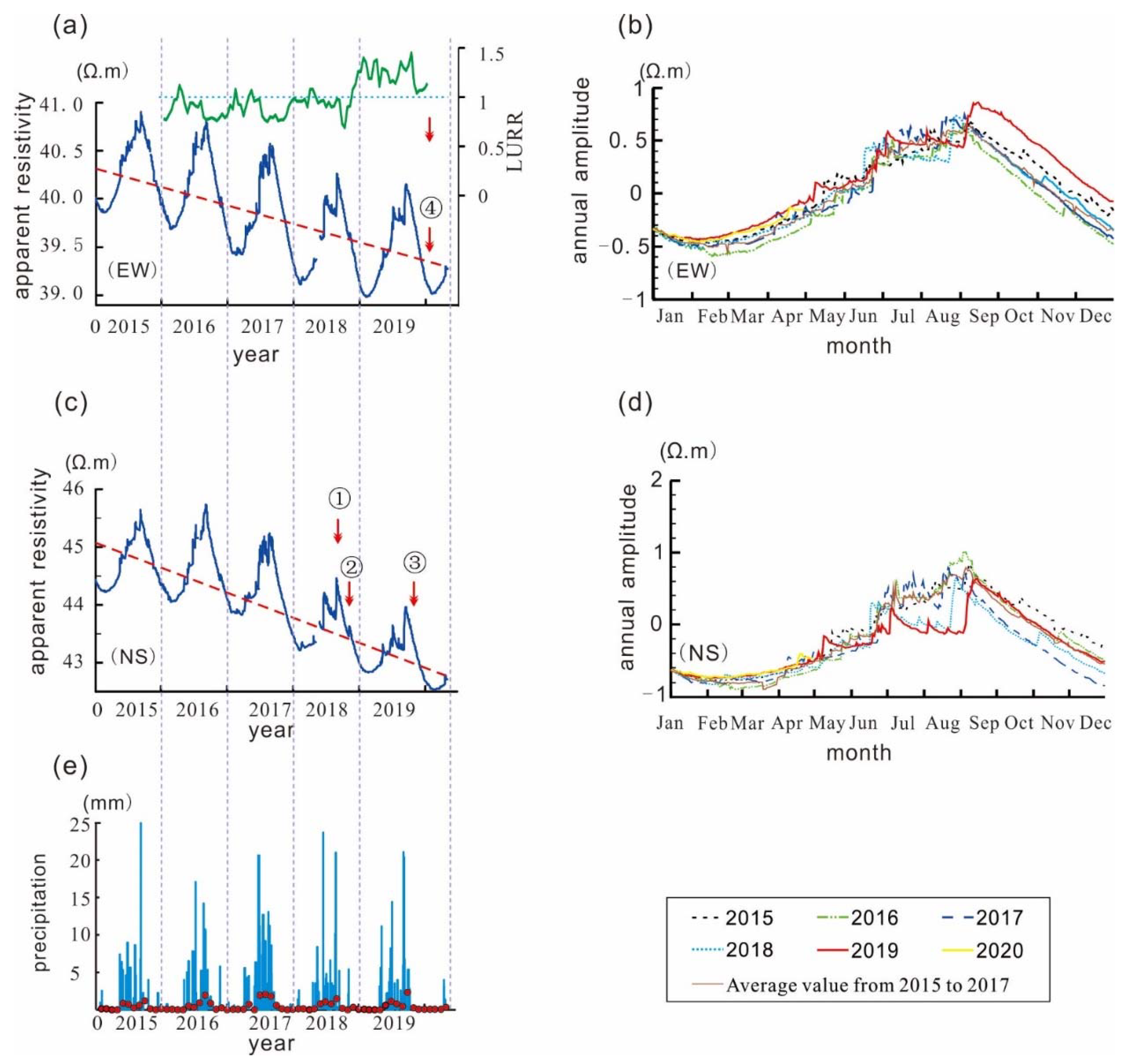
3. Variations Recorded at the Kalpin Observatory

Figure 3a,c display plots of the mean daily apparent resistivity values recorded at the Kalpin Observatory from January 2015 to April 2020. The apparent resistivity exhibited a monotonic decrease in both the N–S and E–W directions from 2015, with a decreasing rate of 0.17 Ωm/a in the E–W direction and 0.35 Ωm/a in the N–S direction. The apparent resistivity in the N–S direction decreased approximately twice as fast as that of the E–W direction. Figure 3b,d show the annual variations and amplitudes of the apparent resistivity, respectively, recorded in the E–W and N–S directions at the Kalpin Observatory, which were extracted using a polynomial fitting method. We fitted the data using the first-order polynomials to obtain the decreasing trend of apparent resistivity. Then the decreasing trend was subtracted from the data. We finally plotted remaining data with the same time scale of one year, as shown in Figure 3b,d.
From 15 June to 25 August 2018, the N–S variations were significantly lower than the average values in previous years, after which they returned to the average level observed in previous years. Subsequently, the Jiashi Ms 5.5 (4 September 2018) and the Atushi Ms 5.1 earthquakes (4 November 2018) occurred in the Atushi–Kalpin Thrust Zone. From 20 June 2019 to 15 September 2019, the apparent resistivity in the N–S direction was again lower than the previous average values, which lasted for 87 d (Figure 3d). Following the return to normal apparent resistivity values, the Wushi Ms 5.0 earthquake occurred on 27 October 2019. From September 2019 onward, the annual variations in apparent resistivity measured in the E–W direction surpassed those observed in previous years by ~0.4 Ωm. This lasted until 19 January 2020 (0138 d), which coincided with the occurrence of the Jiashi Mw 6.0 earthquake (Figure 3b).
As precipitation typically affects the apparent resistivity measurements, we assessed the precipitation data collected at the Kalpin Meteorological Observatory, which is located less than 5 km from the apparent resistivity observatory, between 1 January 2015 and 30 April 2020 to exclude the potential interference (Figure 3e). We found that there was a good correlation between precipitation and apparent resistivity, i.e., when the precipitation was high, the resistivity was also high, and when precipitation was low, the apparent resistivity was low. The data yielded an average annual precipitation of 160.32 mm from 2015 to 2019, with annual averages of 148.9 and 171.8 mm for 2018 and 2019, respectively, which are comparable to the amounts recorded in previous years.

4. Local Stress Environment

In order to describe the local crustal movement in more detail, we calculated the GPS strain rates based on the distance weighting method [39,40]. The study area was divided into uniform grids and the horizontal velocity gradient of each grid point was calculated one by one.
U i = t i + u i x j x j = t i + e i j x j
where, U i denotes the velocity of the GPS sites, t i denotes the fitted velocity of the grid point, x j denotes the distance between the grid point and the corresponding GPS sites, and e i j   is the velocity gradient tensor.
After adjustment of the calculation, the maximum and minimum principal strain rates were calculated by the following formula.
ε i j = e i j + e j i 2
ε 1 , 2 = e x x + e y y 2 ± ( e x x e y y 2 ) 2 + ( e x y ) 2
where ε i j is the strain rate tensor, and ε 1 , 2 are the maximum and minimum principal strain rates.
We calculated the strain rates for the Tien Shan orogenic belt using GPS data collected from 2015 to 2019. The results indicated that N–S compression occurred in the Tien Shan Mountains. The strain rates to the SW and NE of the Atushi–Kalpin Thrust Zone were high, with maximum principal strain rates that exceeded −5 × 10⁻⁸/y. In the central region, the maximum principal strain rate decreased to approximately −1 × 10⁻⁸/y (Figure 4a). The crust in the Tarim Basin, which is located southeast of Kalpin, was characterized by tension. The Kalpin Apparent Resistivity Observatory is located in a transition zone between the compressional and tensional regimes, which explains its relatively low strain rate of –1.89 × 10⁻⁸/yr. The maximum principal strain at Kalpin also exhibited a N–S trend, with strain rates of –1.80 × 10⁻⁸ and –0.57 × 10⁻⁸/yr for the N–S and E–W components, respectively (Figure 4b).
Wang and Shen [47] processed GPS data collected during the past 25 years (until 2016) for continental China and found that the dilatation rates indicate areal contraction of up to 40 nanostrains/y across the Tien Shan region. This orogenic belt has been characterized by continuous compression [47] and the GPS-derived data used herein also indicated that the Atushi–Kalpin Thrust Zone was under compressive deformation, similar to the period before 2016.
Geodetic baselines in the Atushi–Kalpin Thrust Zone (Figure 1) include the NNE trending Wuqia–Yecheng and Bachu–Wushi, and the E–W trending Bachu-Wuqia. Li et al. [48] analyzed data from these baselines, which indicated that N–S compression has remained the dominant stress component since 2017 in the Atushi–Kalpin Thrust Zone.
Three recent earthquakes of Ms ≥ 5.0, excluding the Jiashi Mw 6.0 earthquake, occurred in the Atushi–Kalpin Thrust Zone (Figure 1). Based on the focal mechanism solutions issued by the U.S. Geological Survey and Harvard University (see Data and Resources), the principal stress direction of the Jiashi Ms 5.0 earthquake on 4 September 2018, was roughly N–S, whereas those of the Atushi Ms 5.1 on 4 November 2018, and the Wushi Ms 5.0 earthquake on 27 October 2019 were NW. GPS strain measurements, geodetic baseline monitoring, and focal mechanism solutions indicate that the Atushi–Kalpin Thrust Zone is dominated by N–S compressive stress, with a subordinate E–W component. In the N–S direction, which has a greater compressive stress, the apparent resistivity decreased more rapidly.

5. Discussion

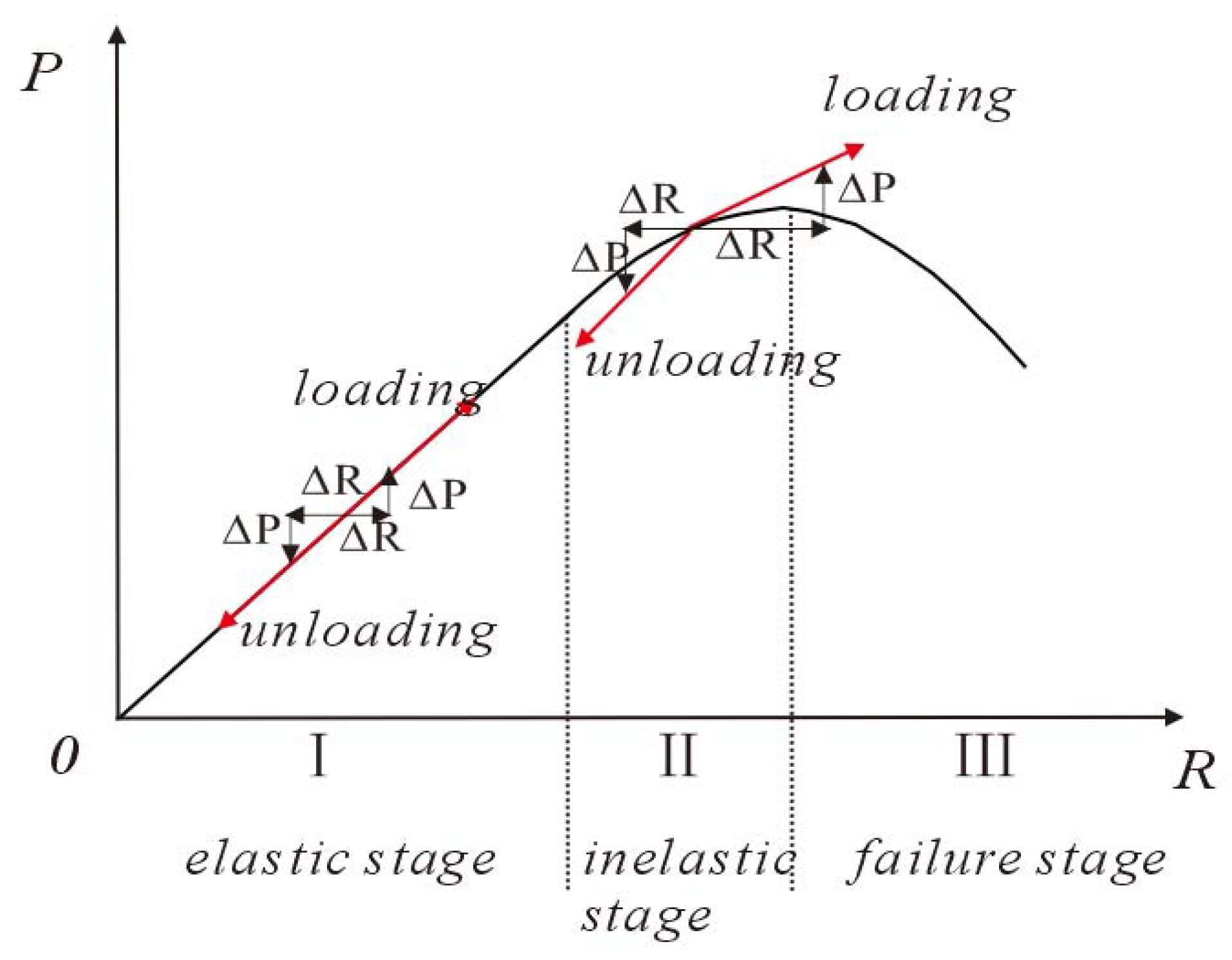
5.1. Relationship between Apparent Resistivity and Stress

Zhao et al. [49] investigated the response of apparent resistivity to tensile and compressive stresses under different conditions (e.g., in situ experiments and mining) and found that the apparent resistivity usually decreased under compression (Figure 5a) and increased under tension (Figure 5b). As discussed above, the Atushi–Kalpin Thrust Zone is dominated by N–S compression, with a minor E–W component. Therefore, decreasing apparent resistivity values are expected in the Kalpin Thrust Zone, at a higher rate in the N–S direction relative to the E–W direction. Our observations were consistent with this expectation (Figure 3a,c).
According to the focal mechanism solution obtained from the USGS, the Jiashi Mw 6.0 earthquake on 19 January 2020 was a thrust rupture event. The detailed source model of the main shock was strike = 221°, dip = 20°, rake = 72°, and depth = 14.9 km, respectively (Figure 5c). We projected the location of the Kalpin Apparent Resistivity Observatory onto the focal sphere and found that both observatories were located in the quadrant where the polarity of the first P wave arrival was positive. In other words, the area hosting these stations experienced tension during the process of earthquake preparation (Figure 5c). According to the response of the apparent resistivity to the tensile stress (Figure 5b), the apparent resistivity should increase during the seismogenic period. The distance between the observation station and the epicenter is about 170 km, which is far greater than the earthquake depth, so it is difficult to establish a definite relationship between the earthquake depth and the change in Kalpin Apparent Resistivity. After September 2019, the annual amplitude of apparent resistivity in the E–W direction at Kalpin Observatory increased by ~0.4 Ωm relative to the previous value (Figure 3b).
Based on the stress recorded in the Kalpin Observatory area and the focal mechanism solution, the monotonic decrease in the apparent resistivity recorded in both directions can be attributed to compressive stress. The resistivity increase recorded in the E–W direction preceding the 2020 Mw 6.0 Jiashi Earthquake was assigned to the tensional stress that occurred in the region during the short-term seismogenic stage.

5.2. Spatiotemporal Evolution of LURR in the Seismogenic Region

The state of earthquake preparation during a large earthquake (M > 6.0) is determined by changes in the constitutive relations of the medium in the seismogenic region.
As shown in Figure 6, when a nonlinear system is in the elastic phase, nearly the same responses (e.g., the strain, energy release, and so on) to the loading and unloading are observed, and LURR ≈1.0; whereas when the system is stressed beyond the elastic limit, the system enters the inelastic stage, microcracks occur in the media, the responses become significantly different, and LURR > 1.0. Thus, the LURR value might serve as a useful index to assess the damaged state of the media.
The energy (or the Benioff strain) of the small earthquakes was used for LURR calculation through the following formula:
Y = E i + E i = B i + B i
where, B i denotes the Benioff strain released by the i-th event, E i denotes the energy of the event, and ‘+‘ and ‘−‘ represent, respectively, the loading and unloading periods derived from the change of Coulomb failure stress (CFS) induced by earth tide in tectonically preferred slip direction [35,36,49,50,51,52,53].
We calculated LURR by using the small earthquakes of M < 4.0 in the Southern Tianshan Mountains (38° N~44° N, 72° E~84° E) from 1 January 2016 to 1 February 2020. Figure 7e shows the time series of LURR produced with small earthquakes within a circular region of 150 km radius center at the Kalpin Observatory. In 2016, a high LURR occurred near the epicenter of the Jiashi Mw 6.0 earthquake, whereas no similar phenomenon was present in the Kalpin Apparent Resistivity Observatory region (Figure 7a). In the next three years (until the end of 2018), the high LURR adjacent to the epicenter progressively decreased, whereas only a slight increase was observed around Kalpin. However, in 2019, the LURR around the Kalpin Observatory increased rapidly (Figure 7d). The apparent resistivity values in the E–W direction also increased and the Jiashi Mw 6.0 earthquake occurred during this period. Combining this with Figure 3a, we note that the value of LURR started to increase in early 2019, while the apparent anomaly occurred in September 2019. The difference is possibly caused by sensitivity of different methods. The occurrence rate of small earthquakes during the loading and unloading processes can induce the change of LURR. However, it takes a certain amount of time for the liquid to make these tiny pores well connected and thus significantly change the apparent resistivity.
Therefore, prior to 2019 (Figure 7a–c), continuous stress caused damage to the medium around the epicenter. However, in the area around the Kalpin Apparent Resistivity Observatory located 169 km from the epicenter, the crustal deformation was mainly characterized by elastic deformation. Conversely, 2019 was characterized by inelastic deformation and microdamage that caused the increase in the apparent resistivity observed in the Kalpin Observatory region until the Jiashi Mw 6.0 earthquake occurred.

5.3. Seepage Gas Monitoring

Figure 8 shows a survey line of a geochemical monitoring campaign that was conducted 23 km south of the Kalpin Apparent Resistivity Observatory by the Earthquake Administration Bureau of the Xinjiang Uygur Autonomous Region. This survey line, which traversed the KPT in an almost N–S direction, included 12 monitoring sites at intervals of 10–15 m. Radon and hydrogen monitoring were performed quarterly. Figure 8a shows the concentrations of Rn and H2, respectively, at each point since 2016. As expected, higher concentrations were generally measured at sites p5 to p7, which are closer to the KPT. Using p5 as an example, we analyzed the changes in the seepage gas near the KPT. Figure 8c,e display the concentrations of Rn and H2, respectively, measured at site p5 since 2016. The highest H2 concentration recorded before the Jiashi Mw 6.0 earthquake occurred in September 2019, while the corresponding Rn concentration was subordinate only to that preceding the Jiashi Mw 5.5 earthquake on 4 September 2018. To highlight this anomaly, we employed the seepage gas intensity, which is the ratio of the maximum to the average concentration measured along the survey line. The seepage H2 intensity in September 2019 was 20% higher than the average value (Figure 8f), whereas the Rn intensity was 12.5% higher than the average value (Figure 8d).
Seepage gases such as Rn are useful geochemical indicators [54]. Their concentrations can be elevated mainly through two processes: (1) increased surface area, owing to the formation of new cracks in the rock and (2) pore water flow. Both of these processes can be explained by microscopic damage to rocks [35,55]. Therefore, the enhanced Rn and H2 concentrations measured along the September 2019 survey line in the Kalpin region further support the presence of microdamage in the surrounding medium [56].
Stress will attenuate drastically as it transfers from the epicenter to the Kalpin Apparent Resistivity Observatory. In theory, if the observatory was located close to the epicenter, the results would be more convincing [57]. However, this region is mainly the sparsely populated Gobi Desert, and additional observatories are not available to verify this hypothesis. In addition, the environmental influence on apparent resistivity would be better described if shallow water level data were available. Despite this, a reasonable explanation can be obtained from existing data for the apparent resistivity variations observed at Kalpin, which indicates that the apparent resistivity of Kalpin is very sensitive to earthquakes that occur on the KPT. Further quantitative research is required to verify the sensitivity of the shallow apparent resistivity to seismic stress, which can help capture earthquake precursor information.

6. Conclusions

The Kalpin Apparent Resistivity Observatory is located in the transitional region between compressional and tensional zones. This complex stress environment caused the value of the apparent resistivity to synchronously and monotonically decrease in both the E–W and N–S directions since 2015, and the annual amplitude in the E–W direction has increased since 2019.
N–S compressive stress dominates the Atushi–Kalpin Thrust Zone. This accounted for the decline in the apparent resistivities in the N–S and E–W directions in the Kalpin region since 2015. The rate of decrease in the N–S direction was approximately twice that in the E–W direction. Prior to 2019, no significant LURR values were measured in the Kalpin Apparent Resistivity Observatory region, and the medium was characterized by elastic deformation.
In early 2019, the value of LURR started to rise, indicating that the medium entered the inelastic stage and microcracks appeared inside. The apparent resistivity anomaly and gas seepage that occurred in September 2019 may be due to the continuous crack growth or the tiny pores being connected. Considering that the Kalpin region was under tensional stress during the seismogenic period of the Jiashi Mw 6.0 earthquake, the annual amplitude of the apparent resistivity in the E–W direction since September 2019 surpassed the previous average values.
Variations in the apparent resistivity recorded at the Kalpin Observatory before the Jiashi Mw 6.0 earthquake on 19 January 2020 reflect physical processes in the medium throughout the seismogenic region. The medium underwent a transformation from elastic deformation to a microdamaged state, until the stress triggered the earthquake. Further quantitative research is required to confirm the relationship between shallow apparent resistivity and seismic stress.

Author Contributions

Writing–original draft preparation, Y.W.; LURR computation, C.Y. (Chen Yu); methodology, H.Y.; GPS strain rate analysis, C.Y. (Chong Yue); gas seepage data collecting, D.J.; gas seepage data analysis, Y.M.; monitoring environment analysis, Z.Z.; focal mechanism solution analysis, W.Y. All authors have read and agreed to the published version of the manuscript.

Funding

This research was funded by the Joint Funds of the National Natural Science Foundation of China (No. U2039205), the National Key Research and Development Project of China (No. 2018YFE0109700), and the Spark Program of Earthquake Technology of the CEA (No. XH20070Y).

Institutional Review Board Statement

Not applicable.

Informed Consent Statement

Not applicable.

Data Availability Statement

The apparent resistivity data and the earthquake catalog were provided by China Earthquake Networks Center. Precipitation data were downloaded from http://data.cma.cn/, accessed on 15 May 2021. Data in Figure 4 were derived from the GPS velocity field relative to the Eurasian plate from 2015 to 2019 calculated by China Earthquake Networks Center and Hubei Earthquake Administration. The moment tensors of the Jiashi Mw 6.0 earthquake were obtained from https://earthquake.usgs.gov/earthquakes/eventpage/us60007anp/moment-tensor, accessed on 15 May 2021. The moment tensors of the Jiashi Ms 5.0 earthquake on 4 September 2018 and the Wushi Ms 5.0 earthquakes on 27 October 2019 were obtained from https://earthquake.usgs.gov/earthquakes, accessed on 15 May 2021, and the moment tensors of the Atushi Ms 5.1 earthquake on 4 November 2018 were obtained from https://www.globalcmt.org, accessed on 15 May 2021. Information about Editage is available at www.editage.cn, accessed on 15 May 2021. All websites were last accessed in May 2021.

Acknowledgments

Some of the figures in this article were prepared using the Generic Mapping Tools software.

Conflicts of Interest

The authors declare no conflict of interest.

References

  1. Yamazaki, Y. Electrical conductivity of strained rocks. The first paper. Laboratory experiments on sedimentary rocks. Bull. Earthq. Res. Inst. 1965, 43, 783–802. [Google Scholar]
  2. Yamazaki, Y. Electrical conductivity of strained rocks. The second paper. Further experiments on sedimentary rocks. Bull. Earthq. Res. Inst. 1966, 44, 1553–1570. [Google Scholar]
  3. Yamazaki, Y. Coseismic resistivity steps. Tectonophysics 1974, 22, 159–171. [Google Scholar] [CrossRef]
  4. Yamazaki, Y. Precursory and coseismic resistivity changes. Pure Appl. Geophys. 1975, 113, 219–227. [Google Scholar] [CrossRef]
  5. Brace, W.F.; Orange, A.S. Electrical resistivity changes in saturated rocks during fracture and frictional sliding. J. Geophys. Res. 1968, 74, 1433–1445. [Google Scholar] [CrossRef]
  6. Brace, W.F.; Paulding, B.W.; Scholz, C. Dilatency in the fracture of crystalline rocks. J. Geophys. Res. 1966, 71, 3939–3953. [Google Scholar] [CrossRef]
  7. Brace, W.F. Dilatancy-related electrical resistivity changes in rocks. Pure Appl. Geophys. 1975, 113, 207–217. [Google Scholar] [CrossRef]
  8. Morrow, C.; Brace, W.F. Electrical resistivity changes in tuffs due to stress. J. Geophys. Res. Solid Earth 1981, 86, 2929–2934. [Google Scholar] [CrossRef]
  9. Walsh, J.B.; Brace, W.F. The effect of pressure on porosity and the transport properties of rock. J. Geophys. Res. 1984, 89, 9425–9431. [Google Scholar] [CrossRef]
  10. Thanassoulas, C. Short-Term Earthquake Prediction; H. Dounias & Co.: Athens, Greece, 2007. [Google Scholar]
  11. Madden, T.R.; La Torraca, G.A.; Park, S.K. Electrical conductivity variations around the Palmdale section of the San Andreas Fault Zone. J. Geophys. Res. 1993, 98, 795–808. [Google Scholar] [CrossRef]
  12. Zhao, Y.; Qian, F. Geoelectric precursors to strong earthquakes in China. Tectonophysics 1994, 233, 99–113. [Google Scholar]
  13. Chu, J.J.; Gui, X.; Dai, J.; Marone, C.; Spiegelman, M.W.; Seeber, L.; Armbruster, J.G. Geoelectric signals in China and the earthquake generation process. J. Geophys. Res. 1996, 101, 13869–13882. [Google Scholar] [CrossRef]
  14. Lu, J.; Xie, T.; Li, M.; Wang, Y.L.; Ren, Y.X.; Gao, S.D.; Wang, L.W.; Zhao, J.L. Monitoring shallow resistivity changes prior to the 12 May 2008 M 8.0 Wenchuan earthquake on the Longmen Shan tectonic zone, China. Tectonophysics 2016, 675, 244–257. [Google Scholar] [CrossRef]
  15. Barsukov, O.M. Variations of electric resistivity of mountain rocks connected with tectonic causes. Tectonophysics 1972, 14, 273–277. [Google Scholar] [CrossRef]
  16. Honkura, Y.; Oshiman, N.; Matsushima, M.; Baris, S.; Tunçer, M.K.; Tank, S.B.; Çelik, C.; Çiftçi, E.T. Rapid changes in the electrical state of the 1999 Izmit earthquake rupture zone. Nat. Commun. 2013, 4, 2116. [Google Scholar] [CrossRef] [Green Version]
  17. Hautot, S. Modeling temporal variations of electrical resistivity associated with pore pressure change in a kilometer-scale natural system, Geochem. Geophys. Geosyst. 2005, 6, Q06005. [Google Scholar] [CrossRef] [Green Version]
  18. Sibson, R.H. Implications of fault-valve behaviour for rupture nucleation and recurrence. Tectonophysics 1992, 211, 283–293. [Google Scholar] [CrossRef]
  19. Uyeshima, M. EM monitoring of crustal processes including the use of the Network-MT observations. Surv. Geophys. 2007, 28, 199–237. [Google Scholar] [CrossRef]
  20. Wannamaker, P.E.; Caldwell, T.G.; Jiracek, G.R.; Maris, V.; Hill, G.J.; Ogawa, Y.; Bibby, H.M.; Bennie, S.B.; Heise, W. The fluid and deformation regime of an advancing subduction system; Marlborough, New Zealand. Nature 2009, 460, 733–736. [Google Scholar] [CrossRef]
  21. Zhao, G.; Unsworth, M.; Zhan, Y.; Wang, L.; Chen, X.; Jones, A.; Tang, J.; Xiao, Q.; Wang, J.; Cai, J.; et al. Crustal structure and rheology of the Longmenshan and Wenchuan Mw 7.9 earthquake epicentral area from magnetotelluric data. Geology 2012, 40, 1139–1142. [Google Scholar] [CrossRef]
  22. Qian, F.Y.; Zhao, Y.L.; Yu, M.M.; Wang, Z.X.; Liu, X.W.; Chang, S.M. Geoelectric resistivity anomalies before earthquakes. Sci. Sin. 1983, 26, 326–336. [Google Scholar]
  23. Qian, J.D. Regional study of the anomalous change in apparent resistivity before the Tangshan earthquake (M = 7.8, 1976) in China. Pure Appl. Geophys. 1985, 122, 901–920. [Google Scholar] [CrossRef]
  24. Qian, F.Y.; Zhao, Y.L.; Xu, T.C.; Zhang, H.K. A model of an impending—Earthquake precursor of geoelectricity triggered by tidal forces. Phys. Earth Planet. Inter. 1990, 62, 284–297. [Google Scholar] [CrossRef]
  25. Park, S.K.; Fitterman, D.V. Sensitivity of the telluric monitoring array in parkfield, california, to changes of resistivity. J. Geophys. Res. Atmos. 1990, 951, 15557–15571. [Google Scholar] [CrossRef]
  26. Park, S.K.; Johnston, M.J.S.; Madden, T.R.F.; Morgan, D.; Morrison, H.F. Electromagnetic precursors to earthquakes in the ULF band: A review of observations and mechanisms. Rev. Geophys. 1993, 31, 117–132. [Google Scholar] [CrossRef]
  27. Parkhomenko, E.I.; Bondarenko, A.T. Effect of uniaxial pressure on electric resistivity of rocks. Bull. Acad. Sci. USSR Geophys. Ser. 1960, 2, 326–332. [Google Scholar]
  28. Skagius, K.; Neretnieks, I. Diffusivity measurements and electrical resistivity measurements in rock samples under mechanical Stress. Water Resour. Res. 1986, 22, 570–580. [Google Scholar] [CrossRef]
  29. Jouniaux, L.; Pozzi, J.P.; Brochot, M.; Philippe, C. Resistivity changes induced by triaxial compression in saturated sandstones from Fontainebleau. C R Acad. Sci. 1992, 315, 1493–1499. [Google Scholar]
  30. Jouniaux, L.; Zamora, M.; Reuschlé, T. Electrical conductivity evolution of non-saturated carbonate rocks during deformation up to failure. Geophys. J. Int. 2006, 167, 1017–1026. [Google Scholar] [CrossRef] [Green Version]
  31. Glover, P.W.J.; Gomez, J.B.; Meredith, P.G.; Hayashi, K.; Sammonds, P.R.; Murrel, S.A.F. Damage of saturated rocks undergoing triaxial deformation using complex electrical conductivity measurements: Experimental results. Phys. Chem. Earth 1997, 22, 57–61. [Google Scholar] [CrossRef]
  32. Yu, H.Z.; Cheng, J.; Zhang, X.T.; Zhang, L.P.; Liu, J.; Zhang, Y.X. Multi-Methods combined analysis of future earthquake potential. Pure Appl. Geophys. 2012, 170, 173–183. [Google Scholar] [CrossRef]
  33. Ma, J.; Ma, S.H.; Liu, L.Q. The stages of anomalies before an earthquake and the characteristics of their spatial distribution. Seismol. Geol. 1995, 17, 363–371, (In Chinese with an English abstract). [Google Scholar]
  34. Scholz, C.H.; Sykes, L.R.; Aggrawal, Y.P. Earthquake prediction: A physical basis. Science 1973, 181, 803–809. [Google Scholar] [CrossRef] [PubMed]
  35. Yin, X.C.; Chen, X.Z.; Song, Z.P.; Yin, C. A new approach to earthquake prediction: The Load/Upload Response Ratio (LURR) theory. Pure Appl. Geophys. 1995, 145, 701–715. [Google Scholar] [CrossRef]
  36. Yin, X.C.; Wang, Y.C.; Peng, K.Y.; Bai, Y.L.; Wang, H.T. Development of a new approach to earthquake prediction: Load/Unload Response Ratio (Lurr) theory. Pure Appl. Geophys. 2000, 157, 2365–2383. [Google Scholar]
  37. Yin, X.C.; YU, H.Z.; Kukshenko, V.; Xu, Z.Y.; Wu, Z.S.; Li, M.; Peng, K.Y.; Elizarov, S.; Li, Q. Load-Unload Response ratio (LURR), Accelerating Energy release (AER) and State Vector evolution as precursors to failure of rock specimens. Pure Appl. Geophys. 2004, 161, 2405–2436. [Google Scholar] [CrossRef] [Green Version]
  38. Zhang, Y.X.; Yin, X.C.; Peng, K.Y. Spatial and Temporal Variation of LURR and its Implication for the Tendency of Earthquake Occurrence in Southern California. Pure Appl. Geophys. 2004, 161, 2359–2367. [Google Scholar] [CrossRef] [Green Version]
  39. Gan, W.; Prescott, W. Crustal deformation rates in the central and eastern U. S. Inferred from GPS. Geophys. Res. Lett. 2001, 28, 3733–3736. [Google Scholar] [CrossRef]
  40. Wu, W.W. Insight into the Characteristics of GPS Time Series in North China; Institute of Earthquake Forecasting, CEA: Beijing, China, 2014; pp. 46–47. [Google Scholar]
  41. Xu, X.W.; Zhang, X.K.; Ran, Y.K.; Cui, X.F.; Ma, W.T.; Shen, J.; Yang, X.; Han, Z.J.; Song, F.M.; Zhang, L.F. The preliminary study on Seismotectics of the 2003 AD Bachu-Jiash Earthquake (Ms6.8), southern Tian Shan. Seismol. Geol. 2006, 28, 161–178, (In Chinese with an English abstract). [Google Scholar]
  42. Scharer, K.M.; Burbank, D.W.; Chen, J.; Weldon, R.J.; Rubin, C.; Zhao, R.; Shen, J. Detachment folding in the Southwestern TianShan Tarim foreland, China: Shortening estimates and rates. J. Struct. Geol. 2004, 26, 2119–2137. [Google Scholar] [CrossRef]
  43. Yang, X.P.; Deng, Q.D.; Zhang, P.Z. crustal shortening of major nappe structures on the front margins of the Tianshan. Seismol. Geol. 2008, 30, 111–131. [Google Scholar]
  44. Allen, M.; Vincent, S.; Wheeler, P.J. Late Cenozoic tectonics of the Kepingtage thrust zone: Interactions of the Tien Shan and Tarim basin, northwest China. Tectonics 1999, 18, 639–654. [Google Scholar] [CrossRef]
  45. Li, A.; Ran, Y.; Xu, L.; Liu, H. Paleoseismic study of the east Kalpintage fault in southwest Tianshan based on deformation of alluvial fans and 10Be dating. Nat. Hazards 2013, 68, 1075–1087. [Google Scholar] [CrossRef]
  46. Li, A.; Ran, F.Y.; Gomez, J.A.T.; Jobe, H.; Xu, L. Segmentation of the Kepingtage thrust fault based on paleoearth-quake ruptures, southwestern Tianshan, China. Nat. Hazards 2020, 103, 1385–1406. [Google Scholar] [CrossRef]
  47. Yao, Y.; Wen, S.; Li, T.; Wang, C. The 2020 Mw6.0 Jiashi Earthquake: A Fold Earthquake Event in the Southern Tian Shan, Northwest China. Seismol. Res. Lett. 2020, 92, 859–869. [Google Scholar] [CrossRef]
  48. Lu, J.; Xue, S.; Qian, F.; Zhao, Y.; Guan, H.; Mao, X.; Ruan, A.; Yu, S.; Xiao, W. Unexpected changes in resistivity monitoring for earthquakes of the Longmen Shan in Sichuan, China, with a fixed Schlumberger sounding array. Phys. Earth Planet. Inter. 2004, 145, 87–97. [Google Scholar] [CrossRef]
  49. Wang, M.; Shen, Z.K. Present-day crustal deformation of continental China derived from GPS and its tectonic implications. J. Geophys. Res. Solid Earth 2020, 25, e2019JB018774. [Google Scholar] [CrossRef] [Green Version]
  50. Li, G.R.; Sulitan, Y.S.; Ailixiati, Y.S.; Liu, D.Q.; Buaijier, K.; Zhao, L.; Ding, Y. Characteristics of GNSS anomalies before and after Jiashi Ms6.4 earthquake in Xinjiang on January 19th, 2020. Inland Earthq. 2020, 34, 70–78, (In Chinese with an English abstract). [Google Scholar]
  51. Zhao, Y.L.; Qian, F.Y.; Yang, T.C.; Liu, J.Y. The experiments on electric resistivity in situ. Acta Seismol. Sin. 1983, 5, 217–225, (In Chinese with an English abstract). [Google Scholar]
  52. Yu, H.Z.; Shen, Z.K.; Wan, Y.G.; Zhu, Q.Y.; Yin, X.C. Increasing critical sensitivity of the load/unload response ratio before large earthquakes with identified stress accumulation pattern. Tectonophysics 2006, 428, 87–94. [Google Scholar] [CrossRef]
  53. Yu, H.Z.; Zhu, Q.Y. A probabilistic approach for earthquake potential evaluation based on the load/unload response ratio method. Concurr. Comput. Pract. Exp. 2010, 22, 1520–1533. [Google Scholar] [CrossRef]
  54. Yu, H.Z.; Zhou, F.R.; Cheng, J.; Wan, Y.G. The sensitivity of load/unload response ratio and critical region selection before large earthquakes. Pure Appl. Geophys. 2015, 172, 173–183. [Google Scholar] [CrossRef]
  55. Yu, H.Z.; Yu, C.; Ma, Z.X.T.; Zhang, H.; Yao, Q.; Zhu, Q.Y. Temporal and spatial evolution of Load/Unload Response Ratio before the M7.0 Jiuzhaigou earthquake of Aug. 8, 2017 in Sichuan Province. Pure Appl. Geophys. 2020, 177, 321–331. [Google Scholar] [CrossRef]
  56. Walia, V.; Virk, H.S.; Bajwa, B.S. Radon precursory signals for some earthquakes of magnitude > 5 Occurred in N-W Himalaya: An overview. Pure Appl. Geophys. 2006, 163, 711–721. [Google Scholar] [CrossRef]
  57. Mjachkin, V.I.; Brace, W.F.; Sobolev, G.A.; dieterich, J.H. Two models for earthquake forerunners. Pure Appl. Geophys. 1975, 113, 169–182. [Google Scholar] [CrossRef]
Figure 1. Main faults in the Atushi–Kalpin Thrust Zone and the locations of geophysical observatories. Red lines indicate active faults, including the Kalpintag Thrust Fault (KPT), Aozigertawu Thrust Fault (AZT), Toksanatanengbayler Thrust Fault (TST), Kekebuke Sanshan Thrust Fault (KST), Aoyibulake Thrust Fault (AYT), Tataiertage Thrust Fault (TAT), and Yimugantawu Thrust Fault (YMT) [39]. The red triangle indicates the location of the Kalpin Apparent Resistivity Observatory, the yellow square indicates the location of the Kalpin Meteorological Observatory, and the dashed blue lines denote the crustal deformation baselines. Black dots indicate GPS observation sites and LL’ represents the geochemical survey line.
Atmosphere 12 01420 g001
Figure 2. Illustration of the (a) Schlumberger array employed at the Kalpin Geoelectric Resistivity Observatory and the observation environment (the yellow area is part of the Gobi Desert, while the green area represents farmland) and (b) the electrode layout employed in the resistivity measurements.
Atmosphere 12 01420 g002
Figure 3. Plots of the apparent resistivity recorded at the Kalpin Observatory: (a) the blue curve is the E–W daily average of apparent resistivity, and the green curve is the temporal curve of LURR mean value within 150 km around Kalpin observatory, (b) annual variation of the E-W direction, (c) N–S daily average, (d) annual variation of the N-S direction, and (e) precipitation data for 2015–2019 (from the Kalpin Meteorological Station). Blue columns indicate daily precipitation and red dots indicate the monthly precipitation averages. ①, ②, ③, and ④ represent the Jiashi Ms 5.5 earthquake on 4 September 2018, the Atushi Ms 5.1 earthquake on 4 November 2018, the Wushi Ms 5.0 earthquake on 27 October 2019, and the Jiashi Mw 6.0 earthquake on 19 January 2020.
Atmosphere 12 01420 g003
Figure 4. (a) Continuum strain field of the Atushi–Kalpin Thrust Zone derived from interpolated GPS velocities. The dilatation rate is in color, while the principal strain rates are denoted as vector pairs. (b) Strain plot for the Kalpin Apparent Resistivity Observatory, showing values for the N–S and E–W components.
Atmosphere 12 01420 g004
Figure 5. Plots of the (a) resistivity variations with pressure loading (compression) and unloading (dilatancy) and (b) resistivity variations with tension loading (dilatancy) and unloading (compression) [14,49]. And (c) focal sphere of the Jiashi Mw 6.0 earthquake on 19 January 2020. The yellow triangle indicates the location of the Kalpin Apparent Resistivity Observatory.
Atmosphere 12 01420 g005
Figure 6. Schematic diagram of the constitutive relation of rock. P and R represent, respectively, the load and response. At stage I, the responses ( Δ R ) to the small changes of Δ P in the loading and unloading are almost the same, while at the stage II, the response to the loading is significantly greater than the unloading, and the stage Ⅲ is characterized with macroscopic damage.
Atmosphere 12 01420 g006
Figure 7. Spatiotemporal evolution of the load/unload response ratio (LURR) in the Atushi–Kalpin Thrust Zone from 1 January 2016 to 31 December 2019 (ad); (e) is the temporal curve of LURR mean value within 150 km around Kalpin observatory. The red star indicates the epicenter of the Jiashi Mw 6.0 earthquake and the pink triangle indicates the location of the Kalpin Apparent Resistivity Observatory.
Atmosphere 12 01420 g007
Figure 8. Location of the geochemical survey line (LL’’) in the Kalpin region (a), where (b) shows the radon and hydrogen concentrations, respectively, measured at each monitoring site. Axis of abscissas in (b) indicates the distance between the monitoring point andp1. (c,e) show the radon and hydrogen concentrations measured at monitoring site p5, respectively, and (d,f) show the radon and hydrogen intensities, respectively.
Atmosphere 12 01420 g008
Publisher’s Note: MDPI stays neutral with regard to jurisdictional claims in published maps and institutional affiliations.

