Possible Linkages of Hydrological Variables to Ocean–Atmosphere Signals and Sunspot Activity in the Upstream Yangtze River Basin

Abstract

Profiling the hydrological response of watershed precipitation and streamflow to large-scale circulation patterns and astronomical factors provides novel information into the scientific management and prediction of regional water resources. Possible contacts of El Niño–Southern Oscillation (ENSO), Pacific Decadal Oscillation (PDO), sunspot activity to precipitation and streamflow in the upper Yangtze River basin (UYRB) were investigated in this work. Monthly precipitation and streamflow were utilized as well as contemporaneous same-scale teleconnections time series spanning a total of 70 years from 1951 to 2020 in precipitation and 121 years from 1900 to 2020 in streamflow. The principal component analysis (PCA) method was applied so as to characterize the dominant variability patterns over UYRB precipitation time series, with the temporal variability of first two modes explaining more than 80% of total variance. Long-term evolutionary pattern and periodic variation characteristics of precipitation and streamflow are explored by applying continuous wavelet transform (CWT), cross-wavelet transform (XWT) and wavelet coherence (WTC), analyzing multi-scale correlation between hydrological variables and teleconnections in the time-frequency domain. The results manifest that ENSO exhibits multiple interannual period resonance with precipitation and streamflow, while correlations are unstable in time and phase. PDO and sunspot effects on precipitation and streamflow at interannual scales vary with time-frequency domains, yet significant differences are exhibited in their effects at interdecadal scales. PDO exhibits a steady negative correlation with streamflow on interdecadal scales of approximately 10 years, while the effect of sunspot on streamflow exhibits extremely steady positive correlation on longer interdecadal scales of approximately 36 years. Analysis reveals that both PDO and sunspot have significantly stronger effects on streamflow variability than precipitation, which might be associated with the high spatiotemporal variability of precipitation.

1. Introduction

Global climate change has influenced global and regional hydrological cycles [1]. The effect of large-scale climate effects in modulating water cycle events provides the key for anticipating variation of hydrological factors [2]. Comprehending the variability of hydrological variables such as precipitation and streamflow is fundamental to understanding water cycle dynamics [3,4,5], while such variability has been indicated to be associated with climate change effects and large-scale climate anomalies [3,6]. Hence, understanding the telecorrelated relationship between different climate indices and local hydrological variables can provide new guidance for improving water system models and optimizing water resources management in specific regions [7].

Ocean–atmosphere interactions tend to be closely related to hydrological variables and hence provide valuable information for hydrological forecasting [8]. As the main components of hydrological cycle, precipitation [9] and streamflow [1] are influenced by complex ocean–atmosphere interactions. Oceanic–atmospheric phenomena of different timescales might simultaneously affect the precipitation and streamflow in several watershed around the world [3]. El Niño–Southern Oscillation (ENSO) is the outcome of oceanic and atmospheric interactions at macroscopic spatial scales that is treated as the strongest interannual signal of climatic changes [10,11]. ENSO dominates tropical Pacific climate variability on interseasonal to interannual timescales, which is the primary source of predictability of global climate variability at these timescales [12,13]. ENSO has been recognized as the dominating climate modulator of precipitation on global scale, which further affects streamflow and other hydrologic cycle variables [2,11]. Based on teleconnections affecting coupled ocean atmosphere and land systems, ENSO events are closely linked to the patterns of flood and drought all around the world [11], which strongly affect local- and regional-scale climates [1,14]. Pacific Decadal Oscillation (PDO) is a periodic pattern of oceanic and atmospheric climate change centered on mid-latitude Pacific basins, manifest as the predominant empirical orthogonal function (EOF) of sea surface temperature (SST) variability in the Pacific basin poleward of 20° N [15]. Previous analysis has shown that PDO influences precipitation and streamflow as much as ENSO [16], and the effects of PDO and ENSO appear to be additive when both are in the same phase [17,18]. Hydrological time series have been indicated to exist climatic variability and to partially coincide with known climate cycles such as ENSO and PDO [19]. Therefore, relevant information of ENSO and PDO would cause improvements in precipitation and streamflow predictions, thereby mitigating floods and droughts in the Pacific region and elsewhere [19,20]. Since the influences of ENSO and PDO have significant temporal variability [17,21], the value of using climate indices such as ENSO or PDO in water resource predictions depends on understanding of the local relationship between these indices and hydrological factors on time [17].

Solar irradiation is the dominant driving force of the Earth’s climate system [22]. The fluctuations and distribution of hydrological signals are highly correlated with geophysical system [23]. Previous studies have confirmed that the variability of solar activity influences global climate on various timescales [22,24,25], with negative anomalies of SST in equatorial Pacific during high solar activity years [26]. Sea temperature varies in-phase with an 11-year solar activity cycle [27,28,29], which could force the Pacific decadal variability [22]. Solar activity maxima and minima refer to periods of maximum and minimum sunspot counts, with a solar cycle spanning from one sunspot minimum to the next [27]; hence, sunspot number is a possible indicator of solar activity associated with climate. Gaining a comprehensive understanding of the effects of oceanic–atmospheric climate anomalies and solar activity on temporal variability of precipitation and streamflow in specific watersheds is of great significance for hydrological simulation, climate change and risk management as well as for addressing water-resource-related issues [3,30,31]. Due to its proximity to the Pacific Ocean, the Yangtze River basin is prominently sensitive to such climatic phenomena as El Niño–Southern Oscillation (ENSO) [32,33,34,35,36] and Pacific Decade Oscillation (PDO) [33,35,37,38], which have significant implications for forecasting water resources and climate conditions. In recent years, studies in the Yangtze River basin and its tributaries have made significant advances in the influence of large-scale teleconnection patterns on hydrological variability [33,35,37,39,40,41,42,43,44,45], while the temporal persistence of these relationships is not yet wholly understood. Additionally, as global climate conditions have changed, the intensity and frequency of ENSO events have increased since the late 1970s [26], and ocean–atmosphere forcing has become one of the most potential sources of global natural variability [1]; however, the influence of large-scale climate variability on precipitation and streamflow in the UYRB has rarely been examined.

To this end, the main objective of this study is to analyze multi-timescale correlations of tropical and mid-latitude Pacific climatic oscillations and sunspot activity with hydrological factors on a monthly timescale by utlizing continuous wavelet transform (CWT), cross-wavelet transform (XWT) and wavelet coherence (WTC), and to investigate the periodic evolution of precipitation and streamflow in the upper Yangtze River basin and their possible link to telecorrelation factors. Tropical Pacific climate forcing is represented by oceanic atmospheric ENSO, while mid-latitude Pacific oscillation is represented by oceanic atmospheric climate pattern PDO. In addition, the interdecadal variability of streamflow possibly associated with the influences of PDO and sunspot activity was studied. Multi-timescale correlation analysis contributes to understanding relations of hydrological response with climate forcing, providing novel information for enabling regional water resources management. 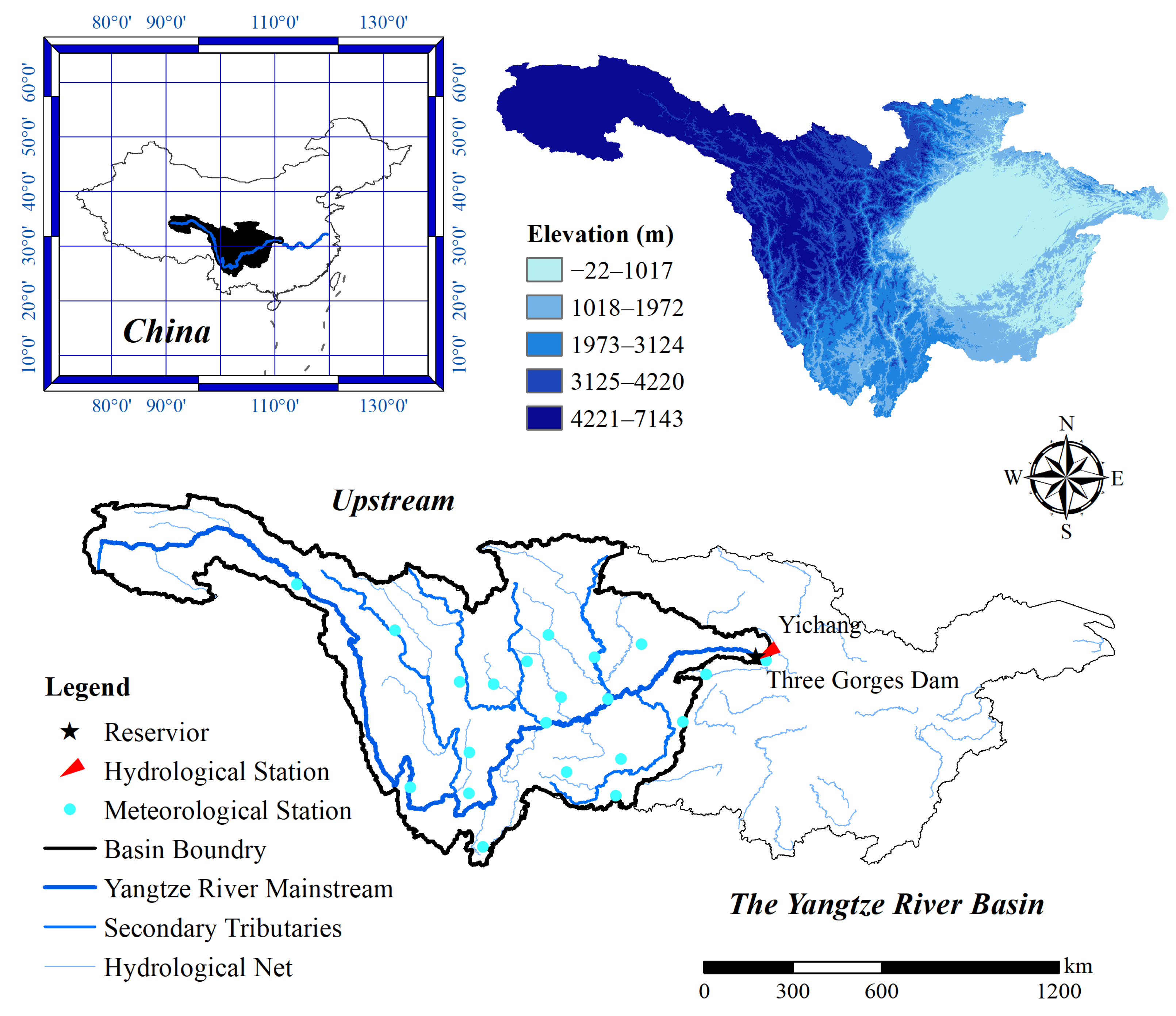The contents of this paper are assigned as follows: Section 2 describes the study area and presents data sources; Section 3 introduces the main methodology; Section 4 provides study results; Section 5 and Section 6 present discussion and conclusions, respectively.

2. Materials

2.1. Study Area

With a total length of more than 6300 km [46], the Yangtze River is the longest river in China and the third-longest river in the world, second merely to the Nile and the Amazon river [5,43]. The upper Yangtze River is 4511 km in length, originating in the hinterland of Qinghai–Tibetan Plateau and ending at Yichang, Hubei Province. The upper Yangtze River basin (UYRB) is located between 90°13′–111°30′ E and 24°37′–35°54′ N, with geographical location showing in Figure 1.

The elevation of whole basin ranges from −22–7143 m, annual precipitation ranges from 739–1036 mm (from 1951 to 2020) and annual streamflow is approximately 440 billion m³ (from 1900–2020). Influenced by the East Asian monsoon, South Asian monsoon and unique topography of Qinghai–Tibet Plateau, the meteorological and hydrological characteristics have significant seasonal variations [47]. The intra-annual distribution of precipitation and streamflow is uneven, with 75% of precipitation and 70% of streamflow throughout the year concentrated during the flood season from May to October, when rainstorms and floods occur frequently, while a smaller proportion of precipitation and streamflow occurs during the non-flood season. The upper reaches of the Yangtze River can be classified into five main sub-basins of Jinsha River, Min-tuo River, Jialing River, Wu River and the upper Yangtze River mainstream area, accounting for 32.8%, 22.7%, 16.1%, 11.3% and 17.0% of total upstream flow, respectively. The Yichang hydrographic station [36,43], the export control station of the upstream Yangtze River, controls a watershed area of 1,005,501 km², accounting for 55.8% of the Yangtze River basin area [48], including the Three Gorges Reservoir and Gezhouba Reservoir, located 44 km and 6 km upstream of the Yichang section, respectively [48]. Hydrological variability in the upstream Yangtze River affects water fluctuations and power generation downstream, thus insights from this study are useful for water resources planning and management in the Yangtze River basin.

2.2. Data Sources

2.2.1. Precipitation and Streamflow

Relationships between teleconnections and hydrological variables are characterized by temporal and spatial variability that cannot be adequately evaluated without long-term hydrological and meteorological records [17,49]. Therefore, the longest and most complete record possible should be used when searching for secular trends in regions that are equally affected by low-frequency climate cycles (e.g., PDO) [17]. Twenty-one national meteorological stations in the UYRB with a 70-year span time series from January 1951 to December 2020 was utlized, and the monthly precipitation data were derived from the National Climate Center, China Meteorological Administration http://cmdp.ncc-cma.net/cn/index.htm, accessed on 10 August 2021).

The controlling hydrological station for upper reaches of the Yangtze River export, the Yichang hydrological station, with a total streamflow time series of 121 years spanning from January 1900 to December 2020, was used in the current study. The monthly mean streamflow data were derived from the Local Hydrographic Bureau, which has been effectively quality-controlled and compiled.

2.2.2. ENSO

With recurring periodicities of 2–7 years, ENSO describes the movement of equatorial Pacific waters associated with sea surface temperature variations and the fluctuations in atmospheric pressure patterns in the tropical Indian and Pacific Oceans associated with the Pacific trade winds [50,51]. The Nino3.4 SST index based on regional mean sea surface temperature (SST) anomalies and Southern Oscillation index based on mean sea level pressure (SLP) differences were used to characterize ENSO intensity in this study [52]. The Nino3.4 index is defined as mean monthly SST anomalies over the Nino3.4 region (5° S 5° N, 170° W 120° W) of equatorial Pacific Ocean [12,17], derived from IRI/LDEO Climate Data Library (http://iridl.ldeo.columbia.edu/SOURCES/.Indices/.nino/, accessed on 6 August 2021). The Southern Oscillation Index (SOI) gives an indication of the development and intensity of El Niño or La Niña events in the Pacific Ocean region [13], derived from the Bureau of Meteorology, Australian Government (http://www.bom.gov.au/climate/enso/soi/, accessed on 6 August 2021).

2.2.3. PDO

Explained as the secular oceanic fluctuation of the Pacific [50], PDO is a large-scale climate pattern of SST fluctuation between cool SST anomalies in the central-eastern North Pacific Ocean, and warm SST anomalies along the central-western coast of North America [15,53]. PDO waxes and wanes approximately every 20–30 years, with longer cycles compared to ENSO, its periodicity recurring over decadal (around 15–25-year) to multidecadal (around 50–70-year) cycles [15,50,54]. The PDO index is defined as the dominant principal component of North Pacific monthly SST variability, i.e., the time factor of the first mode after EOF decomposition in North Pacific (20°–70° N, 110° E–100° W) [52] monthly time series was derived from the National Centers for Environmental Information, National Oceanic and Atmospheric Administration (https://www.ncdc.noaa.gov/teleconnections/pdo/, accessed on 6 August 2021).

2.2.4. Sunspot

Solar activity has an average cycle with a duration of approximately 11 years [22,25,27]. The solar activity data, i.e., sunspot number (SSN), was obtained from the Royal Observatory of Belgium, Brussels (https://wwwbis.sidc.be/silso/datafiles, accessed on 7 August 2021), which is calculated from Equation (1) [27]:

$$R_{SSN}=k\left(10g+s\right)$$

(1)

where R is the sunspot number, also referred to as $SSN$; k is the observatory scaling factor; g is the number of sunspot groups; and s is the number of individual sunspots.

Figure 2 depicts monthly time series of four indexes with a time span from January 1900 to December 2020 used in this study. The black dotted line in the figure is the original time series showing that indexes are nonststionary time series with periodical fluctuation characteristics. To reduce the interference of intra-annual oscillations and seasonal fluctuations, low-pass filtering was applied to original series by using 13-month sliding average to visualize the interannual and interdecadal variability features of factor series, which are given as red-blue envelopes in Figure 2.

3. Methodology

3.1. Principal Component Analysis

Principal component analysis (PCA) is a technique for reducing the dimensionality of large datasets, increasing interpretability while at the same time minimizing information loss [55]. PCA is frequently used in rainfall data for its dimensionality reduction [3,56] to obtain an uncorrelated orthogonal basis set derived from a climatic dataset, which is a multivariate statistical technique that is widely applied to pattern recognition in climatology time series of spatial fields [57]. One of the main purposes of PCA is to reduce the number of series to be studied while preserving as much variability (i.e., statistical information) as possible contained in the original set of variables in order to understand and interpret the structure of the data [58]. Often useful insights into multivariate data arise from the interpretation of these transformations [59]. PCA does so by creating new uncorrelated variables that successively maximize variance, and such new variables are linear functions of those in the original dataset, i.e., the principal components (PCs), hence being reduced to solving an eigenvalue or eigenvector problem [55]. Each PC is characterized by its variance, also referred to as eigenvalue, which is a measurement of its importance in explaining variation [57].

In the present research, PCA was applied in order to characterize the dominant variability patterns over monthly UYRB precipitation time series from 21 meteorological stations with a time span of January 1951 to December 2020. The emphasis in PCA is almost always on the first few PCs, and it is common practice to use some predefined percentage of total variance explained to decide how many PCs should be retained (common for 70% of total variability). Among such situations, the percentage of total variance accounted for is a fundamental tool to assess the quality of these low-dimensional graphical representations of the dataset [55]. PCA has choices associated with its use, for instance how many PCs to retain [60]. In this work, the Kaiser–Meyer–Olkin (KMO) was calculated as a value of 0.874, which is an index evaluating multicollinearity among stations [3]. The Bartlett’s sphericity test [61] carried out on the correlation matrix shows a calculated ${\chi }^2$ = 1621.861, greater than the critical value ${\chi }^2$ = 146.6 (p-value = 0.05), and gained a p-value < 0.001, manifesting that PCA can achieve a significant reduction of the dimensionality of the original data set. The two components of those eigenvalues greater than 1 were retained, with the first and second components’ variances accounting for 73.303% and 6.953% of the initial data variance in precipitation series, respectively, and the cumulative variance explained by 80.256%, which is efficient to characterize the fluctuation of precipitation series in the UYRB.

3.2. Continuous Wavelet Transform

Continuous wavelet transform (CWT) can be used for analyzing time series containing nonstationary power at many different frequencies, with clearly describing the dominant patterns of variation [46,62] and analyzing the localized intermittent oscillations in hydrological time series [51,63]. Studies have shown that CWT is appropriate for analyzing time series with non-normal distribution [64], which are frequently found in nonstationary parameters, for instance such hydrological variables as precipitation and streamflow [51]. For the sake of determining the predominant mode of variability, CWT was performed on precipitation and streamflow series in the UYRB.

CWT was applied to decompose the time series into all possible continuous scales and generate a two-dimensional wavelet spectrum to reveal the temporal evolution and variability of each periodicity [50,64]. With the purpose of applying wavelet as a bandpass filter to time series, for discrete sequence ($x_n,n=1,\cdots ,N$), the CWT with uniform interval of $\delta t$ can be defined as the convolution of $x_n$ with scaled and normalized wavelet [64,65]:

$$W_n^X\left(s\right)=\sqrt{\frac{\delta t}{s}}\sum _{n^{\prime }=1}^N{x}_{n^{\prime }}{\psi }_0\left[\left(n^{\prime }-n\right)\frac{\delta t}{s}\right]$$

(2)

where $\sqrt{\frac{\delta t}{s}}$ denotes the normalization factor that results in $\psi$ having unit energy. Wavelet power is defined as ${\left|W_n^X\left(s\right)\right|}^2$.

Due to dealing with finite-length time series, the artificial edge effects exist [64]. The cone of influence (COI) is the region of wavelet spectrum in which edge effects cannot be ignored, which is deemed as the area in which wavelet power caused by a discontinuity at edge has dropped to $e^{-2}$ of the value at edge [64,65]. The significance levels of the wavelet spectrum were analyzed in a background of red noise, the appropriate stochastic background spectrum for numerous geophysical phenomena and which can be modeled as a univariate lag1 autoregressive process [65]. Significance at the 5% level is equivalent to pass the 95% confidence level [24]; hence, the significance level of p < 0.05 was used to evaluate the statistical significance of results.

The Morlet wavelet has been proven as the most appropriate wavelet function to be used for analyzing geophysical signals [51,65] since that adequately describes the shape of hydrological-type data and a better frequency resolution than other wavelets such as the Mexican Hat and Paul and Daubechies wavelets [50]. Assume that a time series, $x_n$, has equal time intervals $\delta t$ and $n=0\cdots N-1$, and a wavelet function, ${\psi }_0\left(\eta \right)$, depending on parameter $\eta$ [65]. Consisting of a Gaussian modulated plane wave, the Morlet wavelet is a nonorthogonal complex function, which can be defined as [64,65,66]:

$${\psi }_0\left(\eta \right)={\pi }^{-1/\phantom{-14}4}{e}^{i{\omega }_0\eta }{e}^{-\frac{1}{2}{\eta }^2}$$

(3)

where ${\omega }_0=6$ is dimensionless frequency, providing a good balance between time and frequency localization, and $\eta$ is the dimensionless time parameter.

3.3. Cross-Wavelet Transform and Wavelet Coherence

Cross-wavelet transform (XWT) and wavelet coherence (WTC) are powerful methods for testing proposed linkages between two time series at multiple timescales [46,64]. From the CWTs of two time series, XWT and WTC can be calculated, where XWT exposes regions with high common power and further reveals information about phase relationship, while WTC can be thought of as local correlations between two time series in time frequency space [39,51,64]. Hence, XWT identifies high common power, WTC unveils locally phase-locked behavior [64] and the relative phase between two time series could also be identified from XWT or WTC [39,65].

Given two time series X and Y, with wavelet transforms $W_n^X\left(s\right)$ and $W_n^Y\left(s\right)$, the cross-wavelet spectrum, which shows the covariance of two time series, can be defined as [65]:

$$W_n^{XY}\left(s\right)=W_n^X\left(s\right)W_n^{Y\ast }\left(s\right)$$

(4)

where ∗ indicates the complex conjugate, $\left|W_n^{XY}\left(s\right)\right|$ can be defined as cross-wavelet power and the complex argument $W_n^{XY}\left(s\right)$ can be interpreted as local relative phase between $x_n$ and $y_n$ in time frequency space [64,65].

WTC quantifies the correlation and reveals regions in time frequency space where the two time series covary but do not necessarily have high power [66,67], and the wavelet coherence of two time series can be defined as [65]:

$$R_n^2\left(s\right)=\frac{{\left|S\left(s^{-1}{W}_n^{XY}\left(s\right)\right)\right|}^2}{S\left(s^{-1}{\left|W_n^X\left(s\right)\right|}^2\right)·S\left(s^{-1}{\left|W_n^Y\left(s\right)\right|}^2\right)}$$

(5)

where S is a smoothing operator defined by the wavelet type used. $R^2$ takes a value between $\left(0,1\right)$: 0 indicates no correlation between two time series, while 1 indicates two time series that are perfectly correlated.

In the present research, the Monte Carlo approach was adopted to calculate the statistical significance of the wavelet coherence [2]. The circular mean of phase angle over regions with higher than 5% statistical significance that are outside COI can be utlized to quantify the phase relationship [64]; statistically significant covariance was determined against red noise background [65,68].

4. Results

4.1. Temporal Patterns of Hydrological Variables

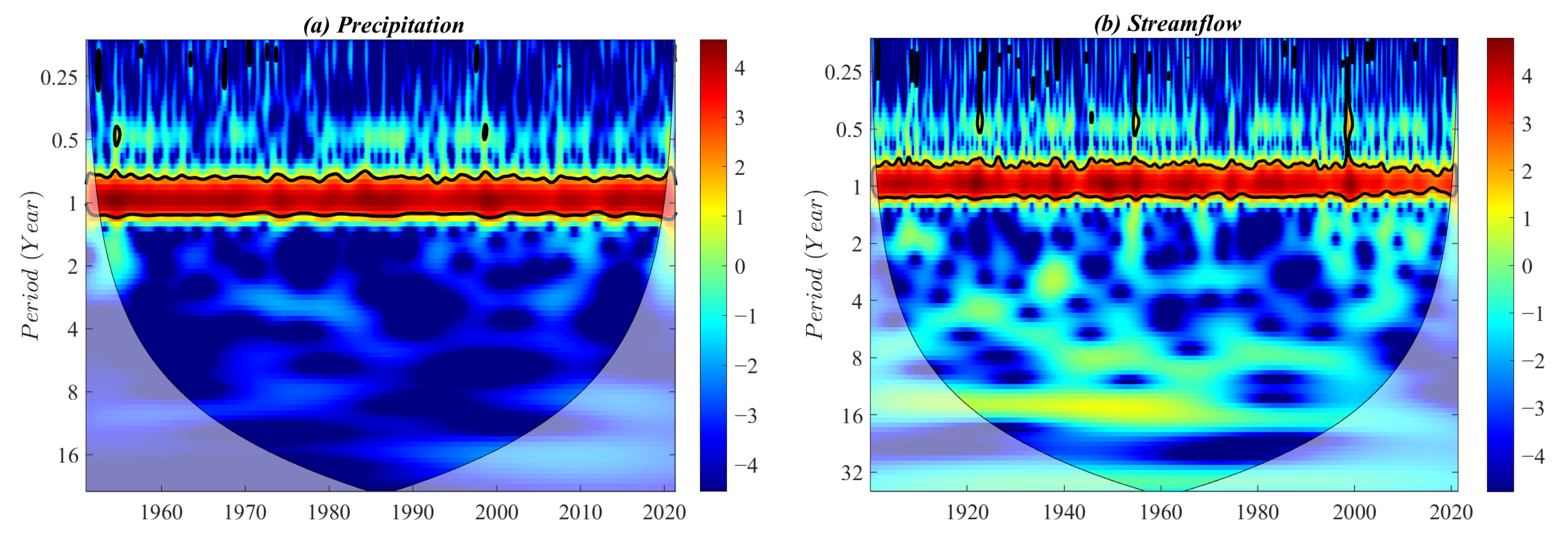
The evolution of hydrological variables has a significant characteristic of multiple timescales. Multiple timescales of hydrological variable series, such as precipitation and streamflow, are generally manifested as small time-scale variation cycles nested in large-scale variation cycles, i.e., multi-level timescale structures and localized variation characteristics exist in precipitation and streamflow variability within the time domain. Continuous wavelet transform was applied to analyze the multi-timescale oscillations and periodic fluctuation characteristics of monthly precipitation and streamflow series in the UYRB, with the continuous wavelet power spectrum given in Figure 3. Thin solid lines in the figure denote the cone of influence (COI) with wavelet boundary effects, where the edge effects may distort calculation results [64]. Thick black contours denote 5% significance levels, i.e., they passed the red noise test with 95% confidence levels [65]. The color denotes the strength of wavelet power [66].

Continuous wavelet power spectrums indicate that precipitation and streamflow series have highly significant 0.8–1.2-year interannual oscillation, which exhibit continuous annual periodicity throughout the study time domain. Moreover, the precipitation series shows intermittent 1–4-month cycle during 1950 to 1975; and the streamflow series shows frequent 1–6-month significant cycle over the whole study time (January 1900 to December 2020), yet time of duration is short and cyclic oscillations are unstable.

Furthermore, except for an extremely significant annual cycle of about 1-year, precipitation and streamflow series do not show significant cyclical variation on longer interannual and interdecadal scales. In order to eliminate the disturbance of annual oscillation and seasonal fluctuation, Morlet complex wavelet transform was utilized to analyze the continuous multi-timescale characteristics of annual precipitation and annual streamflow evolution, to determine the relative intensity of fluctuation and the main timescales of variability on interannual and interdecadal scales, i.e., the main cycles.

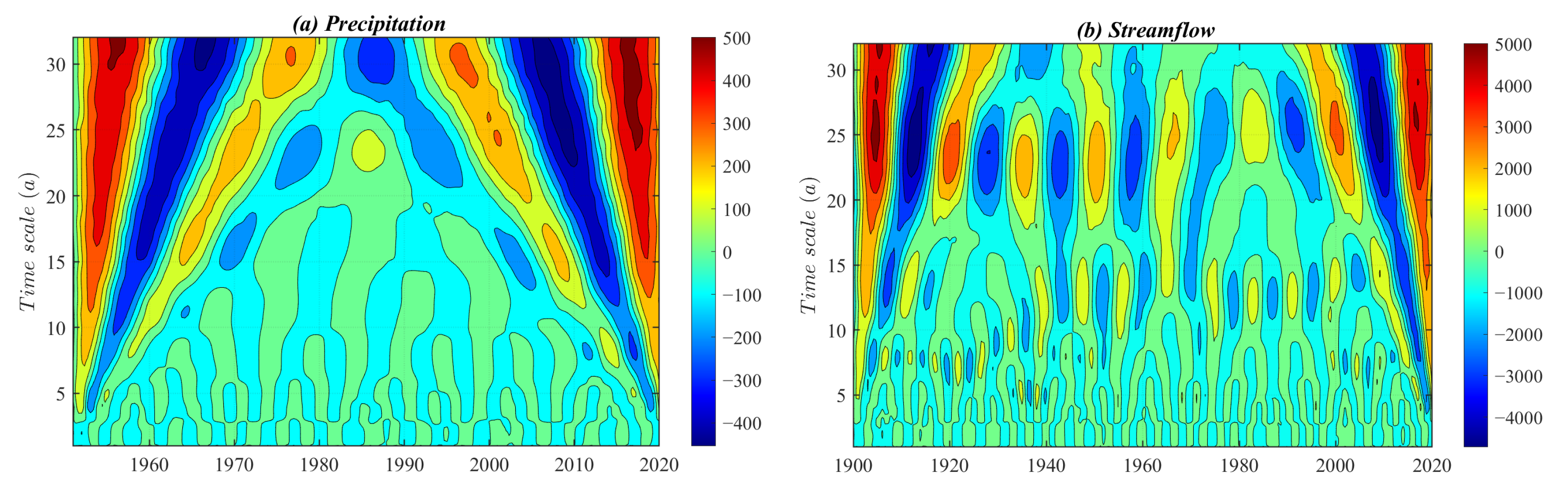
The contour map of the wavelet coefficients’ real part reflects periodic variations of time series at different scales and their distribution in the time domain so as to judge the future trends of precipitation and streamflow at different timescales. Wavelet coefficient contour maps of annual precipitation and annual streamflow series are given by Figure 4, which depict multi-timescale characteristics that exist in the evolutionary process of precipitation and streamflow. Horizontal coordinates denote years; vertical coordinates denote timescale (a); and equivalence curves denote real part values of wavelet coefficients, where positive values denote abundant water periods and negative values denote withered water periods.

Figure 4 shows that four scale types of periodic variation patterns exist in precipitation evolutionary process including 26–32-, 20–25-, 12–18- and 4–10-year. Quasi-3.5 oscillations of alternating abundance–withering occur on a 26–32-year interdecadal scale; quasi-4.5 oscillations occur on a 20–25-year interdecadal scale, and periodic variation of both interdecadal scales exhibits highly stability over the whole study time domain. Moreover, periodic variations on a 12–18-year interdecadal scale show quasi-4 oscillations during the periods of 1950 to 1975 and 2000 to 2020; a 4–10-year interannual scale shows relatively stable performance during the 1950s and 2010s. Four scale types of periodic variation patterns exist in streamflow evolutionary process, including 26–32-, 20–25-, 12–18- and 4–10-year. Quasi-7.5 oscillations of alternating abundance–withering occur on an 18–32-year interdecadal scale; quasi-11 oscillations occur on a 10–17-year interdecadal scale. Moreover, periodic variation on an 18–32-year interdecadal scale shows stability and continuity throughout the time domain; periodic variation on a 10–17-year interdecadal scale shows relatively stability after the 1940s; and a 4–9-year interannual scale shows relative stability during the periods of 1900 to 1940 and 2000 to 2020.

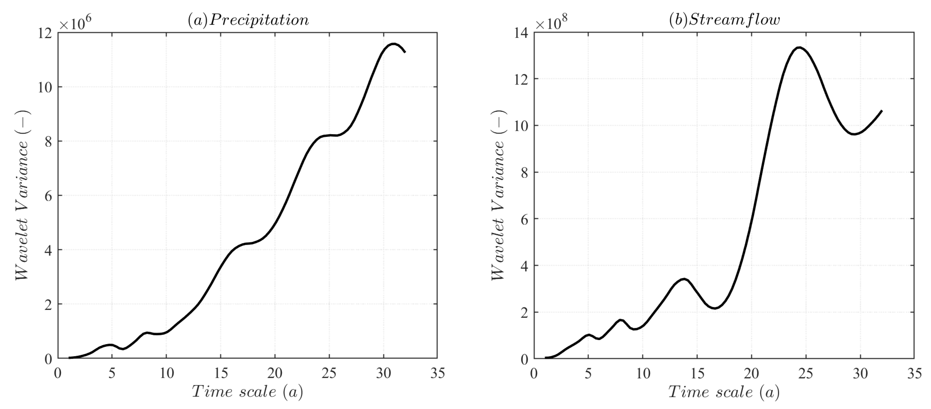
Wavelet variance maps are given by Figure 5, which are used to determine the main cycle present in evolutionary process of precipitation and streamflow. Horizontal coordinates denote timescale (a); vertical coordinates denote wavelet variance, reflecting the energetic distribution of time series fluctuating with scale (a). Five significant crest values exist in wavelet variance maps of precipitation, corresponding to 31-, 24-, 17-, 8- and 5-year timescales, respectively. The maximum peak corresponds to a 31-year timescale, indicating the strongest cyclic oscillation around 31 years, which is first main cycle of precipitation variation; 24-year timescale corresponds to the second peak, which is second main cycle of precipitation variation; the third, fourth and fifth peaks correspond to 17-, 8- and 5-year timescales, respectively, in the order of third, fourth and fifth main cycles of precipitation. Fluctuations in these five cycles control the changing characteristics of precipitation over the whole study time domain (from 1951 to 2020). Four distinct peaks exist in wavelet variance maps of streamflow, corresponding to 24-, 14-, 8- and 5-year timescales in turn. The maximum peak corresponds to a 24-year timescale, indicating the strongest cyclic oscillation around 24 years, the first main cycle of annual streamflow variation; the second peak corresponds to a 14-year timescale, the second main cycle of streamflow variation; the third and fourth peaks correspond to 8- and 5-year timescales, i.e., the third and fourth main cycles of streamflow in the UYRB, respectively. Fluctuations in these four timescales control evolutionary characteristics of streamflow throughout the whole study time domain (from 1900 to 2020).

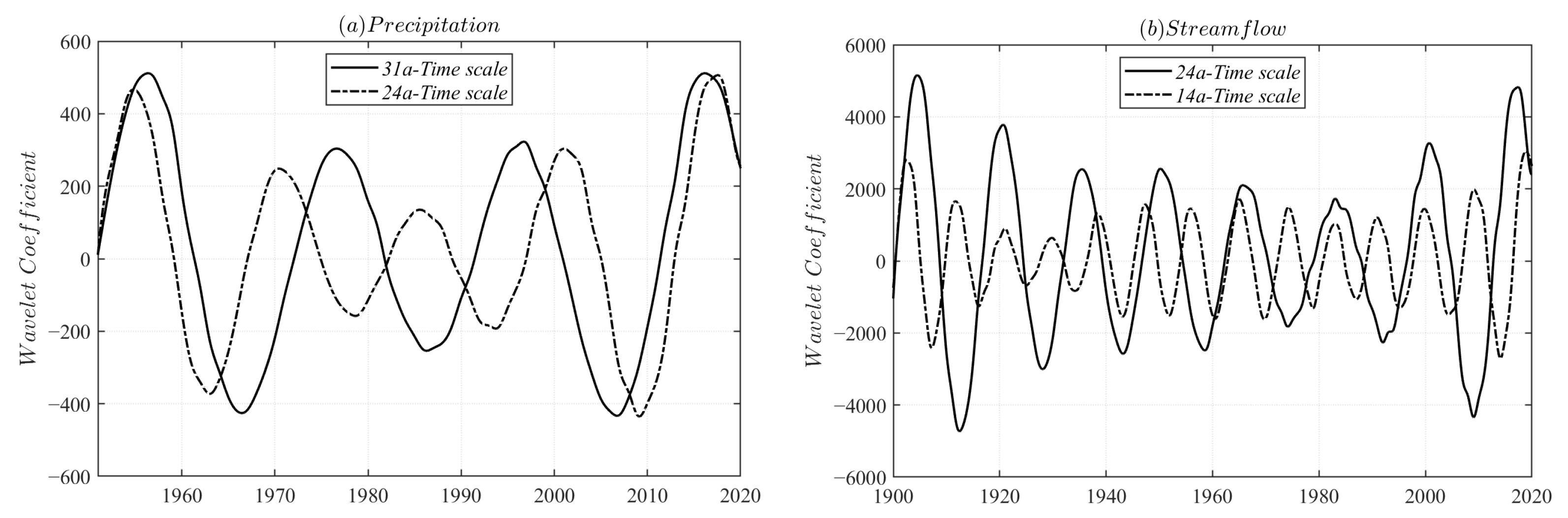
Wavelet coefficient maps of the first and second main cycles controlling the evolution of precipitation and streamflow were plotted based on the wavelet variance test results. The principal period trend maps reflect the average period and abundant-withering variation characteristics of precipitation and streamflow series existing at different timescales. Figure 6 shows that on a 31-year characteristic timescale, the average cycle of precipitation variation is about 21 years, which undergoes about 3.5 periods of abundance–depletion transitions during the study period; on a 24-year characteristic timescale, the average cycle is about 16 years, undergoing about 4.5 cycles of abundance–depletion variation. On a 24-year characteristic timescale, the average cycle of streamflow variation is about 16 years, which undergoes about 7.5 periods of abundance–depletion transitions during the study period; on a 14-year characteristic timescale, the average cycle is about 9 years, undergoing about 13.5 cycles of abundance–depletion variation.

4.2. XWT between Hydrological Variables and Teleconnections

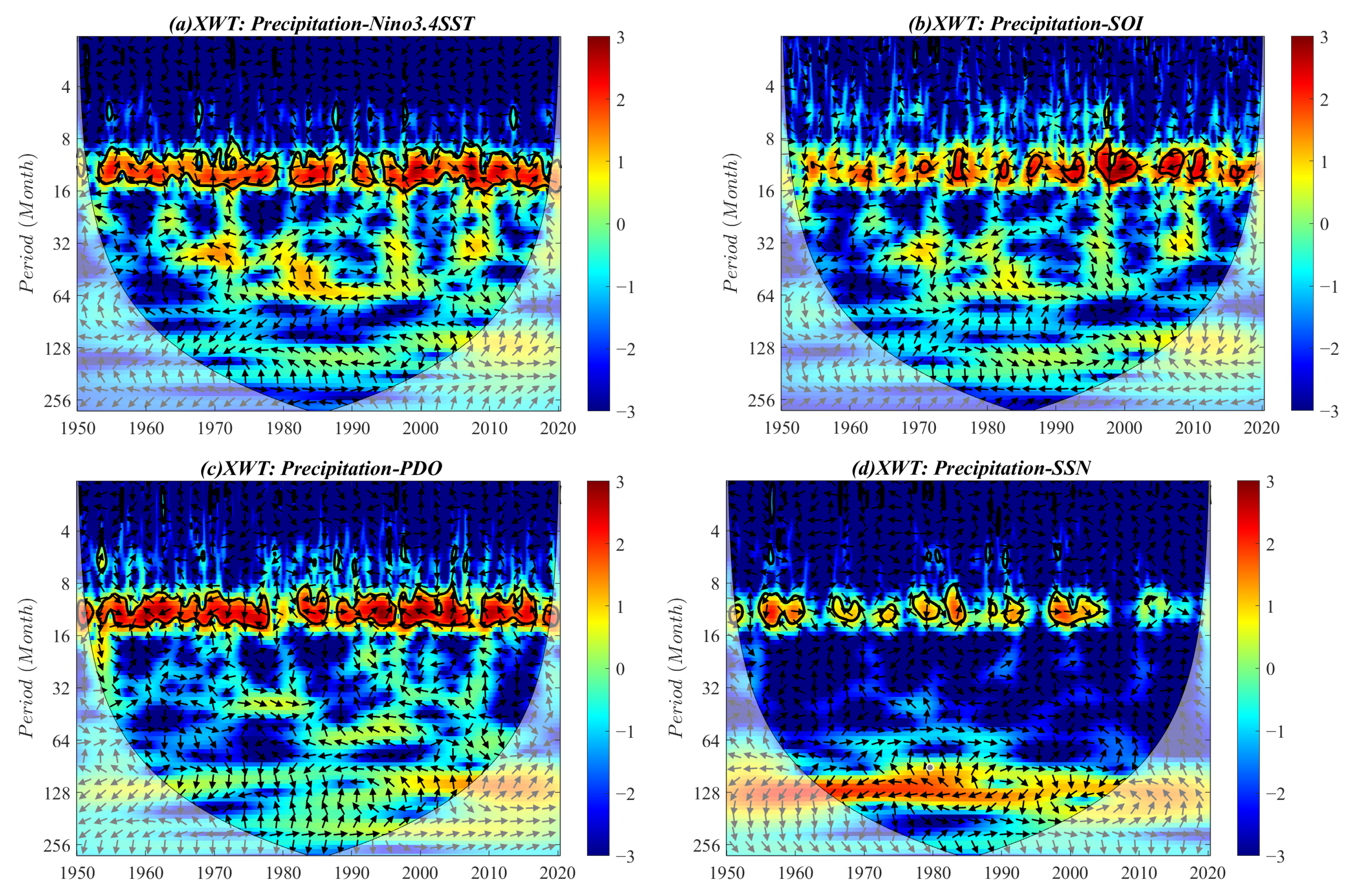
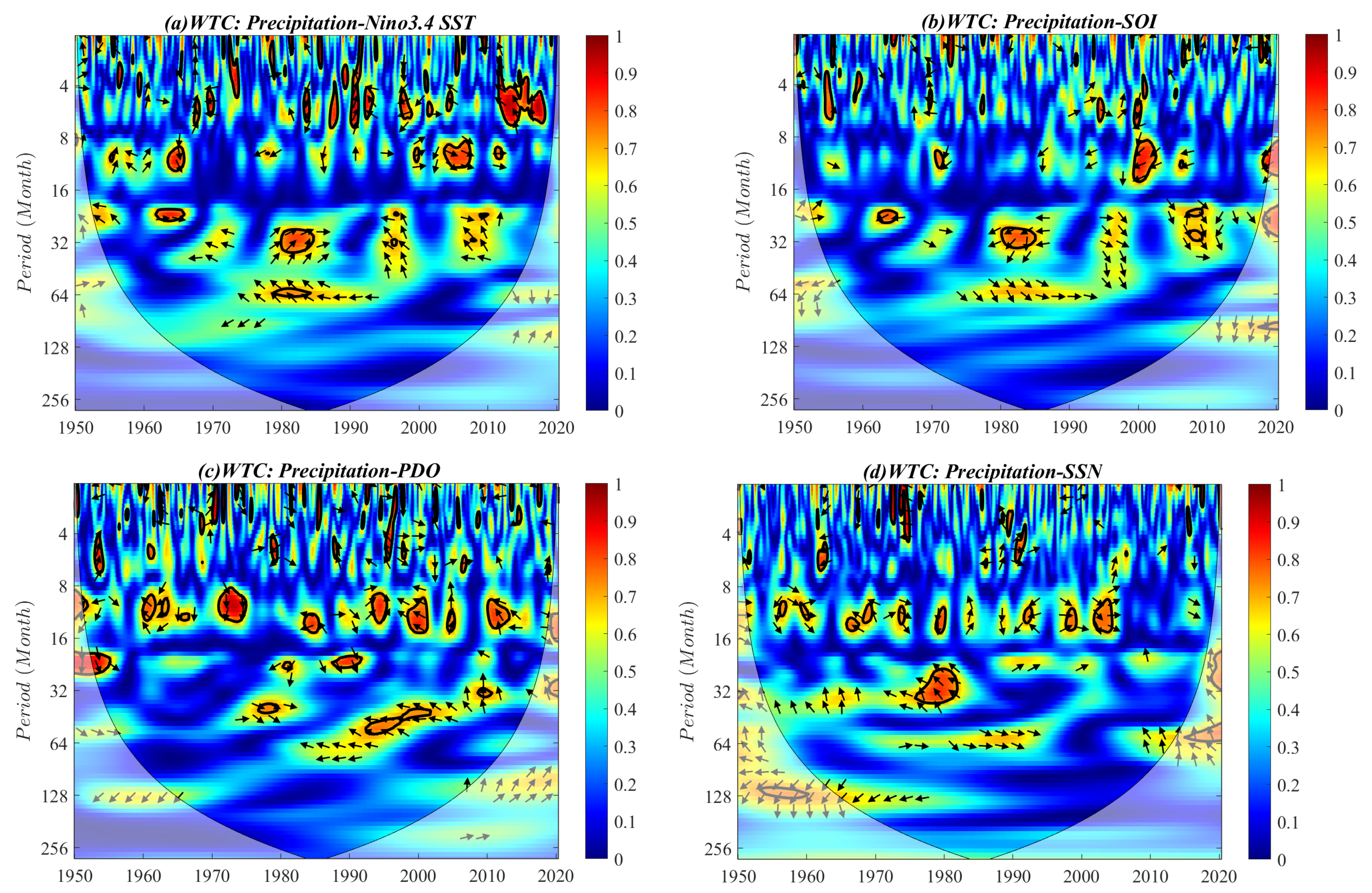
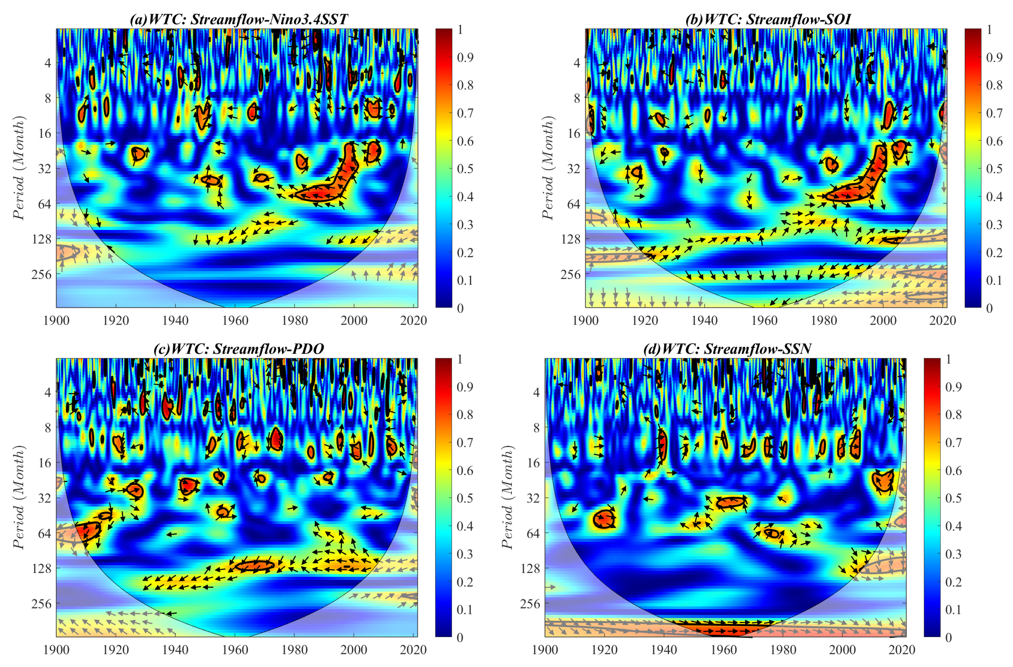
Time-frequency multiscale correlations at different phases were investigated with the purpose of characterizing the dependency of hydrological factors on ocean–atmosphere phenomena and sunspot activity. The thin black soild line in the cross-wavelet spectrum and wavelet coherence spectrum denotes the cone of influence (COI) with boundary effect; the thick black contour denotes passing the red noise inspection with 95% confidence level, i.e., significant correlation. The arrows towards the right denote that hydrological variables and telecorrelations vary in-phase, i.e., positive correlation; the arrows toward the left denote anti-phase variation, i.e., negative correlation; the downward arrows denote that hydrological variables vary 90° ahead of telecorrelations, i.e., 3 months; the updward arrows denote lagging the variation of telecorrelations by 90°.

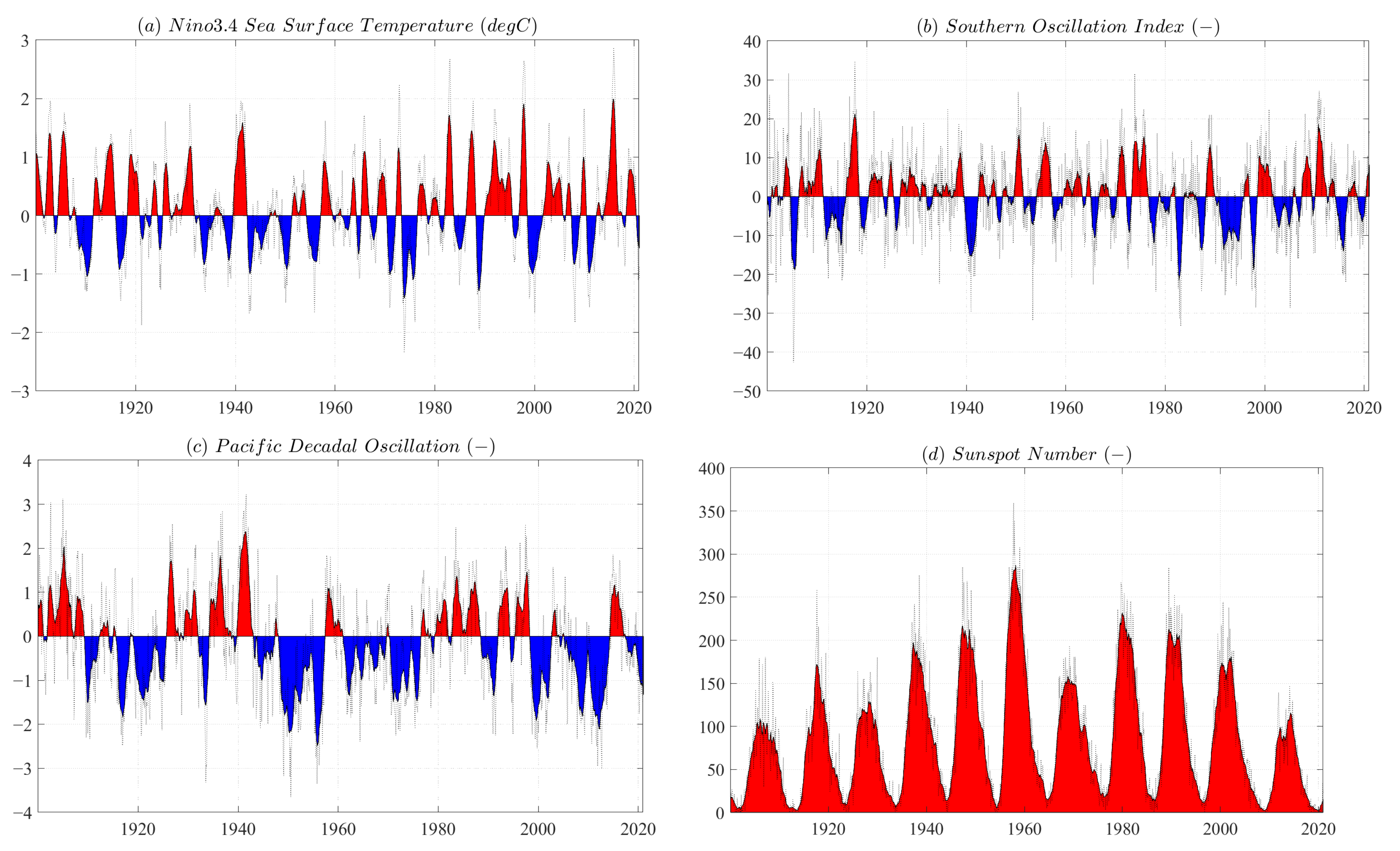
Figure 7 depicts cross-wavelet transform results between monthly precipitation series in the UYRB and contemporaneous monthly scale telecorrelational indexes, among which Nino3.4 SST and SOI characterize ENSO; PDO characterizes PDO; and SSN characterizes sunspot activity. Precipitation and Nino3.4 region SSTs exhibit highly significant 8–16-month main resonance cycle throughout the study time domain, yet the phase relation varies considerably with time domain variations. Furthermore, an intermittent antiphase resonance cycle of about 28–64-months occured during 1965 to 2010, with a lag of about 4.5 months in precipitation variation (mean phase angle about 135°), yet it was insignificant at 95% confidence level. Precipitation and SOI exhibit a significant intermittent 8–14-month resonance cycle within time domain, with phase variation over time and instability in correlation. The continuous and significant 8–14-month resonance cycle between precipitation and PDO exists throughout the study time domain, manifesting mainly as antiphase variation, and a lag relative to PDO exists in precipitation during 1982 to 2018. Precipitation and SSN exhibit intermittent 10–14-month resonance cycles during 1955 to 2005 while passing the significance test. Precipitation shows a relatively strong antiphase resonance cycle, with SSN on an interdecadal scale of approximately 128 months, yet insignificant at 95% confidence level. Additionally, the cross-wavelet energy intensity discontinuously passing the significance test exists for precipitation and telecorrelation indexes in the 1–6-month frequency band; however, durations are short and phase relationships vary widely with time, and the correlation is unstable.

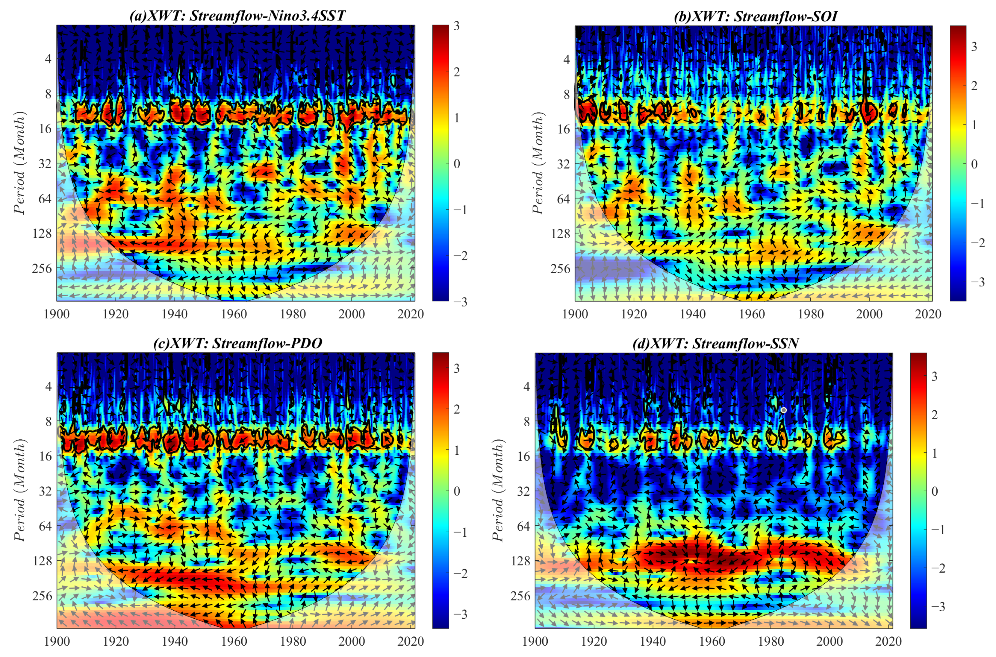
Figure 8 depicts cross-wavelet transform results between monthly streamflow series in the UYRB and contemporaneous monthly telecorrelation indexes. Streamflow series exhibited an intermittent and highly significant 8–16-month main resonance cycle with Nino3.4 SST, with in-phase variation and a lag of about 1.5 months in streamflow during 1905 to 1925 and 1995 to 2015 (mean phase angle of about 45°). Moreover, streamflow and Nino3.4 SST exhibit intermittent relatively strong resonance cycles on the interannual scales of 28–64- and 64–128-month, yet insignificant at 95% confidence level; a continuous strong resonance cycle exists on the interdecadal scale of 128–224-month, with the two showing antiphase variation during 1920 to 1960 and 1990 to 2010; the period of 1960 to 1990 manifested in-phase variation, with a failure to pass red noise tests of 95% confidence level. Streamflow and SOI exhibited a significant resonance cycle of intermittent 8–16-month during 1900 to 1940 and 1960 to 2010. Intermittent relatively strong resonance cycles existed on 32–64- and 64–128-month interannual scales and an 128–224-month interdecadal scale, yet they were insignificant at 95% confidence level. Streamflow and PDO exhibit an extremely significant 8–14-month resonance cycle throughout the study time domain. The interannual scale resonance cycles of 48–72 and 72–128 months are located in the period of 1930 to 1960 and 1960 to 2010, respectively, with the two varying in antiphase, yet insignificant at 95% confidence level. Furthermore, strong resonance cycles of 128–256- and 192–256-month interdecadal scales lie on the period of 1920 to 1960 and 1960 to 2020, respectively, while positive and negative correlations alternate before and after 1960, with antiphase before 1960, i.e., negative correlation, and in-phase after 1960 with a lagging effect in streamflow variation. A significant resonance cycle of intermittent 8–14-month timescale existed during 1920 to 2005 between streamflow and SSN, yet the phase dependence varies widely with time domain and correlation is unstable. A continuous stronger resonance cycle of 95–192-month interdecadal scale is located in the period of 1915–2008, while the two showed in-phase, antiphase and in-phase variation during the periods of 1935–1955, 1955–1980 and 1980–2008, respectively, yet they failured to pass red noise tests of 95% confidence level.

4.3. WTC between Hydrological Variables and Teleconnections

WTC measures the coherence of cross-wavelet transform in time-frequency domains [64], which is a correlation coefficient localized in time and frequency space used to quantify the degree of linear relations between hydrological variables and teleconnection index series in the time and frequency domains [66].

Figure 9 depicts wavelet coherence calculation results between monthly precipitation in the UYRB and contemporaneous monthly scale telecorrelation index series. Wavelet energy intensity between precipitation and Nino3.4 SST intermittently pass the significance test on the 1–12-month intra-annual scale and 20–64-month interannual scale, respectively. A significant resonance cycle of 4–7-month scale with a lag in precipitation of about 4 months (mean phase angle of 120°) exists during 2010 to 2018; a significant resonance cycle of 28–38-month scale with in-phase variation and a lag in precipitation of about 1 month (mean phase angle of 30°) exists during 1980 to 1985. Precipitation and SOI exhibit intermittent significant cycles on 1–16- and 20–64-month timescales. Significant antiphase resonance cycles existed on 28–36- and 8–15-month scales within the 1980 to 1986 and 2000 to 2004 periods, respectively; in-phase resonance cycles existed on 56–68-, 20–64-, and 20–48-month interannual scales during 1974 to 1994, 1994 to 1999 and 2004 to 2014 periods, respectively, which failed to pass the red noise tests at 95% significance level. Precipitation and PDO exhibit intermittent significant cycles on 1–14- and 20–64-month scales, with significant periodic correlations on the 8–14-month scale intermittently spanning the time domain, yet phase relationships are less stable. During the period of 1992–2002, a significant interannual resonance cycle of 36–56-month existed with the two showing antiphase variation and a lag of about 5 months in precipitation (mean phase angle of 150°). Intermittent and significant resonance cycles exist between precipitation and SSN on 1–7- and 10–14-month scales during 1962 to 1994 and 1955 to 2005, respectively, while phase relationship remains unstable. Moreover, the significant interannual resonance cycle of 24–36-month emerges during 1976 to 1984, with antiphase variation and a lag of about 4.5 months in precipitation to SSN (mean phase angle of 135°).

Figure 10 depicts wavelet coherence calculation results between monthly streamflow in the UYRB and contemporaneous monthly scale telecorrelation index series. Streamflow and Nino3.4 SST show intermittent significant resonance cycles on both a 1–12-month intra-annual scale and 20–64-month interannual scale, yet with a short duration and phase variation over time, the correlation is unstable. Furthermore, a significant interannual scale resonance cycle of 16–64-month exists during 1980 to 2010, with antiphase variation and a lag of about 4.5 months in streamflow response to Nino3.4 SST (mean phase angle of 135°). Wavelet energy intensity between streamflow and SOI series intermittently the pass significance test on interannual scales of 1–16- and 16–64-month, while the significance interval on the 1–16-month scale is short in duration with unstable phase relationship. During the period of 1980 to 2010, significant 16–64-month interannual scale resonance cycles exist, and the two exhibit identical phase relations, i.e., positive correlation with correlation coefficients of 0.80 to 0.85. Streamflow and PDO exhibit intermittent significant resonance cycles on both the 1–16-month scale and 18–72-month interannual scale, yet with short duration and less stable phase relationships, with the significant resonance cycle on the 48–72-month interannual scale occurring during the period of 1910 to 1920. Moreover, the interdecadal scale correlation of about 128 months occurs continuously within the period of 1930 to 2010 and passes 95% significance test level against red noise during the period of 1960 to 1975 and 1995 to 2002, with correlation coefficients reaching about 0.80. Intermittent significant resonance cycles occur between streamflow and SSN on both the 1–16-month scale and 20–72-month interannual scale. Significant and intermittent correlation on the 8–16-month scale occur during 1940 to 2010, dominated by co-phase variations. Significant resonance cycle on an interannual scale of 16–28-month occurs during the period of 2010 to 2018, with a lag of about 3 months in streamflow response to SSN (mean phase angle of 90°). A 32–64-month interannual scale exhibits significant resonance cycles during the periods of 1915–1925, 1955–1970 and 1972–1980. Moreover, streamflow and SSN manifest a continuous and highly significant interannual main resonance cycle of 320–448 months throughout the time domain, with the two showing in-phase variation, i.e., positive correlation.

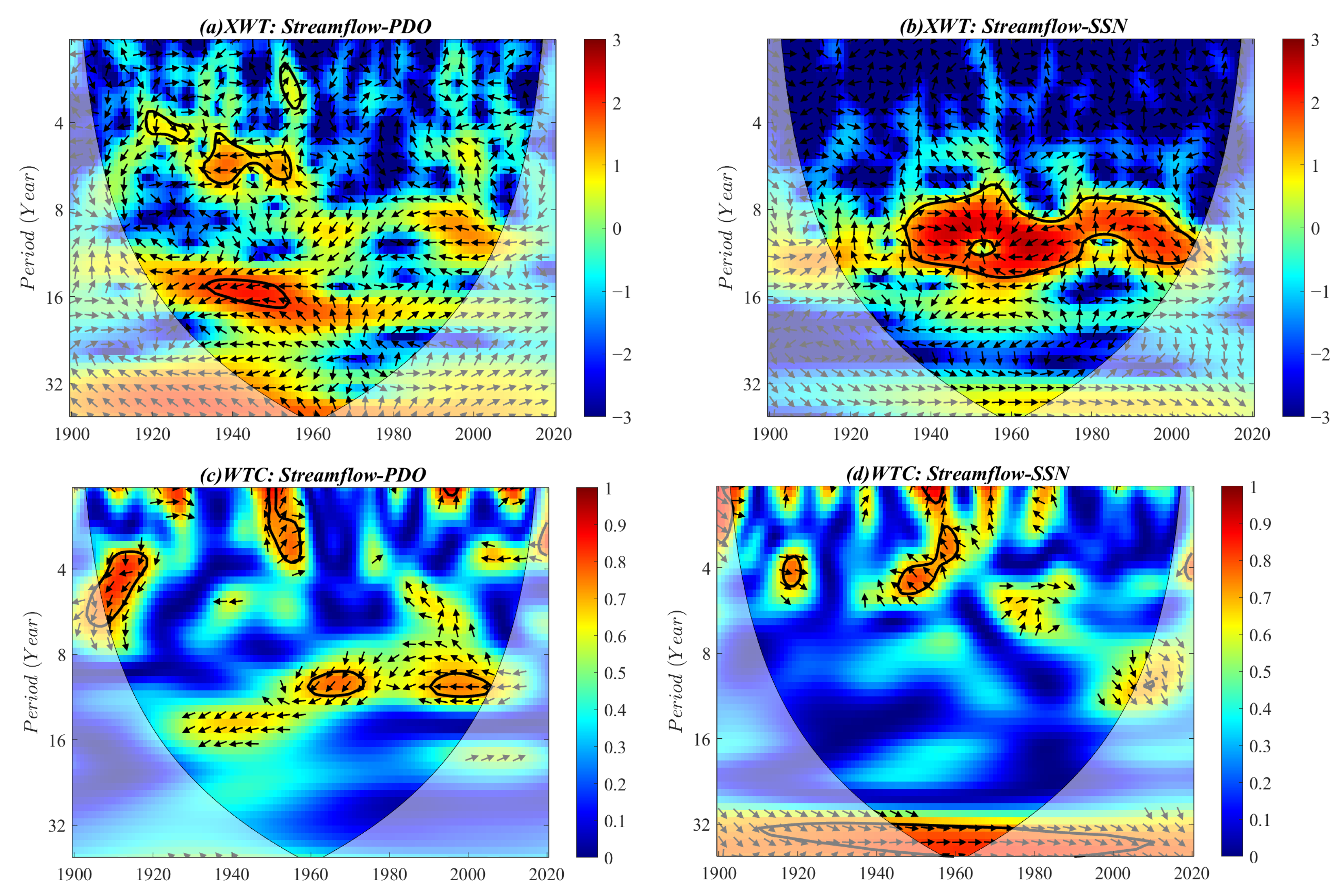
4.4. XWT and WTC between Annual Streamflow and PDO/SSN

According to the aforementioned results, streamflow in the UYRB are significantly correlated with PDO and SSN on interdecadal scales; thus, further cross-wavelet transform and wavelet coherence were performed between annual streamflow from 1900 to 2020 and contemporaneous annual PDO and SSN time series to analyze the possible influence of interdecadal scale periodic oscillations of PDO and sunspot activity on streamflow evolution in the UYRB. The calculation results are given in Figure 11.

Figure 11 indicates that streamflow and PDO exhibit significant negative correlations on a 4–7-year interannual scale and 14–18-year interdecadal scale resonance cycles at 95% confidence level, with the interdecadal scale resonance cycle being predominant. Streamflow and SSN exhibit a longer interannual and interdecadal main resonance cycle on the 7–14-year scale and pass the red noise test at 95% significant level during the period of 1934 to 2008. The two show positive, negative and positive correlations during the 1934–1955, 1955–1980 and 1980–2008 periods, respectively. Resonance cycle on the 8–16-year scale with inverse phase between streamflow and PDO occurs during 1928 to 2008, and negative correlations on the 10–12-year interdecadal scale pass 95% confidence level of the red noise test during 1960 to 1975 and 1990 to 2005. Moreover, 3–7- and 1–4-year interannual resonance cycles were observed during the periods of 1906–1920 and 1950–1960, respectively. Streamflow and SSN exhibit a significant 32–48-year interdecadal scale main resonance cycle with positive correlation at 95% confidence level. Moreover, a significant 1–6-year interannual scale resonance cycle appears during the period of 1945 to 1962, with a lagged response approximately 4 years in streamflow to SSN (mean phase angle of 120°).

5. Discussion

ENSO manifests as wind field and sea surface temperature oscillations in equatorial east-central Pacific, originating from ocean–atmosphere interactions at low latitudes. Nino3.4 SST and SOI were used to characterize ENSO signals, and the results indicate that multiple significant interannual resonance cycles exist between hydrometeorological factors in the UYRB and ENSO signals, yet the phase relationships vary with both time and frequency domains. ENSO shows significant correlation with precipitation mainly on the 4–12-month intra-annual scale and 12–64-month interannual scale, with streamflow mainly on 12–64-month interannual scale; hence, anomalous interannual fluctuations of ENSO events exert important implications for shorter interannual scale cycle variations of both precipitation and streamflow in the UYRB.

PDO represents a strong periodic pattern of ocean–atmospheric variability centered on the mid-latitude Pacific basin. The PDO index was used to characterize PDO signals, and the results indicate that PDO primarily affects periodic variation on a longer interannual scale of precipitation and about 10-year interdecadal scale of streamflow in the UYRB. PDO exhibits a significant negative correlation with precipitation on a 48–64-month interannual scale, yet the covariance varies over time-domain, while there is a steady and continuous negative correlation with streamflow on about 10-year interdecadal scale. Previous research has shown that among numerous oceanic–atmospheric signals, PDO was the ocean signal that best explained variations in the Yangtze streamflow [66]. Positive PDO corresponds to a low precipitation period, further affecting long-term water discharge of the Yangtze River [69]. Moreover, water discharge from the Yangtze River consists of cycles that are close to the typical PDO cycles (i.e., 15- to 20-year cycles, on average) [52,66], which is consistent with the conclusion of the present research.

Furthermore, interdecadal scale periodic oscillations of PDO have stronger and more consistently significant effects on streamflow than precipitation in the UYRB. This conclusion could be supported by the view that on account of the variability in precipitation that is more enhanced than in streamflow, and that streamflow integrates information spatially, the relationship between streamflow and telecorrelation might be stronger than that between precipitation and telecorrelation [11,70]. According to Beebee and Manga [17], this may be due to the spatial advantage of streamflow that stream discharge represents a more coherent spatial average over a smaller area than scattered climate stations, or because runoff depends on both precipitation and temperature associated with evapotranspiration, and hydrologic cycle amplifies the combined effects of precipitation and temperature, or both included.

The 11-year quasi-periodic oscillations in sunspot activity affect climatic variations on global scales. Sunspot number (SSN) was adopted to characterize sunspot activity, and the results indicate that sunspot activity has significant effects on the interdecadal scale cyclic variation of streamflow more than precipitation variation, which mainly manifests in that SSN exhibits significant negative yet unstable correlation with precipitation mainly on a 24–36-month interannual scale, while it has extremely stable and consistently significant positive correlation with streamflow on a 32–48-year interdecadal scale. Additionally, the main resonance cycles of SSN and both annual precipitation and streamflow are located on an 8–14-year timescale, suggesting that the 11-year cycle fluctuations of sunspots have important effects on the interdecadal scale periodic variability of precipitation and streamflow in the UYRB. Consequently, investigations on the possible effects of interannual scale variability of ENSO and interdecadal scale variability of PDO and sunspot activity on hydrometeorological factors in the UYRB should be strengthened in the future.

Under changing climate scenarios and changing atmospheric and oceanic conditions, an effective and promising approach to forecast hydrological factors is to focus on the best predictors [66]. The results contribute to better understanding of long-term trends in precipitation and streamflow over the UYRB and their multi-scale correlations with Pacific oceanic–atmospheric singals and astronomical factor, further providing meaningful information for planning and implementing operational strategies for sustainable utilization of local water resources.

6. Conclusions

The possible effects of different time-scale periodic oscillations in both oceanic atmospheric signals and solar activity on the evolution of precipitation and streamflow in specific watersheds provide useful information for scientifically forecasting local water resources and water-related management. The present research estimated the main variability timescales of the precipitation and streamflow in the Upper Yangtze River Basin (UYRB) and their relations to the large-scale climate variablity, with the research results summarized as follows.

(1) Continuous wavelet transform results indicate that both precipitation and streamflow series exhibit significant interannual oscillations during the whole study period, with continuous annual periodicity spanning the entire time domain. The first and second principal periods of annual precipitation variation correspond to 31- and 24-year timescales, respectively, and the first and second principal periods of annual streamflow correspond to 24- and 14-year timescales, respectively. In addition, significant periodic oscillations exist in both precipitation and streamflow on 8- and 5-year time scales.

(2) Cross-wavelet and wavelet coherence spectrums indicate that significant correlation between precipitation and ENSO are mainly located on an interannual scale of 1–4 years; significant correlation with PDO are located on an interannual scale of 1–5 years and the two exhibit stable antiphase variation, i.e., negative correlation, on an interannual scale of 3–5 years; an intermittent significant correlation with SSN lies on an interannual scale of 1–3 years, while an interdecadal correlation lies at approximately 11 years, insignificant at 95% confidence level.

(3) Cross-wavelet and wavelet coherence spectrums indicate that a significant correlation between streamflow and ENSO is located on interannual scale of 1–5 years, with insignificance on an interdecadal scale of approximately 10 years; intermittent significant correlation with PDO on an interannual scale of 1–6 years, while a stable negative correlation is located on an interdecadal scale of 10–16 years, passing the 95% significance test; intermittent significant correlation with SSN on an interannual scale of 1–6 years, with a consistent and continuous significant positive correlation located on a relatively long interdecadal scale of 32–48 years.

(4) Overall, ENSO mainly affects short interannual periodic fluctuations of precipitation and streamflow in the UYRB, with phase relationships varying widely over time; PDO and SSN mainly affect interannual periodic variability of precipitation and interannual and interdecadal periodic variability of streamflow, where the interdecadal scale is affected more steadily and consistently than the interannual scale. Analysis indicates that PDO and SSN have stronger influences on streamflow variability than precipitation in the UYRB, and interdecadal scale correlations of both PDO and SSN to streamflow continuously act on interdecadal periodic variability of streamflow.

References

1. Wei, X.; Cai, S.; Ni, P.; Zhan, W. Impacts of climate change and human activities on the water discharge and sediment load of the Pearl River, southern China. Sci. Rep. 2020, 10, 16743. [Google Scholar] [CrossRef]
2. Yoon, J.H.; Wang, S.Y.; Gillies, R.; Kravitz, B.; Hipps, L.; Rasch, P. Increasing water cycle extremes in California and in relation to ENSO cycle under global warming. Nat. Commun. 2015, 6, 8657. [Google Scholar] [CrossRef] [Green Version]
3. Canchala, T.; Cerón, W.L.; Francés, F.; Carvajal-Escobar, Y.; Andreoli, R.; Kayano, M.; Alfonso-Morales, W.; Caicedo-Bravo, E.; Souza, R. Streamflow Variability in Colombian Pacific Basins and Their Teleconnections with Climate Indices. Water 2020, 12, 526. [Google Scholar] [CrossRef] [Green Version]
4. Coulibaly, P. Spatial and temporal variability of Canadian seasonal precipitation (1900–2000). Adv. Water Resour. 2006, 29, 1846–1865. [Google Scholar] [CrossRef]
5. Ahmed, N.; Wang, G.; Booij, M.; Oluwafemi, A.; Hashmi, M.; Ali, S.; Munir, S. Climatic Variability and Periodicity for Upstream Sub-Basins of the Yangtze River, China. Water 2020, 12, 842. [Google Scholar] [CrossRef] [Green Version]
6. Jiang, R.; Gan, T.; Xie, J.; Wang, N. Spatiotemporal variability of Alberta’s seasonal precipitation, their teleconnection with large-scale climate anomalies and sea surface temperature. Int. J. Climatol. 2013, 34, 2899–2917. [Google Scholar] [CrossRef]
7. Pasquini, A.; Depetris, P. Discharge trends and flow dynamics of South American rivers draining the southern Atlantic seaboard: An overview. J. Hydrol. 2007, 333, 385–399. [Google Scholar] [CrossRef]
8. Wanders, N.; Wada, Y. Decadal predictability of river discharge with climate oscillations over the 20th and early 21st century. Geophys. Res. Lett. 2015, 42, 10689–10695. [Google Scholar] [CrossRef] [Green Version]
9. Zhang, H.; Cheng, H.; Spötl, C.; Cai, Y.; Sinha, A.; Tan, L.; Yi, L.; Yan, H.; Kathayat, G.; Ning, Y.; et al. A 200-year annually laminated stalagmite record of precipitation seasonality in southeastern China and its linkages to ENSO and PDO. Sci. Rep. 2018, 8, 12344. [Google Scholar] [CrossRef] [Green Version]
10. Dettinger, M.; Cayan, D.; McCabe, G.; Marengo, J. Multiscale streamflow variability associated with el niño/southern oscillation. In El Niño and the Southern Oscillation–Multiscale Variability and Global and Regional Impacts; Diaz, H., Markgraf, V., Eds.; Cambridge University Press: Cambridge, UK, 2000; pp. 113–146. ISBN 978-0-521-62138-0. [Google Scholar]
11. Emerton, R.; Cloke, H.; Stephens, E.; Zsoter, E.; Woolnough, S.; Pappenberger, F. Complex picture for likelihood of ENSO-driven flood hazard. Nat. Commun. 2017, 8, 14796. [Google Scholar] [CrossRef] [Green Version]
12. Hu, Z.; Kumar, A.; Zhu, J.; Huang, B.; Tseng, Y.; Wang, X. On the Shortening of the Lead Time of Ocean Warm Water Volume to ENSO SST Since 2000. Sci. Rep. 2017, 7, 4294. [Google Scholar] [CrossRef] [PubMed] [Green Version]
13. Torrence, C.; Webster, P. Interdecadal changes in the ENSO–monsoon system. J. Clim. 1999, 12, 2679–2690. [Google Scholar] [CrossRef] [Green Version]
14. Glantz, M.; Katz, R.; Nicholls, N. Teleconnections Linking Worldwide Climate Anomalies: Scientific Basis and Societal Impact; Glantz, M., Katz, R., Nicholls, N., Eds.; Cambridge University Press: Cambridge, UK, 1991; ISBN 978-0-521-36475-1. [Google Scholar]
15. Mantua, N.; Hare, S.; Zhang, Y.; Wallace, J.; Francis, R. A Pacific Interdecadal Climate Oscillation with Impacts on Salmon Production. Bull. Am. Meteorol. Soc. 1997, 78, 1069–1080. [Google Scholar] [CrossRef]
16. McCabe, G.; Dettinger, M. Primary Modes and Predictability of Year-to-Year Snowpack Variations in the Western United States from Teleconnections with Pacific Ocean Climate. J. Hydrometeorol. 2002, 3, 13–25. [Google Scholar] [CrossRef]
17. Beebee, R.; Manga, M. Variation in the Relationship Between Snowmelt Runoff In Oregon and ENSO And PDO. J. Am. Water Resour. Assoc. 2004, 40, 1011–1024. [Google Scholar] [CrossRef]
18. Harshburger, B.; Ye, H.; Dzialoski, J. Observational evidence of the influence of Pacific SSTs on winter precipitation and spring stream discharge in Idaho. J. Hydrol. 2002, 264, 157–169. [Google Scholar] [CrossRef]
19. Hanson, R.; Newhouse, M.; Dettinger, M. A methodology to asess relations between climatic variability and variations in hydrologic time series in the southwestern United States. J. Hydrol. 2004, 287, 252–269. [Google Scholar] [CrossRef]
20. Jain, S.; Lall, U. Floods in a changing climate: Does the past represent the future? Water Resour. Res. 2001, 37, 3193–3205. [Google Scholar] [CrossRef]
21. Hidalgo, H.; Dracup, J. ENSO and PDO Effects on Hydroclimatic Variations of the Upper Colorado River Basin. J. Hydrometeorol. 2003, 4, 5–23. [Google Scholar] [CrossRef]
22. Wang, G.; Zhao, C.; Zhang, M.; Zhang, Y.; Lin, M.; Qiao, F. The causality from solar irradiation to ocean heat content detected via multi-scale Liang–Kleeman information flow. Sci. Rep. 2020, 10, 17141. [Google Scholar] [CrossRef]
23. Wu, Y.; He, Y.; Wu, M.; Chen, L.; Gao, S.; Xu, Y. Multifractality and cross-correlation analysis of streamflow and sediment fluctuation at the apex of the Pearl River Delta. Sci. Rep. 2018, 8, 16553. [Google Scholar] [CrossRef]
24. Camp, C.; Tung, K. Surface warming by the solar cycle as revealed by the composite mean difference projection. Geophys. Res. Lett. 2007, 34, L14703. [Google Scholar] [CrossRef] [Green Version]
25. Zhou, J.; Tung, K. Solar Cycles in 150 Years of Global Sea Surface Temperature Data. J. Clim. 2010, 23, 3234–3248. [Google Scholar] [CrossRef] [Green Version]
26. Meehl, G.; Arblaster, J.; Branstator, G.; Loon, H. A Coupled Air–Sea Response Mechanism to Solar Forcing in the Pacific Region. J. Clim. 2008, 21, 2883–2897. [Google Scholar] [CrossRef] [Green Version]
27. Hanson, E.; Okeke, F. Impacts of sunspot number and Geomagnetic aa-index on climate of Wet Zone West Africa during solar cycles 22–24. Sci. Rep. 2021, 11, 11500. [Google Scholar] [CrossRef] [PubMed]
28. Reid, G. Influence of solar variability on global sea surface temperatures. Nature 1987, 329, 142–143. [Google Scholar] [CrossRef]
29. White, W.; Lean, J.; Cayan, D.; Dettinger, M. Response of global upper ocean temperature to changing solar irradiance. J. Geophys. Res. 1997, 102, 3255–3266. [Google Scholar] [CrossRef]
30. Cerón, W.; Kayano, M.; Andreoli, R.; Avila, A.; Canchala, T.; Francés, F.; Rivera, I.; Alfonso-Morales, W.; Souza, R.; Carvajal-Escobar, Y. Streamflow Intensification Driven by the Atlantic Multidecadal Oscillation (AMO) in the Atrato River Basin, Northwestern Colombia. Water 2020, 12, 216. [Google Scholar] [CrossRef] [Green Version]
31. Coulibaly, P.; Burn, D. Wavelet analysis of variability in annual Canadian streamflows. Water Resour. Res. 2004, 40, W03105. [Google Scholar] [CrossRef]
32. Ha, S.; Liu, D.; Mu, L. Prediction of Yangtze River streamflow based on deep learning neural network with El Niño–Southern Oscillation. Sci. Rep. 2021, 11, 11738. [Google Scholar] [CrossRef]
33. Xiao, M.; Zhang, Q.; Singh, V. Influences of ENSO, NAO, IOD and PDO on seasonal precipitation regimes in the Yangtze River basin, China. Int. J. Climatol. 2015, 35, 3556–3567. [Google Scholar] [CrossRef]
34. Jiang, T.; Su, B.; Hartmann, H. Temporal and spatial trends of precipitation and river flow in the Yangtze River Basin, 1961–2000. Geomorphology 2007, 85, 143–154. [Google Scholar] [CrossRef]
35. Yuan, N.; Fu, Z.; Zhang, H.; Piao, L.; Xoplaki, E.; Luterbacher, J. Detrended Partial-Cross-Correlation Analysis: A New Method for Analyzing Correlations in Complex System. Sci. Rep. 2015, 5, 8143. [Google Scholar] [CrossRef] [Green Version]
36. Xu, K.; Brown, C.; Kwon, H.; Lall, U.; Zhang, J.; Hayashi, S.; Chen, Z. Climate teleconnections to Yangtze river seasonal streamflow at the Three Gorges Dam, China. Int. J. Climatol. 2007, 27, 771–780. [Google Scholar] [CrossRef] [Green Version]
37. Yuan, N.; Xoplaki, E.; Zhu, C.; Luterbacher, J. A novel way to detect correlations on multi-timescales, with temporal evolution and for multi-variables. Sci. Rep. 2016, 6, 27707. [Google Scholar] [CrossRef] [Green Version]
38. Dong, X. Influences of the Pacific Decadal Oscillation on the East Asian Summer Monsoon in non–ENSO years. Atmos. Sci. Lett. 2016, 17, 115–120. [Google Scholar] [CrossRef]
39. Zhang, R.; Xu, Z.; Zuo, D.; Ban, C.H. Hydro-Meteorological Trends in the Yarlung Zangbo River Basin and Possible Associations with Large-Scale Circulation. Water 2020, 12, 144. [Google Scholar] [CrossRef] [Green Version]
40. Liu, Y.; Ding, Q.; Chen, M.; Zhong, L.; Labat, D.; Zhang, M.; Mao, Y.; Li, Y. Analyses of Runoff and Sediment Transport and their Drivers in a Rare Earth Mine Drainage Basin of the Yangtze River, China. Water 2020, 12, 2283. [Google Scholar] [CrossRef]
41. Huang, H.; Zhang, B.; Cui, Y.; Ma, S. Analysis on the Characteristics of Dry and Wet Periods in The Yangtze River Basin. Water 2020, 12, 2960. [Google Scholar] [CrossRef]
42. Guo, R.; Zhu, Y.; Liu, Y. A Comparison Study of Precipitation in the Poyang and the Dongting Lake Basins from 1960–2015. Sci. Rep. 2020, 10, 3381. [Google Scholar] [CrossRef]
43. Dong, Q.; Fang, D.; Zuo, J.; Wang, Y. Hydrological alteration of the upper Yangtze River and its possible links with large-scale climate indices. Nord. Hydrol. 2019, 50, 1120–1137. [Google Scholar] [CrossRef]
44. Zhu, N.; Xu, J.; Li, K.; Luo, Y.; Yang, D.; Zhou, C. Spatiotemporal Change of Plum Rains in the Yangtze River Delta and Its Relation with EASM, ENSO, and PDO During the Period of 1960–2012. Atmosphere 2019, 10, 258. [Google Scholar] [CrossRef] [Green Version]
45. Xu, Y.; Wu, Y.; Xu, G. Variation of reference evapotranspiration and its teleconnection with multiple large-scale climate oscillations in the Yangtze River Delta, China. Int. J. Climatol. 2019, 39, 2630–2645. [Google Scholar] [CrossRef]
46. Tang, J.; Li, Q.; Chen, J. Summertime runoff variations and their connections with Asian summer monsoons in the Yangtze River basin. J. Water Clim. Chang. 2018, 9, 89–100. [Google Scholar] [CrossRef]
47. Liu, X.; Zhang, Y.; Liu, Y.; Zhao, X.; Zhang, J.; Rui, Y. Characteristics of temperature evolution from 1960 to 2015 in the Three Rivers’ Headstream Region, Qinghai, China. Sci. Rep. 2020, 10, 20272. [Google Scholar] [CrossRef]
48. Li, Z.; Kang, L.; Zhou, L.; Zhu, M. Deep Learning Framework with Time Series Analysis Methods for Runoff Prediction. Water 2021, 13, 575. [Google Scholar] [CrossRef]
49. Wernstedt, K.; Hersh, R. Climate forecasts in flood planning: Promise and ambiguity. J. Am. Water Resour. Assoc. 2002, 38, 1703–1713. [Google Scholar] [CrossRef]
50. Nalley, D.; Adamowski, J.; Biswas, A.; Gharabaghi, B.; Hu, W. A multiscale and multivariate analysis of precipitation and streamflow variability in relation to ENSO, NAO and PDO. J. Hydrol. 2019, 574, 288–307. [Google Scholar] [CrossRef]
51. Tamaddun, K.; Kalra, A.; Ahmad, S. Wavelet analyses of western US streamflow with ENSO and PDO. J. Water Clim. Chang. 2017, 8, 26–39. [Google Scholar] [CrossRef] [Green Version]
52. Zhang, Y.; Wallace, J.; Battisti, D. ENSO–like Interdecadal Variability: 1900–93. J. Clim. 1997, 10, 1004–1020. [Google Scholar] [CrossRef]
53. Mantua, N.; Hare, S. The Pacific Decadal Oscillation. J. Ocean. 2002, 58, 35–44. [Google Scholar] [CrossRef]
54. Minobe, S. A 50–70 year climatic oscillation over the North Pacific and North America. Geophys. Res. Lett. 1997, 24, 683–686. [Google Scholar] [CrossRef] [Green Version]
55. Jolliffe, I.; Cadima, J. Principal component analysis: A review and recent developments. Philos. Trans. R. Soc. A 2016, 374, 20150202. [Google Scholar] [CrossRef]
56. Miró, J.; Caselles, V.; Estrela, M. Multiple imputation of rainfall missing data in the Iberian Mediterranean context. Atmos. Res. 2017, 197, 313–330. [Google Scholar] [CrossRef]
57. Rousi, E.; Anagnostopoulou, C.; Tolika, K.; Maheras, P. Representing teleconnection patterns over Europe: A comparison of SOM and PCA methods. Atmos. Res. 2015, 152, 123–137. [Google Scholar] [CrossRef]
58. Tošić, L.; Zorn, M.; Ortar, J.; Unkašević, M.; Gavrilov, M.; Marković, S. Annual and seasonal variability of precipitation and temperatures in Slovenia from 1961 to 2011. Atmos. Res. 2016, 168, 220–233. [Google Scholar] [CrossRef]
59. Wilks, D. Chapter 12—Principal component (EOF) analysis. In Statistical Methods in the Atmospheric Sciences; Wilks, D., Ed.; Academic Press: New York, NY, USA, 2011; pp. 519–562. ISBN 978-0-12-385022-5. [Google Scholar] [CrossRef]
60. Capozzoli, C.; Cardoso, A.; Ferraz, S. River Flow Variability Patterns in Main Brazilian Basins and Association with Climate Indices. Rev. Bras. Anestesiol. 2017, 32, 243–254. [Google Scholar] [CrossRef] [Green Version]
61. Helena, B.; Pardo, R.; Vega, M.; Barrado, E.; Fernandez, J.; Fernandez, L. Temporal evolution of groundwater composition in an alluvial aquifer (Pisuerga River, Spain) by principal component analysis. Water Res. 2000, 34, 807–816. [Google Scholar] [CrossRef]
62. Sang, Y. A review on the applications of wavelet transform in hydrology time series analysis. Atmos. Res. 2013, 122, 8–15. [Google Scholar] [CrossRef]
63. Holschneider, M. Wavelets: An analysis tool. In Oxford Mathematical Monographs; Oxford University Press: Oxford, UK, 1995; ISBN 978-0-198-50521-1. [Google Scholar]
64. Grinsted, A.; Moore, J.; Jevrejeva, S. Application of the cross wavelet transform and wavelet coherence to geophysical time series. Nonlinear Process. Geophys. 2004, 11, 561–566. [Google Scholar] [CrossRef]
65. Torrence, C.; Compo, G. A Practical Guide to Wavelet Analysis. Bull. Am. Meteorol. Soc. 1998, 79, 61–78. [Google Scholar] [CrossRef] [Green Version]
66. Su, L.; Miao, C.; Duan, Q.; Lei, X.; Li, H. Multiple–Wavelet Coherence of World’s Large Rivers With Meteorological Factors and Ocean Signals. J. Geophys. Res. 2019, 124, 4932–4954. [Google Scholar] [CrossRef]
67. Keener, V.; Feyereisen, G.; Lall, U.; Jones, J.; Bosch, D.; Lowrance, R. El-Niño/Southern Oscillation (ENSO) influences on monthly NO3 load and concentration, stream flow and precipitation in the Little River Watershed, Tifton, Georgia (GA). J. Hydrol. 2010, 381, 352–363. [Google Scholar] [CrossRef]
68. Maraun, D.; Kurths, J. Cross wavelet analysis: Significance testing and pitfalls. Nonlinear Process. Geophys. 2004, 11, 505–514. [Google Scholar] [CrossRef] [Green Version]
69. Zhang, X.; Fan, D.; Wang, H.; Yang, Z. Water discharge variability of Changjiang (Yangtze) and Huanghe (Yellow) Rivers and its response to climatic changes. Chin. J. Oceanol. Limnol. 2014, 32, 1392–1405. [Google Scholar] [CrossRef]
70. Chiew, F.; McMahon, T. Global ENSO-streamflow teleconnection, streamflow forecasting and interannual variability. Hydrol. Sci. J. 2002, 47, 505–522. [Google Scholar] [CrossRef] [Green Version]
Figure 1. Geographic location and DEM map of the upstream Yangtze River basin with distribution of hydrological and meteorological stations for research purposes.
Atmosphere 12 01361 g001
Figure 2. Monthly time series of teleconnection indexes. (a) Nino3.4 Sea Surface Temperature index (Nino3.4 SST); (b) Southern Oscillation Index (SOI); (c) Pacific Decadal Oscillation (PDO); (d) Sunspot Number (SSN). Red signifies positive value, bule signifies negative value.
Atmosphere 12 01361 g002
Figure 3. Continuous wavelet power spectrums of monthly precipitation and streamflow series. (a) Precipitation (January 1951–December 2020); (b) Streamflow (January 1900–December 2020).
Atmosphere 12 01361 g003
Figure 4. Wavelet coefficient contour maps of annual precipitation and streamflow series. (a) Precipitation (1951–2020); (b) Streamflow (1900–2020).
Atmosphere 12 01361 g004
Figure 5. Wavelet variance maps of annual precipitation and annual streamflow series. (a) Precipitation (1951–2020); (b) Streamflow (1900–2020).
Atmosphere 12 01361 g005
Figure 6. Wavelet coefficient processes of the first and second main cycles in annual precipitation and annual streamflow variations. (a) Precipitation (1951–2020); (b) Streamflow (1900–2020).
Atmosphere 12 01361 g006
Figure 7. Cross wavelet power spectrums between monthly precipitation series and telecorrelations. (a) Precipitation-Nino3.4 SST; (b) Precipitation-SOI; (c) Precipitation-PDO; (d) Precipitation-SSN.
Atmosphere 12 01361 g007
Figure 8. Cross-wavelet power spectrums between monthly streamflow time series and teleconnections. (a) Streamflow-Nino3.4 SST; (b) Streamflow-SOI; (c) Streamflow-PDO; (d) Streamflow-SSN.
Atmosphere 12 01361 g008
Figure 9. Wavelet coherent spectrums between monthly precipitation and telecorrelation indexes time series. (a) Precipitation-Nino3.4 SST; (b) Precipitation-SOI; (c) Precipitation-PDO; (d) Precipitation-SSN.
Atmosphere 12 01361 g009
Figure 10. Wavelet coherent spectrums between monthly streamflow and telecorrelation index time series. (a) Streamflow-Nino3.4 SST; (b) Streamflow-SOI; (c) Streamflow-PDO; (d) Streamflow-SSN.
Atmosphere 12 01361 g010
Figure 11. Cross-wavelet and wavelet coherence spectrums between annual streamflow series and PDO/SSN. (a) XWT: Streamflow-PDO; (b) XWT: Streamflow-SSN; (c) WTC: Streamflow-PDO; (d) WTC: Streamflow-SSN.
Atmosphere 12 01361 g011
Publisher’s Note: MDPI stays neutral with regard to jurisdictional claims in published maps and institutional affiliations.