Calculation of NH3 Emissions, Evaluation of Backward Lagrangian Stochastic Dispersion Model and Aerodynamic Gradient Method

 ,
,  , and
, and
Abstract
:1. Introduction
2. Materials and Methods
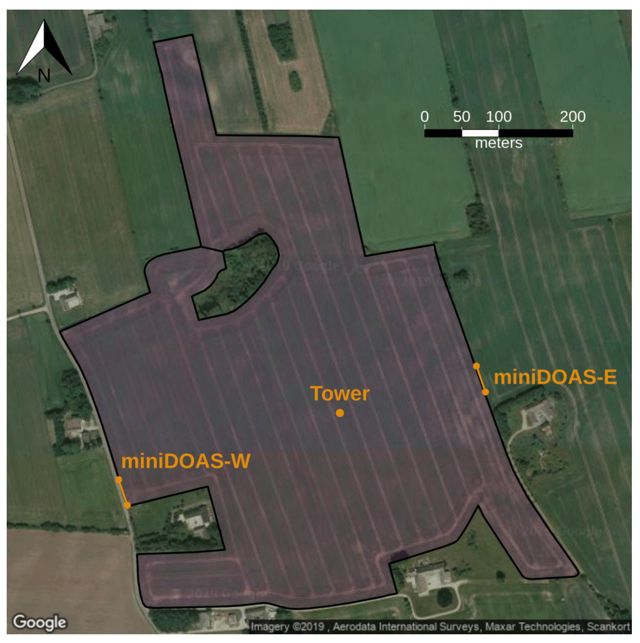
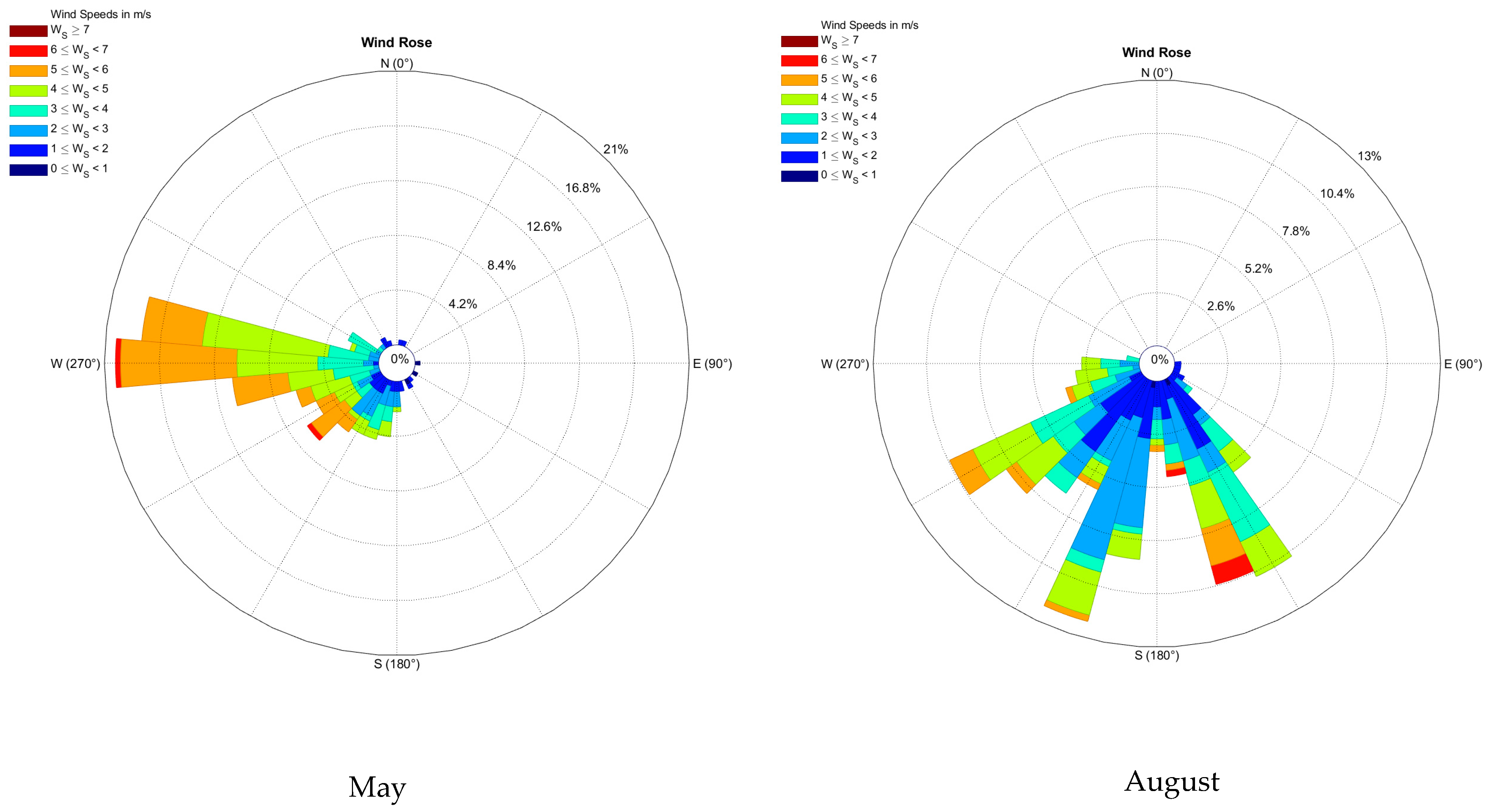
2.1. Site Description
2.2. Instrumentation
2.3. Estimation of NH3 Emission Rates
- (1)
- measurement of the vertical NH3 flux by the AGM in combination with a flux footprint model and
- (2)
- measurement of the NH3 concentration in combination with a concentration footprint model.
2.4. Aerodynamic Gradient Method
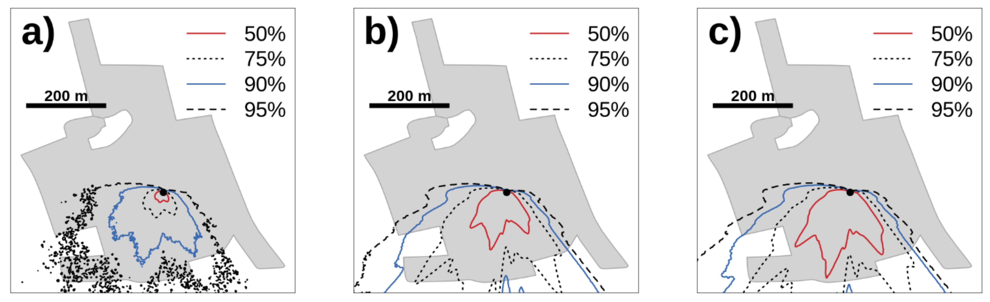
2.5. Dispersion Modeling
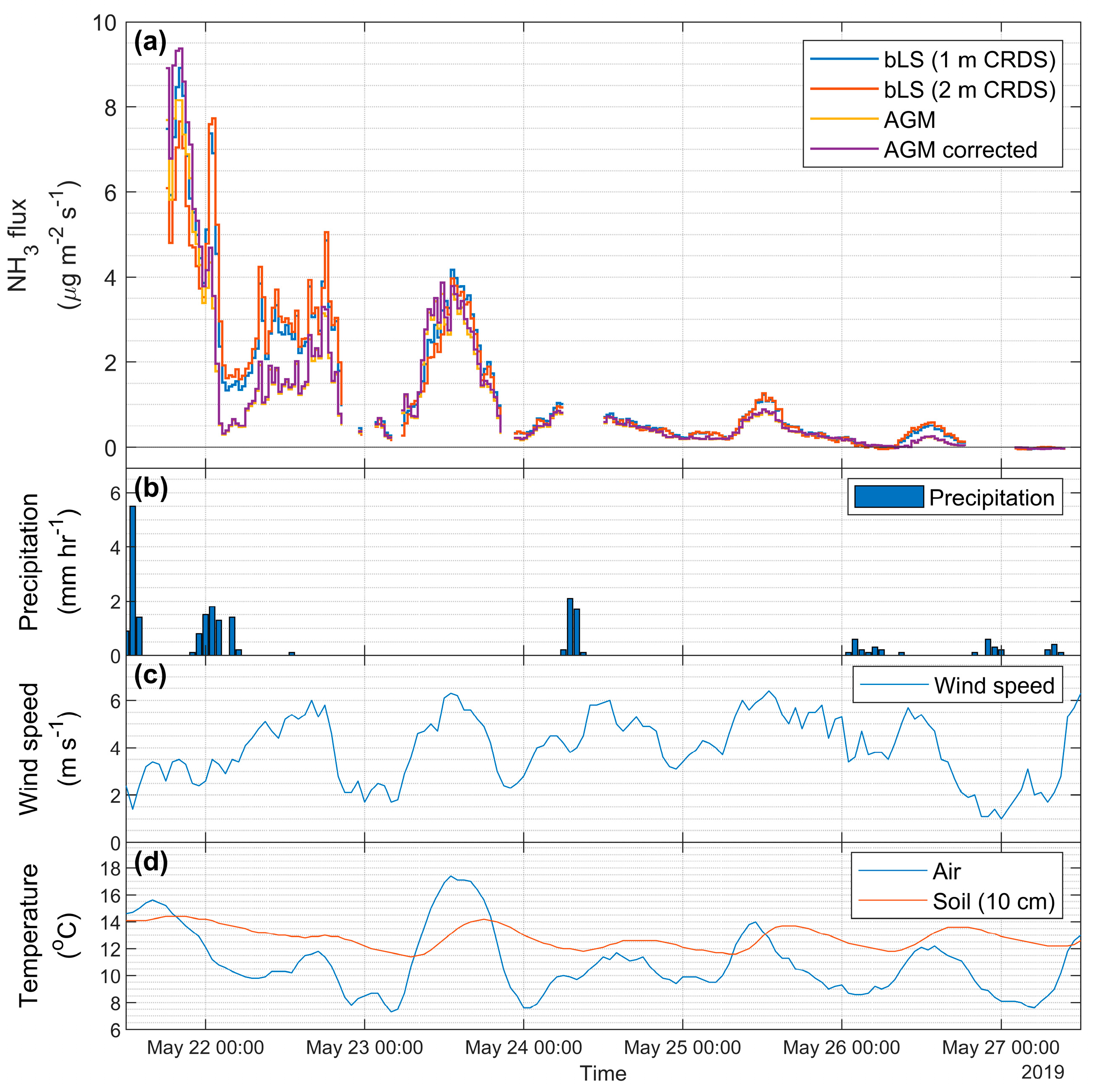
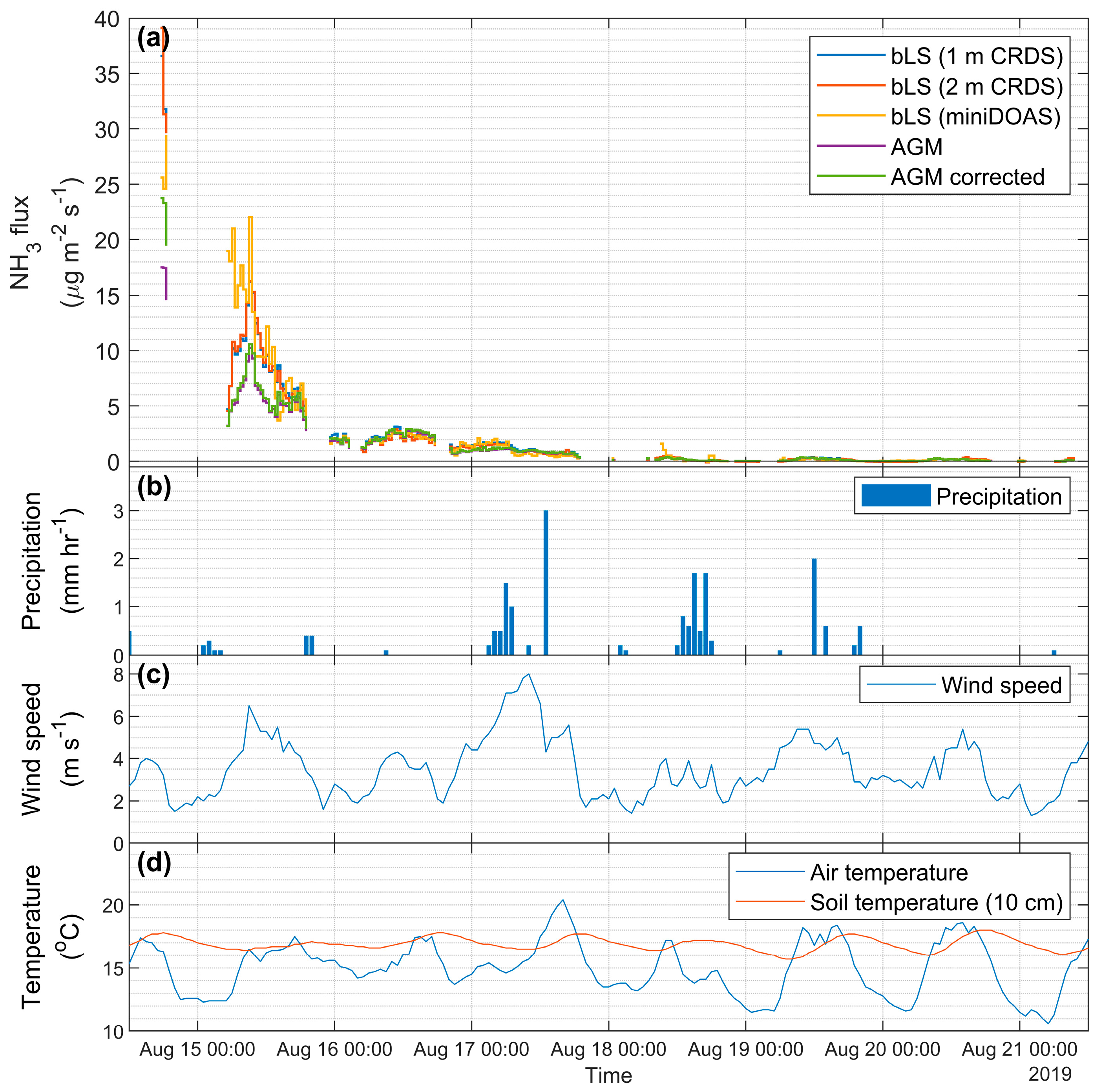
3. Results
4. Discussion
5. Conclusions
Author Contributions
Funding
Data Availability Statement
Acknowledgments
Conflicts of Interest
References
- Glibert, P.M. Eutrophication, harmful algae and biodiversity—Challenging paradigms in a world of complex nutrient changes. Mar. Pollut. Bull. 2017, 124, 591–606. [Google Scholar] [CrossRef] [PubMed]
- Binzer, A.; Guill, C.; Rall, B.C.; Brose, U. Interactive effects of warming, eutrophication and size structure: Impacts on biodiversity and food-web structure. Glob. Chang. Biol. 2016, 22, 220–227. [Google Scholar] [CrossRef] [PubMed]
- Sheppard, L.J.; Leith, I.D.; Mizunuma, T.; Cape, J.N.; Crossley, A.; Leeson, S.; Sutton, M.A.; van Dijk, N.; Fowler, D. Dry deposition of ammonia gas drives species change faster than wet deposition of ammonium ions: Evidence from a long-term field manipulation. Glob. Chang. Biol. 2011, 17, 3589–3607. [Google Scholar] [CrossRef]
- Aneja, V.P.; Roelle, P.A.; Murray, G.C.; Southerland, J.; Erisman, J.W.; Fowler, D.; Asman, W.A.H.; Patni, N. Atmospheric nitrogen compounds II: Emissions, transport, transformation, deposition and assessment. Atmos. Environ. 2001, 35, 1903–1911. [Google Scholar] [CrossRef]
- Zhu, X.; Burger, M.; Doane, T.A.; Horwath, W.R. Ammonia oxidation pathways and nitrifier denitrification are significant sources of N2O and NO under low oxygen availability. Proc. Natl. Acad. Sci. USA 2013, 110, 6328–6333. [Google Scholar] [CrossRef] [Green Version]
- Nielsen, O.K.; Plejdrup, M.S.; Winther, M.; Mikkelsen, M.H.; Nielsen, M.; Gyldenkærne, S.; Fauser, P.; Albrektsen, R.; Hjelgaard, K.H.; Bruun, H.G.; et al. Annual Danish Informative Inventory Report to UNECE. Emission inventories from the base year of the protocols to year 2015; Aarhus University DCE — Danish Centre for Environment and Energy: Aarhus, Denmark, 2017; Available online: http://dce2.au.dk/pub/SR222.pdf (accessed on 3 December 2020).
- UNECE. Protocol to Abate Acidification, Eutrophication and Ground-level Ozone. 1999. Available online: http://www.unece.org/env/lrtap/multi_h1.html (accessed on 25 September 2019).
- Leith, I.D.; Sheppard, L.J.; Fowler, D.; Cape, J.N.; Jones, M.; Crossley, A.; Hargreaves, K.J.; Tang, Y.S.; Theobald, M.; Sutton, M.R. Quantifying dry NH3 deposition to an ombrotrophic bog from an automated NH3 field release system. Water Air Soil Pollut. Focus 2005, 4, 207–218. [Google Scholar] [CrossRef]
- Wyers, G.P.; Otjes, R.P.; Slanina, J. A continuous-flow denuder for the measurement of ambient concentrations and surface-exchange fluxes of ammonia. Atmos. Environ. 1993, 27, 2085–2090. [Google Scholar] [CrossRef]
- Sørensen, L.L.; Granby, K.; Nielsen, H.; Asman, W.A.H. Diffusion scrubber technique used for measurements of atmospheric ammonia. Atmos. Environ. 1994, 28, 3637–3645. [Google Scholar] [CrossRef]
- Hensen, A.; Nemitz, E.; Flynn, M.J.; Blatter, A.; Jones, S.K.; Sørensen, L.L.; Hensen, B.; Pryor, S.C.; Jensen, B.; Otjes, R.P.; et al. Inter-comparison of ammonia fluxes obtained using the Relaxed. Biogeosciences 2009, 6, 2575–2588. [Google Scholar] [CrossRef] [Green Version]
- Sintermann, J.; Spirig, C.; Jordan, A.; Kuhn, U.; Ammann, C.; Neftel, A. Eddy covariance flux measurements of ammonia by high temperature chemical ionisation mass spectrometry. Atmos. Meas. Tech. 2011, 4, 599–616. [Google Scholar] [CrossRef] [Green Version]
- Ferrara, R.M.; Carozzi, M.; di Tommasi, P.; Nelson, D.D.; Fratini, G.; Bertolini, T.; Magliulo, V.; Acutis, M.; Rana, G. Dynamics of ammonia volatilisation measured by eddy covariance during slurry spreading in north Italy. Agric. Ecosyst. Environ. 2016, 219, 1–13. [Google Scholar] [CrossRef]
- Brodeur, J.J.; Warland, J.S.; Staebler, R.M.; Wagner-Riddle, C. Technical note: Laboratory evaluation of a tunable diode laser system for eddy covariance measurements of ammonia flux. Agric. For. Meteorol. 2009, 149, 385–391. [Google Scholar] [CrossRef] [Green Version]
- Vaittinen, O.; Metsälä, M.; Persijn, S.; Vainio, M.; Halonen, L. Adsorption of ammonia on treated stainless steel and polymer surfaces. Appl. Phys. B 2014, 115, 185–196. [Google Scholar] [CrossRef]
- Eugster, W.; Senn, W. A cospectral correction model for measurement of turbulent NO2 flux. Bound. Layer Meteorol. 1995, 74, 321–340. [Google Scholar] [CrossRef]
- Sintermann, J.; Dietrich, K.; Häni, C.; Bell, M.; Jocher, M.; Neftel, A. A miniDOAS instrument optimised for ammonia field measurements. Atmos. Meas. Tech. 2016, 9, 2721–2734. [Google Scholar] [CrossRef] [Green Version]
- Flesch, T.K.; Wilson, J.D.; Harper, L.A.; Crenna, B.P.; Sharpe, R.R. Deducing Ground-to-Air Emissions from Observed Trace Gas Concentrations. J. Appl. Meteorol. 2004, 43, 487–502. [Google Scholar] [CrossRef] [Green Version]
- Häni, C.; Flechard, C.; Neftel, A.; Sintermann, J.; Kupper, T. Accounting for field-scale dry deposition in backward Lagrangian stochastic dispersion modelling of NH3emissions. Atmosphere 2018, 9, 146. [Google Scholar] [CrossRef] [Green Version]
- Kamp, J.N.; Häni, C.; Nyord, T.; Feilberg, A.; Sørensen, L.L. The aerodynamic gradient method: Implications of non-simultaneous measurements at alternating heights. Atmosphere 2020, 11, 1067. [Google Scholar] [CrossRef]
- Spirig, C.; Flechard, C.R.; Ammann, C.; Neftel, A. The annual ammonia budget of fertilised cut grassland—Part 1: Micrometeorological flux measurements and emissions after slurry application. Biogeosciences 2010, 7, 521–536. [Google Scholar] [CrossRef] [Green Version]
- Flesch, T.K.; Wilson, J.D.; Harper, L.A. Deducing ground-to-air emissions from observed trace gas concentrations: A field trial with wind disturbance. J. Appl. Meteorol. 2005, 44, 475–484. [Google Scholar] [CrossRef]
- Loubet, B.; Génermont, S.; Ferrara, R.; Bedos, C.; Decuq, C.; Personne, E.; Fanucci, O.; Durand, B.; Rana, G.; Cellier, P. An inverse model to estimate ammonia emissions from fields. Eur. J. Soil Sci. 2010, 61, 793–805. [Google Scholar] [CrossRef]
- Sanz, A.; Misselbrook, T.; Sanz, M.J.; Vallejo, A. Use of an inverse dispersion technique for estimating ammonia emission from surface-applied slurry. Atmos. Environ. 2010, 44, 999–1002. [Google Scholar] [CrossRef]
- Sintermann, J.; Ammann, C.; Kuhn, U.; Spirig, C.; Hirschberger, R.; Gärtner, A.; Neftel, A. Determination of field scale ammonia emissions for common slurry spreading practice with two independent methods. Atmos. Meas. Tech. 2011, 4, 1821–1840. [Google Scholar] [CrossRef] [Green Version]
- Häni, C.; Sintermann, J.; Kupper, T.; Jocher, M.; Neftel, A. Ammonia emission after slurry application to grassland in Switzerland. Atmos. Environ. 2016, 125, 92–99. [Google Scholar] [CrossRef]
- Carozzi, M.; Loubet, B.; Acutis, M.; Rana, G.; Ferrara, R.M. Inverse dispersion modelling highlights the efficiency of slurry injection to reduce ammonia losses by agriculture in the Po Valley (Italy). Agric. For. Meteorol. 2013, 171–172, 306–318. [Google Scholar] [CrossRef]
- Møller, H.B.; Nielsen, K.J. Biogas Taskforce: Udvikling og Effektivisering af Biogasproduktionen i Danmark DCA Rapport nr. 77; Aarhus University DCA - Nationalt Center for Fødevarer og Jordbrug, Foulum, Denmark: Tjele, Denmark, 2016; Available online: https://pure.au.dk/portal/da/persons/henrik-bjarne-moeller(a2eda86a-cdac-4996-8db0-3cecfe51be12)/publications/biogas-taskforce(a37f2aac-aa93-4f1b-b644-051ba91b2421)/export.html (accessed on 3 December 2020).
- Kamp, J.N.; Chowdhury, A.; Adamsen, A.P.S.; Feilberg, A. Negligible influence of livestock contaminants and sampling system on ammonia measurements with cavity ring-down spectroscopy. Atmos. Meas. Tech. 2019, 12, 2837–2850. [Google Scholar] [CrossRef] [Green Version]
- Businger, J.A. Evaluation of the accuracy with which dry deposition can be measured with current micrometeorological techniques. J. Clim. Appl. Meteorol. 1986, 25, 1100–1124. [Google Scholar] [CrossRef] [Green Version]
- Kljun, N.; Calanca, P.; Rotach, M.W.; Schmid, H.P. A simple two-dimensional parameterisation for Flux Footprint Prediction (FFP). Geosci. Model Dev. 2015, 8, 3695–3713. [Google Scholar] [CrossRef] [Green Version]
- Edwards, G.C.; Rasmussen, P.E.; Schroeder, W.H.; Wallace, D.M.; Halfpenny-Mitchell, L.; Dias, G.M.; Kemp, R.J.; Ausma, S. Development and evaluation of a sampling system to determine gaseous Mercury fluxes using an aerodynamic micrometeorological gradient method. J. Geophys. Res. D Atmos. 2005, 110, 1–11. [Google Scholar] [CrossRef] [Green Version]
- Dyer, A.J.; Hicks, B.B. Flux-gradient relationships in the constant flux layer. Q. J. R. Meteorol. Soc. 1970, 96, 715–721. [Google Scholar] [CrossRef]
- Flesch, T.K. The Footprint for Flux Measurements, from Backward Lagrangian Stochastic Models. Bound. Layer Meteorol. 1996, 78, 399–404. [Google Scholar] [CrossRef]
- Flesch, T.K.; Wilson, J.D.; Harper, L.A.; Crenna, B.P. Estimating gas emissions from a farm with an inverse-dispersion technique. Atmos. Environ. 2005, 39, 4863–4874. [Google Scholar] [CrossRef]
- Hafner, S.D.; Pacholski, A.; Bittman, S.; Burchill, W.; Bussink, W.; Chantigny, M.; Carozzi, M.; Génermont, S.; Häni, C.; Hansen, M.N.; et al. The ALFAM2 database on ammonia emission from field-applied manure: Description and illustrative analysis. Agric. For. Meteorol. 2018, 258, 66–79. [Google Scholar] [CrossRef] [Green Version]
- Kljun, N.; Kormann, R.; Rotach, M.W.; Meixer, F.X. Comparison of the Langrangian footprint model LPDM-B with an analytical footprint model. Bound. Layer Meteorol. 2003, 106, 349–355. [Google Scholar] [CrossRef]
- Bell, M.; Flechard, C.; Fauvel, Y.; Häni, C.; Sintermann, J.; Jocher, M.; Menzi, H.; Hensen, A.; Neftel, A. Ammonia emissions from a grazed field estimated by miniDOAS measurements and inverse dispersion modelling. Atmos. Meas. Tech. 2017, 10, 1875–1892. [Google Scholar] [CrossRef] [Green Version]
- Sutton, M.A.; Milford, C.; Nemitz, E.; Theobald, M.R.; Hill, P.W.; Fowler, D.; Schjoerring, J.K.; Mattsson, M.E.; Nielsen, K.H.; Husted, S.; et al. Biosphere-atmosphere interactions of ammonia with grasslands: Experimental strategy and results from a new European initiative. Plant Soil 2001, 228, 131–145. [Google Scholar] [CrossRef]
- Laubach, J.; Kelliher, F.M. Measuring methane emission rates of a dairy cow herd by two micrometeorological techniques. Agric. For. Meteorol. 2004, 125, 279–303. [Google Scholar] [CrossRef]
- Beauchamp, E.G.; Kidd, G.E.; Thurtell, G. Ammonia volatilization from liquid dairy cattle manure in the field. Can. J. Soil Sci. 1982, 62, 11–19. [Google Scholar] [CrossRef]
- Sommer, S.G.; Génermont, S.; Cellier, P.; Hutchings, N.J.; Olesen, J.E.; Morvan, T. Processes controlling ammonia emission from livestock slurry in the field. Eur. J. Agron. 2003, 19, 465–486. [Google Scholar] [CrossRef]
- Hansen, M.N.; Sommer, S.G.; Hutchings, N.J.; Sørensen, P. Emission factors for calculation of ammonia volatilization by storage and application of animal manure. J. Agric. Sci. 2018, 156, 1070–1078. [Google Scholar] [CrossRef] [Green Version]
- Nelson, A.J.; Lichiheb, N.; Koloutsou-Vakakis, S.; Rood, M.J.; Heuer, M.; Myles, L.T.; Joo, E.; Miller, J.; Bernacchi, C. Ammonia flux measurements above a corn canopy using relaxed eddy accumulation and a flux gradient system. Agric. For. Meteorol. 2019, 264, 104–113. [Google Scholar] [CrossRef]
- Vesala, T.; Kljun, N.; Rannik, Ü.; Rinne, J.; Sogachev, A.; Markkanen, T.; Sabelfeld, K.; Foken, T.; Leclerc, M.Y. Flux and concentration footprint modelling: State of the art. Environ. Pollut. 2008, 152, 653–666. [Google Scholar] [CrossRef] [PubMed]


| Measurement Period | Dry Matter (%) | Total kg N ton−1 | Kg NH4+-N ton−1 | Phosphorus (kg ton−1) | Potassium (kg ton−1) | pH | Application Rate (ton ha−1) |
|---|---|---|---|---|---|---|---|
| May | 5.35 | 3.10 | 1.80 | 0.47 | 2.06 | 7.8 | 30 |
| August | 3.31 | 2.79 | 1.62 | 0.36 | 1.78 | 7.7 | 35 |
| Method | Mean Emission (µg m−2 s−1) | |
|---|---|---|
| May | August | |
| AGM | 1.05 | 1.40 |
| AGM (footprint-corrected) | 1.13 | 1.53 |
| bLS (1-m CRDS) | 1.38 | 2.05 |
| bLS (2-m CRDS) | 1.33 | 2.00 |
| bLS (miniDOAS) | - | 2.58 |
| Method | Loss of TAN in % | |
|---|---|---|
| May | August | |
| AGM | 8.2 | 10.3 |
| AGM (footprint-Corrected) | 8.9 | 11.3 |
| bLS (CRDS 1 m) | 10.7 | 15.1 |
| bLS (CRDS 2 m) | 10.4 | 14.6 |
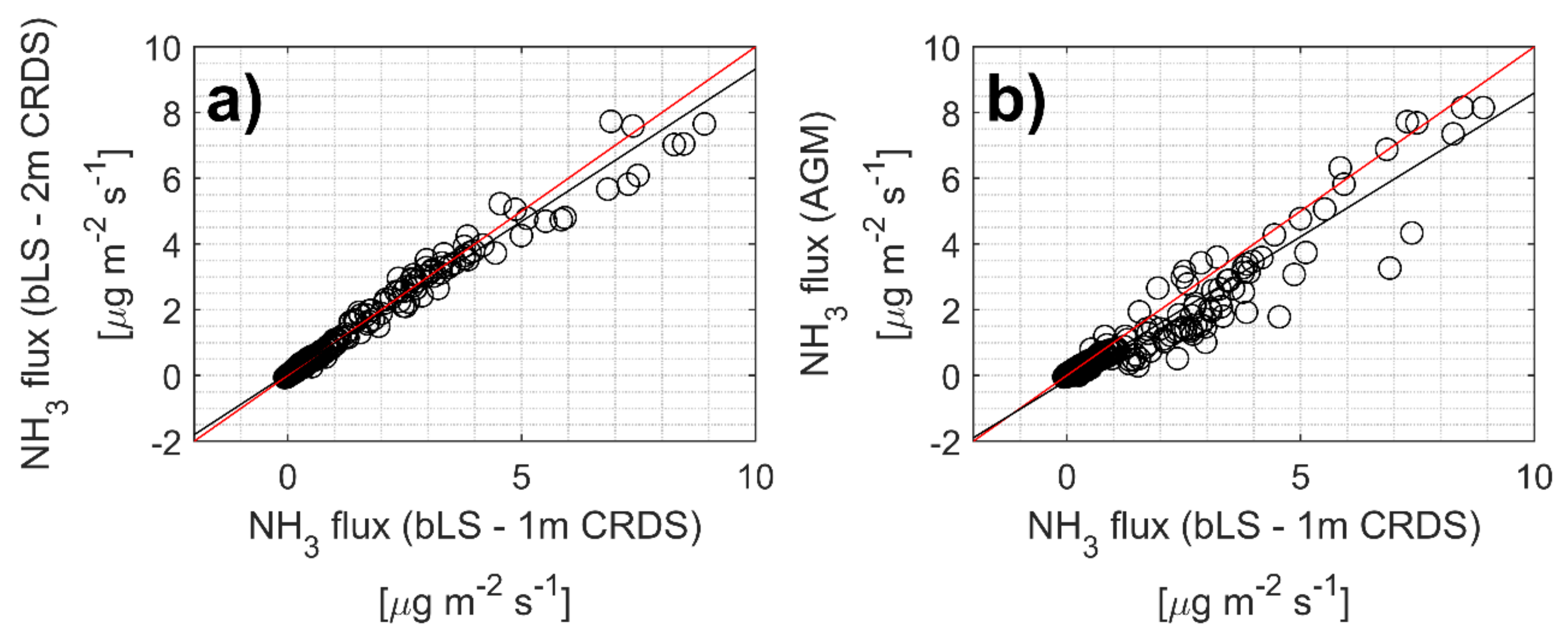
| Compared Methods for Regression | Slope | Intercept | Pearson Correlation | ||
|---|---|---|---|---|---|
| May | bLS (1-m CRDS) | bLS (2-m CRDS) | 0.93 ± 0.02 | 0.05 ± 0.02 | 0.988 |
| bLS (1-m CRDS) | AGM | 0.88 ± 0.04 | −0.15 ± 0.03 | 0.952 | |
| bLS (1-m CRDS) | AGM (fp-corrected) | 0.99 ± 0.05 | −0.22 ± 0.05 | 0.946 | |
| August | bLS (1-m CRDS) | bLS (2-m CRDS) | 1.01 ± 0.02 | −0.10 ± 0.03 | 0.999 |
| bLS (1-m CRDS) | bLS (miniDOAS) | 1.03 ± 0.13 | 0.01 ± 0.20 | 0.911 | |
| bLS (1-m CRDS) | AGM | 0.55 ± 0.03 | 0.27 ± 0.05 | 0.980 | |
| bLS (miniDOAS) | AGM | 0.51 ± 0.05 | 0.38 ± 0.07 | 0.910 | |
| bLS (1-m CRDS) | AGM (fp-corrected) | 0.70 ± 0.02 | 0.16 ± 0.03 | 0.991 | |
| bLS (miniDOAS) | AGM (fp-corrected) | 0.62 ± 0.08 | 0.25 ± 0.13 | 0.894 | |
Publisher’s Note: MDPI stays neutral with regard to jurisdictional claims in published maps and institutional affiliations. |
© 2021 by the authors. Licensee MDPI, Basel, Switzerland. This article is an open access article distributed under the terms and conditions of the Creative Commons Attribution (CC BY) license (http://creativecommons.org/licenses/by/4.0/).
Share and Cite
Kamp, J.N.; Häni, C.; Nyord, T.; Feilberg, A.; Sørensen, L.L. Calculation of NH3 Emissions, Evaluation of Backward Lagrangian Stochastic Dispersion Model and Aerodynamic Gradient Method. Atmosphere 2021, 12, 102. https://doi.org/10.3390/atmos12010102
Kamp JN, Häni C, Nyord T, Feilberg A, Sørensen LL. Calculation of NH3 Emissions, Evaluation of Backward Lagrangian Stochastic Dispersion Model and Aerodynamic Gradient Method. Atmosphere. 2021; 12(1):102. https://doi.org/10.3390/atmos12010102
Chicago/Turabian StyleKamp, Jesper Nørlem, Christoph Häni, Tavs Nyord, Anders Feilberg, and Lise Lotte Sørensen. 2021. "Calculation of NH3 Emissions, Evaluation of Backward Lagrangian Stochastic Dispersion Model and Aerodynamic Gradient Method" Atmosphere 12, no. 1: 102. https://doi.org/10.3390/atmos12010102