Article

Investigation of the Vertical Influence of the 11-Year Solar Cycle on Ozone Using SBUV and Antarctic Ground-Based Measurements and CMIP6 Forcing Data

1
Physics Faculty, Taras Shevchenko National University of Kyiv, 01601 Kyiv, Ukraine
2
Antarctica and the Global System, Australian Antarctic Division, Kingston 7050, Australia
3
School of Earth Sciences, University of Melbourne, Melbourne 3053, Australia
4
College of Physics, International Center of Future Science, Jilin University, Changchun 130012, China
5
Department of Atmosphere Physics and Geospace, National Antarctic Scientific Center, 01601 Kyiv, Ukraine
6
Department of Radio Physics of Geospace, Institute of Radio Astronomy, NAS of Ukraine, 61002 Kharkiv, Ukraine
*
Author to whom correspondence should be addressed.
Atmosphere 2020, 11(8), 873; https://doi.org/10.3390/atmos11080873
Submission received: 27 July 2020 / Revised: 7 August 2020 / Accepted: 14 August 2020 / Published: 17 August 2020
(This article belongs to the Section Meteorology)

Abstract

:
The 11-year solar activity cycle in the vertical ozone distribution over the Antarctic station Faraday/Vernadsky in the Antarctic Peninsula region (65.25° S, 64.27° W) was analyzed using the Solar Backscatter Ultra Violet (SBUV) radiometer data Version 8.6 Merged Ozone Data Sets (MOD) over the 40-year period 1979–2018. The SBUV MOD ozone profiles are presented as partial column ozone in layers with approximately 3-km altitude increments from the surface to the lower mesosphere (1000–0.1 hPa, or 0–64 km). Periodicities in the ozone time series of the layer data were studied using wavelet transforms. A statistically significant signal with a quasi-11-year period consistent with solar activity forcing was found in the lower–middle stratosphere at 22–31 km in ozone over Faraday/Vernadsky, although signals with similar periods were not significant in the total column measurements made by the Dobson spectrophotometer at the site. For comparison with other latitudinal zones, the relative contribution of the wavelet spectral power of the quasi-11-year periods to the 2–33-year period range on the global scale was estimated. While a significant solar activity signal exists in the tropical lower and upper stratosphere and in the lower mesosphere in SBUV MOD, we did not find evidence of similar signals in the ozone forcing data for the Coupled Model Intercomparison Project Phase 6 (CMIP6). In the extratropical lower–middle stratosphere and lower mesosphere, there is a strong hemispheric asymmetry in solar activity–ozone response, which is dominant in the Southern Hemisphere. In general, the results are consistent with other studies and highlight the sensitivity of ozone in the lower–middle stratosphere over the Antarctic Peninsula region to the 11-year solar cycle.

1. Introduction

While ozone is only a minor constituent in the terrestrial atmosphere, it is of great importance for the natural state of the biosphere by absorbing near-ultraviolet solar radiation with wavelengths less than 300 nm [1]. The vertical profile of stratospheric ozone is characterized by a sharp altitudinal maximum of photochemical origin at heights of ~20 km [2,3,4], with approximately 90% of the total ozone column (TOC) confined to the stratosphere. The meridional ozone distribution shows a minimum at low latitudes, with a generally positive gradient in TOC towards higher latitudes [3]. The exceptions to this are the seasonally dependent meridional gradients of ozone in the polar regions, which can become negative when the polar vortices form. The dynamical barrier due to the strong zonal wind at the vortex edge region leads to significant ozone depletion in the ozone hole over the Antarctica in austral spring [2,5,6] and less commonly over the Arctic in boreal winter–spring [7,8,9]; see, e.g., [10] for the Arctic ozone hole 2020.
The concentration of ozone in the Earth’s atmosphere depends on several factors, which can be categorized as being either chemical or dynamical in nature [2,3]. The first category is connected with chemical reactions that create or destroy ozone, aspects of which are dependent on the flux of solar ultraviolet (UV) radiation [11]. The stratospheric ozone concentration is affected by variations in the concentration of different atmosphere constituents, including chlorofluorocarbons and related ozone-depleting substances [11,12] and chemical radicals, such as NO and OH [13], as well as changes in solar radiation resulting from variations in insolation and solar activity [14].
In the second category, dynamical processes associated with the Brewer–Dobson circulation (BDC) [15,16] and the propagation of planetary waves [17] are most important in setting the large-scale distribution of ozone. A transitional zone separating altitudes dominated by chemical (upper stratosphere) and dynamical (lower stratosphere) processes lies near the 16–10 hPa level [18]. The two stratospheric layers differ in the ozone photochemical lifetime, which is short (from a few hours to a day) and long (from a few days to several months), respectively [19].
Solar UV radiation exhibits changes associated with sunspots and the 11-year solar activity cycle [20], with variability on the order of 1% in the 250–300-nm wavelength range relevant to ozone photochemistry in the upper stratosphere [21,22]. The longest series of solar activity observations relates to sunspots [23], which are the most noticeable elements of the solar photosphere. Hitherto, sunspot numbers are among the main indices of solar activity, with clear advantages in simplicity of calculation and the large duration of their series. The solar radio emission at the 10.7-cm wavelength (F10.7), which has been measured since the 1940s [24,25], is well correlated with sunspot numbers and UV variations and is used as a reliable proxy for solar activity in atmospheric models [26].
Studies of the dependence of total ozone on solar activity have a long history ([27,28,29,30,31,32], and references therein). The solar activity component in the tropical total ozone column is confirmed to have a relatively small amplitude (1–2% of the 1964–1994 mean) with an increase of the total ozone column towards the solar cycle maximum [32]. According to the Solar Backscatter Ultra Violet (SBUV) and SBUV/2 radiometers data in the period 1979–1993, most (about 85%) of the 1.5–2% solar cycle variation of the global mean total ozone column occurs in the lower stratosphere at altitudes <28 km [33]. Herewith, a partial contribution from the upper stratosphere was noted, with no contribution from the middle stratosphere.
Change in the rate of ozone dynamical transport (in the rate of photochemical production of ozone) between the solar minimum and maximum may contribute to ozone change in the lower (upper) stratosphere [33]. In the midlatitudes, ozone anomalies established in the wintertime buildup due to ozone transport persist through summer until the end of the following autumn, when transport decreases and photochemical loss dominates, and then are rapidly erased once the next winter’s buildup begins [18,34]. This means that each year can be considered as independent of the annual mean ozone content [34], which simplifies the diagnostics of the possible effects of the 11-year solar cycle. However, each season may have a different sensitivity to ozone photochemistry associated with solar radiation.
Greater changes are expected at the lowest latitudes where the mean flux of solar radiation is largest [35]. Due to the dominant photochemical influence on ozone in the upper stratosphere, the changes in solar radiation are most apparent in this stratospheric layer [36]. As described by Isaksen et al. [37], peak ozone changes due to the solar cycle are attributed to heights near 40 km. An average middle atmospheric ozone increase of the order of 2% from the solar minimum to solar maximum was noted by Calisesi and Matthes [38]. In addition to the upper stratosphere response, a tropical lower-stratospheric response exists, which is produced mainly by a solar-induced modulation of the BDC [39]. Such modulation implies a reduction of Rossby wave forcing, a weakening of the BDC, and an increase in tropical lower-stratospheric ozone and temperature near the solar maximum [39]. The 11-year ozone response in the tropical lower stratosphere at about 30–50 hPa was also found by Bordi et al. [40] using ERA-Interim reanalysis data.
Gruzdev [41] found three altitudinal maxima of the ozone–solar cycle dependence in the stratosphere using SBUV and SBUV/2 data for the 1978–2003 period, which covered two full solar cycles. With spectral, cross-spectral, and regression methods, the altitude maxima of ozone sensitivity to the 11-year solar cycle were found near the stratopause (50–55 km) and in the middle (35–40 km) and lower (below 25 km) stratosphere. According to Gruzdev [41], the ozone response in the polar regions in winter and spring is about 10% near the stratopause (over the Arctic) and in the lower stratosphere (over the Antarctic). Recent studies suggest a decrease in the magnitude of the solar activity–ozone response in the tropical upper stratosphere to ~1% relative to an earlier estimate [42,43].
There is a pronounced interhemispheric asymmetry in the solar activity response of stratospheric ozone. The largest response occurs at 65° S in the Southern Hemisphere and at about 30° N in the Northern Hemisphere [33]. The asymmetry towards the summer hemisphere for both December–February (DJF, the Southern Hemisphere) and June–August (JJA, the Northern Hemisphere) suggests an origin involving a solar modulation of the BDC [39] because the upwelling branch of the BDC is limited to low and subtropical latitudes and is also shifted somewhat toward the summer hemisphere. The magnitude of the interhemispheric asymmetry also varies with season as was noted by Soukharev and Hood [44] and Tourpali et al. [45].
Other factors are also involved in the dependence of ozone on solar forcing. It is established that polar ozone in the middle and upper stratosphere varies from year to year due to energetic particle precipitation related to solar variability and such events are particularly frequent around the maximum of the solar cycle [46]. Additionally, the 11-year solar cycle effects in the long-term recovery of ozone depletion have been noted [47,48]. Through the absorption of UV radiation by ozone, solar activity–ozone response impacts the stratospheric temperature distribution and, consequently, circulation and climate [49,50]. The uncertainties regarding solar-induced variability in observed ozone related to the type of data and/or analysis, the length of data records, and the time periods under investigation are discussed [51,52].
As an ozone measurement site, the Antarctic station Vernadsky, Ukraine (the former British Antarctic Survey station Faraday in the Antarctic Peninsula) takes a unique position during the austral spring months. The station is usually located in the region of zonal ozone minimum and frequently falls on the edge of the ozone hole (Figure 1; see, e.g., [5]). Total ozone measurements with a Dobson spectrophotometer at Faraday/Vernadsky have been carried out from the 1950s, spanning almost 70 years. Being among the longest data series in the high southern latitudes, they are useful to analyze the local variability of the total ozone on different time scales, including long-term tendencies. The data are typical for the Antarctic region in terms of decadal changes, in particular exhibiting a sharp decrease in the spring ozone values during the 1980s–1990s with subsequent stabilization [4,6,11]. The long-term shift of the zonal ozone minimum in the Atlantic sector also contributed to decadal-scale ozone change in the Faraday/Vernadsky region [53,54].
Less studied in this region is the effect of periodic changes in ozone associated with the 11-year cycle of the solar activity. In view of the existing research gap, the long record of total column measurements from Faraday/Vernadsky has been used together with total column and height-resolved measurements from the SBUV data set to study the role of the solar activity component in the local variability of ozone over the site. After summarizing the data sets in Section 2, the influence of solar activity on ozone variability over Faraday/Vernadsky is compared with the solar activity–ozone response in zonal means over both hemispheres in Section 3. In Section 4, the results are discussed, followed by summarizing the conclusions in Section 5.

2. Data and Methods

The vertical distribution of ozone is studied with data from the SBUV series of satellite instruments, which have provided measurements from 1970 [56]. These data are separated by altitude into 21 layers (each layer being ~3 km thick) covering the troposphere, stratosphere, and lower mesosphere. A sequence of the SBUV layers is determined as p k = 1013.25 · 10 0.2 ( k 1 ) , where pk corresponds to the layer k bottom pressure in hPa. The layers 1–16 (L1–L16) between the surface and the stratopause (0 km to ~50 km) are considered at the bottom pressure levels 1013, 639, 403 … 1 hPa. The layer 21 is referred to as the top of the atmosphere in zonal means and as the 0.1 hPa pressure level (64 km) in overpass data. The SBUV Version 8.6 Merged Total and Profile Ozone Data Sets (MOD) are available at [57]. The data from BUV, SBUV, SBUV/2 onboard Nimbus-4, Nimbus-7, NOAA-9, NOAA-11, NOAA-14, NOAA-16, NOAA-17, NOAA-18, NOAA-19, and measurements of Suomi NPP-OMPS are collected to create the data set. Despite some uncertainties in solar activity– ozone response, particularly in the upper stratosphere, the SBUV MOD (for simplicity, hereafter referred to as ‘SBUV’) data is favorable for diagnosing effects of the solar cycle [42]. This has minimal gaps from 1979, and therefore this part of the time series until 2018 is predominantly considered.
Because information on the ozone distribution from the SBUV instrument is obtained by solar backscattered ultraviolet radiation, data are absent in the polar night regions. This provides a restriction on the analysis of seasonal changes at high latitudes. Moreover, for technical reasons, while the satellites are on Sun-synchronous orbits with an inclination near 98°, the data are only available equatorward of 80° latitude. The SBUV database consists of ozone overpass data for the individual ground-based stations. The overpasses over Faraday/Vernadsky (65.25° S, 64.27° W; Antarctic Peninsula in western Antarctica) are used here. Since the SBUV zonal means include only the sum of layers 1–8, the version of the aggregated overpasses at [58] has been used. The latter contain data for all 21 layers.
The 40-year climatology (1979–2018) of the vertical ozone distribution over Faraday/Vernadsky from the SBUV layer ozone column is shown in Figure 2a. Here, the units shown are Dobson Units (DU), where 1 DU corresponds to a gas layer with the thickness in 0.01 mm at standard temperature and pressure (0 °C, 1013 hPa) or 2.687 × 10²⁰ molecules m−2 [59]. The layer sequence L1 to L16 (0–50 km) is presented. For the full thickness of the multiple layers, the bottom (top) pressure and height of the lower (upper) layer are indicated hereinafter. Maxima of 45 and 41 DU in partial column ozone are observed in layers L7 and L8, respectively. The corresponding heights of 19–25 km are typical for the maximum in the vertical ozone profile observed at Antarctic stations [2]. L7 and L8 contribute ~30% to the total ozone column, which is 285 DU in the sum of L1–L21, in accordance with ground-based observation of the total ozone at Vernadsky [60]. Ozone minima are in the lowermost troposphere (6–7 DU in L1 and L2, 0–7 km) and the upper stratosphere (1–2 DU, L15 and L16, 43–50 km).
The total ozone time series from the Faraday/Vernadsky Dobson spectrophotometer and other sources are compared in Figure 2b. Pearson’s correlation coefficients r are shown in Table 1. Data sets from SBUV overpasses, the European Centre for Medium-Range Weather Forecasts 5th reanalysis (ERA5; [61,62]), and the Modern-Era Retrospective analysis for Research and Applications Version 2 reanalysis (MERRA2; [63,64]) are all highly correlated with the Dobson spectrophotometer data with r = 0.8–0.9. The Dobson and SBUV data correlate with r = 0.92. Lower, but significant at the 95% confidence level, is the correlation between Dobson and the Coupled Model Intercomparison Project Phase 6 (CMIP6; [65,66]) ozone forcing data (r = 0.5–0.7). CMIP6 overestimates the other data sets by 30–40 DU (11–14%), while the Dobson spectrophotometer and SBUV have identical climatological means for the 1979–2018 period: 276.9 ± 14.2 DU and 276.7 ± 15.2 DU, respectively (±standard deviation), and coincide in long-term trends (not shown).
This is consistent with an absence of time-dependent differences between SBUV and ground-based instruments noted earlier [67,68]. Ball et al. [52] propose new artifact-corrected ozone composites (BASICv2) that best represent the historical upper stratospheric solar variability, and note those based on SBUV alone should not be used. Upper stratospheric ozone in this analysis makes up only a small part of the ozone profile (Figure 2a) and the main conclusions presented here are based on the SBUV data in the lower and middle stratosphere.
To characterize solar activity, the information on sunspot numbers from [69] and for F10.7 from [70,71] was used. In both cases, the monthly mean data are analyzed.
Periodicity in both solar indices and layer ozone content is studied using the Morlet wavelet transform [72]. This approach allows analysis of the non-stationary signal with variable frequencies. This is significant for both solar cycles of changing duration and less evident variations of the ozone content at different altitudes. The wavelet transform is realized as:
F ( τ , s ) = 1 s f ( t ) ψ ( t τ s ) d t ,
where τ is the time shift and s is the scale parameter. The Morlet function is used as:
ψ ( t ) = e t 2 / 2 · e i a t ,
where a is equal to 5 or 6, with time t in years in this study. Wavelet transform with the real part of this function was also considered. The scale parameter is connected with period T by the relation [72]:
T = 4 π s a + 2 + a 2 ,
where approximately T = 2 π s a . From Equation (3), T/s is 1.03 for a = 6 or 1.23 for a = 5.
To estimate a possible latitudinal and seasonal dependence of periods close to 11 years, the ratio of wavelet transform intensity in the range of 10–12 years, observed historically in the solar cycle [23], to the total intensity over the range of 2–33 years was calculated. The wavelet power spectrum was retrieved using the annual mean data and time scales starting from 2 years were analyzed. The geometric progression with the common ratio 21/4 was used, as a result, time scales for the periods of 2 years, 2 × 21/4 years, … were considered. The period sequence obtained from (3) is approximately 2.1, 2.5, 2.9, 3.5, 4.1, 4.9, 5.8, 6.9, 8.3, 9.8, 11.7, 13.9, 16.5, 19.7, 23.4, 27.8, and 33.1 years. In calculation of the wavelet intensity ratio, the periods 9.8 and 11.7 years were compared with the rest of the listed values.

3. Results

3.1. Solar Cycles in Sunspot Numbers and 10.7 cm Solar Flux

As noted in the introduction, the main solar activity cycle is characterized by a period of nearly 11 years. This is established from data on sunspot numbers or solar flux at the 10.7-cm wavelength (Figure 3). In the minimum of the solar cycle, sunspots may be totally absent. Solar cycles have consecutive numbers starting at the cycle maximum close to the year 1750 [23]. The maximum of the last cycle 24 was weaker than a majority of the previously identified cycles and its minimum was reached in 2019–2020 (Figure 3). Specifically, the maximum of the cycle 24 was lower than the maximum of the cycle 20 (the late 1960s), which was characterized by the minimal sunspot numbers and 10.7 cm solar flux from the middle of the 20th century. At the maxima of the cycles 18, 19, and 21–23, sunspot numbers exceeded 200 with the historical peak values above 300 in the cycle 19 (maximum in 1957, see Figure 3).
The Morlet wavelet transform clearly identifies the 11-year solar cycle in the data of sunspot numbers (Figure 4), which is almost identical in F10.7 (not shown). The cycle length varies from 10 to 12 years relative to the 11-year period (dashed and solid lines in Figure 4a and dashed horizontal lines in Figure 4c). The lower intensity of the cycle 24 seen from Figure 3 is also represented in the wavelet transform in Figure 4a,b.
The solar cycle signal is statistically significant at the 95% confidence level and covers the period range of 8–13 years (inside black contour in Figure 4b and to the right of dashed curve in Figure 4c).

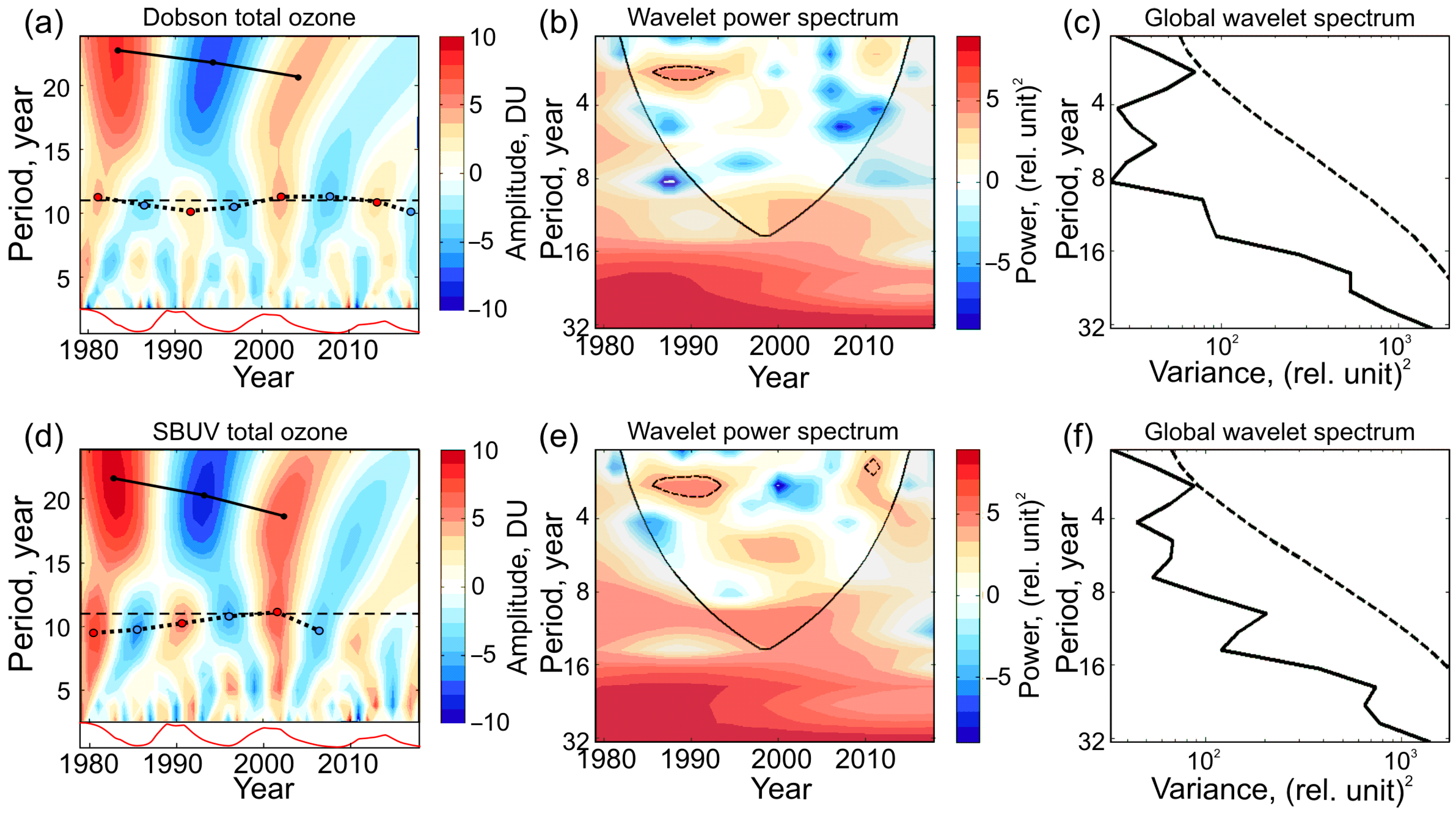
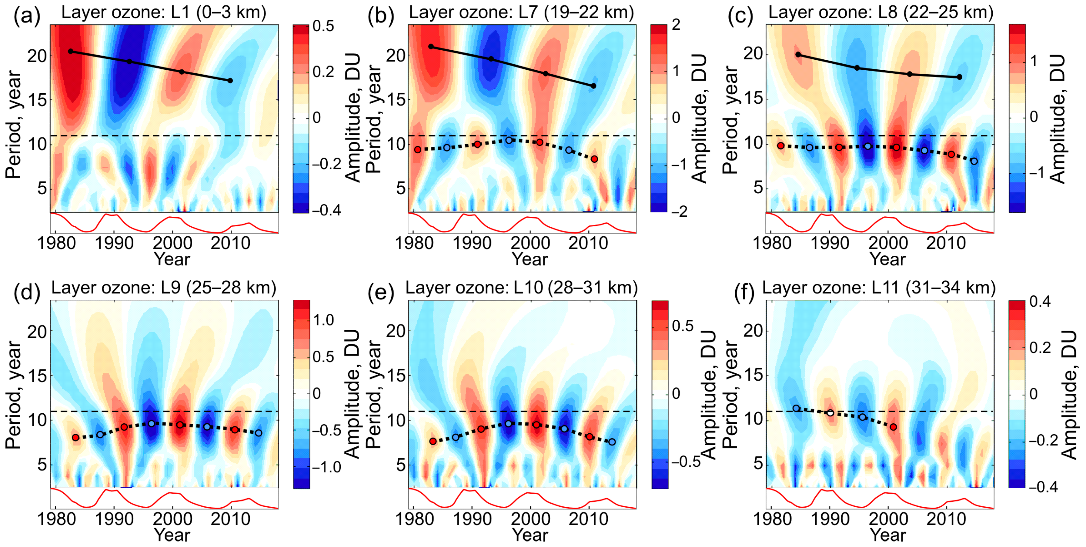
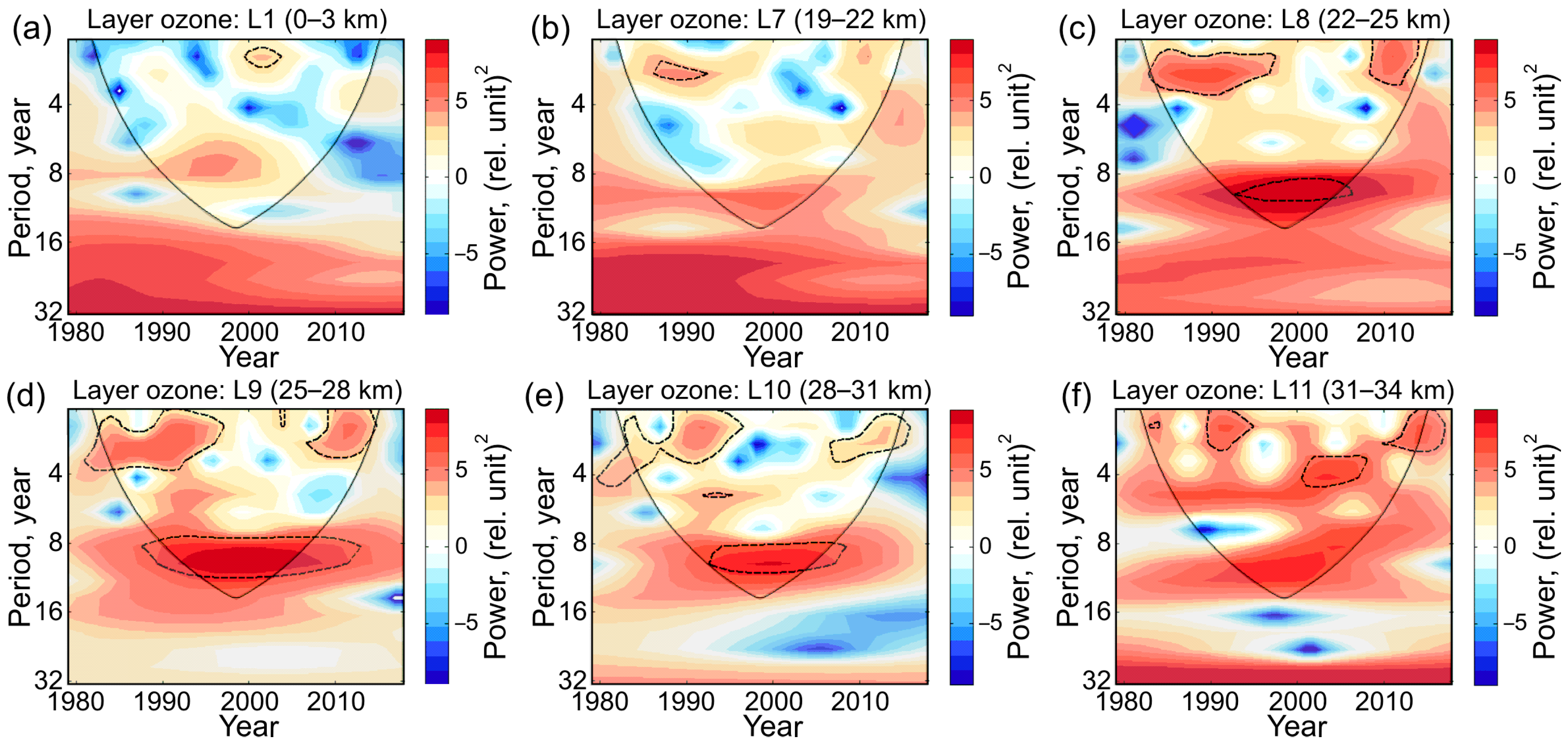
3.2. Periodicity in Ozone Variations

First, the solar cycle response in total ozone over Faraday/Vernadsky was examined (Figure 5). The most intense signal in wavelet amplitude is the 18–22-year periodicity in both the Dobson spectrophotometer and SBUV data (solid lines in Figure 5a,d, respectively). A very weak signal is near the 11-year period (dotted curves), but it is in a range of 10–11 years that closely corresponds to the solar cycle. There is a close similarity of the decadal oscillations in the Dobson and SBUV total ozone. There is also a general correspondence between the maxima and minima in the 11-year solar cycle (red curve at the bottom of Figure 5a,d) and in total ozone (red and blue circles, respectively). At the 20–22-year periods, the phase of total ozone oscillation lags the 21st and 23rd solar cycles (near 1980 and 2000, see Figure 3) by a few years. However, wavelet power spectra do not reveal significant signals at either 11-year or quasi-22-year periods (Figure 5b,e). An episodic appearance of quasi-biennial periods significant at the 95% confidence level is seen around 1990. The global wavelet for the entire time series 1979–2018 in Figure 5c,f did not show any significant periods.
Second, the results of the wavelet amplitude analysis in the SBUV layer ozone over Faraday/Vernadsky are presented. As seen from Figure 6, the large-amplitude periodicity close to 11 years (dotted curves) is observed only in the lower stratosphere (L8, 22–25 km; Figure 6c) and middle stratosphere (L9 and L10, 25–31 km; Figure 6d,e). These layers correspond to the upper part of the vertical ozone profile above its maximum (Figure 2) and contain 33% of the total ozone column. Note that the wavelet peaks in Figure 6c–e (red and blue circles) show somewhat shorter periods of 8–10 years than in the real solar cycles (red curve at the bottom of each plot). Because of the difference in periodicity, the ozone response shifts in phase with respect to the solar cycle (compare time shift of red–blue circles at the peak wavelet amplitude in ozone relative to the maxima and minima of the solar cycle on red curves). Because of this phase shift, the ozone cycle lags (leads) the solar cycle in the first half (at the end) of the time series (Figure 6c–e). The most coincident in time are the maxima in the ozone and sunspot number of the 23rd solar cycle (near 2000).
There is a fairly strong signal at 18–22-year periods in the troposphere (~0–3 km, L1) and in the lower stratosphere (19–25 km, L7 and L8, marked by solid lines in Figure 6a–c). This signal appears to be associated with the 22-year Hale (magnetic) cycle [23,73]. Wavelet transforms for the intermediate L2–L6 in the troposphere–lowermost stratosphere at altitudes ~3–19 km demonstrate behavior similar to that for L1 in Figure 6a (not shown). The quasi-22-year solar cycle signal rapidly weakens with height and disappears above 25 km (at L9 and higher, Figure 6d–f).
Third, Figure 7 demonstrates periodicity in the wavelet power spectra for the ozone over Faraday/Vernadsky in the same layers L1 (0–3 km) and L7–L11 (19–34 km), as in Figure 6. The 95% significance level calculated supposing lag-1 autocorrelation as 0.7 is shown by dashed contours. The cone of influence is highlighted in a lighter shade.
In correspondence with Figure 6c–e, the most intense periods close to 11 years are in the lower and middle stratosphere in the layers 8–10 (22–31 km) and they are statistically significant at the 95% confidence level (Figure 7c–e). Considering the results of Figure 6, ozone at 22–31 km over Faraday/Vernadsky increases near the solar cycle maximum, although with some phase shift noted above. The large-amplitude periods of 20–22 years do not reach statistical significance in the wavelet power spectra not only at the 95% level (Figure 7a,b) but also at the 90% level (not shown). Note that the statistically significant periods of 2–4 years appear occasionally in the wavelet power spectra in different layers.
In the troposphere (Figure 6a and Figure 7a) and upper stratosphere at 34–50 km (L12–L16, not shown), the 11-year signal is not detected. In general, the presence of the 11-year solar cycle in ozone over Faraday/Vernadsky is reliably established in the lower and middle stratosphere at 22–31 km (L8–L10, Figure 7c–e).

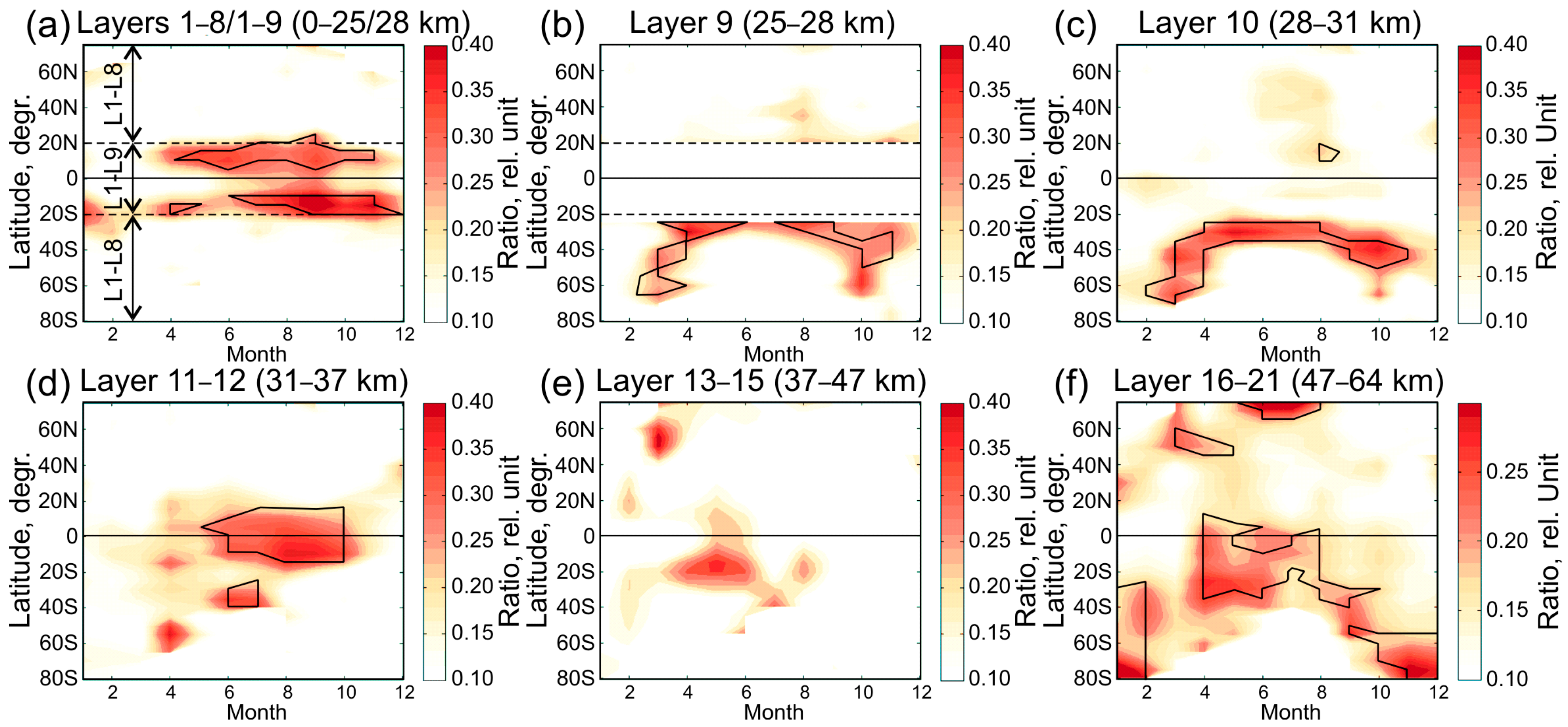
3.3. Zonal Mean Response

Next, the dependence of the solar cycle–ozone response on the latitude, altitude, and month is examined (Figure 8). This part of the analysis was carried out using the 5-degree zonal means of the SBUV ozone profile. The presence of periods close to 11 years was estimated as the relative part of the wavelet transform intensity contributed by the periods of 10–12 years into the intensity of the entire range of periods of 2–33 years (see Section 2 and Section 3.1). The discrete wavelet transform was carried out by taking the ratio of the intensity sum for 9.8 and 11.7 years to the sum of all periods from 2.1 to 33.1 years. The statistical significance was calculated separately for every period value from the global wavelet analogously to Figure 4c. This calculation does not have a one-to-one correspondence between the significance and intensity ratio. Therefore, parts of the plots with the low ratio can sometimes be significant, such as, for example, in L10 near 10° N in August (Figure 8c).
Note that the zonal mean SBUV data at [57] has latitudinal limitation in the lower layers: L9 (25–28 km) and the sum of the L1–L8 (0–25 km) layers are defined poleward of 20° only and the sum of L1–L9 (0–28 km) is defined equatorward of 20° only. Figure 8a combines the data of the 0–25 km layer poleward of 20° and the 0–28 km layer, equatorward of 20°, as indicated by the signed arrows. Besides, the high SH latitudes in austral winter are not presented in the SBUV data.
It is seen from Figure 8a that (i) the maximum contribution of the solar cycle in L1–L9 is concentrated in the tropical latitudes 20° S–20° N and (ii) seasonal change shows an insignificant contribution in February–March. No noticeable manifestations of the solar cycle in Figure 8a are visible poleward of 20° S and 20° N, where L1–L8 (0–25 km) layers are presented. This indicates that, at the altitudes 0–25 km, which covers the troposphere and includes the lower-stratospheric ozone maximum at 16–25 km (L6–L8, Figure 2a), the solar activity–ozone response is limited to the tropics.
The layers L9 and L10 (25–31 km) are the lowest in which solar cycle signal appears in the extratropics, but it prevails in the SH (Figure 8b,c). At the same time, the 11-year solar cycle signal in the tropics almost disappears at L10 (28–31 km, Figure 8c) and intensifies again above (Figure 8d–f). This weakening of the solar signal is consistent with the known double-peak structure of the 11-year solar cycle response in the tropical stratosphere ozone discussed in Section 4.
In addition to vertical irregularity, there is latitudinal inhomogeneity in the appearance of the solar cycle in the ozone data. Hemispheric asymmetry of the solar activity–ozone response in the middle and upper stratosphere is apparent (Figure 8b–f). It is seen also that the seasonal maximum of the response varies in latitude. This includes the extended austral autumn–winter maximum (April–August) in the SH subtropics around 30° S and the two maxima (austral autumn, March–April, and spring, September–October) shifted to the middle–high SH latitudes (Figure 8b,c).
Hemispheric asymmetry also exists in the relative intensity of the solar cycle at 31–37 km (L11–12) altitudes (Figure 8d). The 11-year period appears mainly in the equatorial stratosphere from June to October and in the SH extratropics in April–July. The Northern Hemisphere poleward 20° N does not show notable signal at the solar cycle periods. The layers L13–L15 (37–47 km) and above 47 km (L16–L21, Figure 6e,f, respectively), which are adjacent to the stratopause from below and above, show relatively weak and rather strong solar activity signal, respectively. In L16–L21 (Figure 8f), the solar cycle is seen in the tropics and extratropics and covers the polar regions in the summer months in both Arctic and Antarctica. However, these stratospheric layers have a relatively weak effect on the total ozone variations compared to the lower layers.

4. Discussion

Global ozone increases with solar activity due to there being greater incoming UV radiation [27,48,51,74,75]. Local observations at Faraday/Vernadsky show that total ozone increases by about 8 DU between the solar minimum and maximum (Figure 5a,d) during the 21st–23rd solar cycles (sunspot maxima near 1980, 1990, and 2000, Figure 3). This change is about 2.9% of the long-term mean level (~280 DU) and is close to the global estimate of about 3% [74,75]. Despite the qualitative consistency of the phase of the 11-year periodicity in solar activity and local total ozone and close correspondence of the quantitative amplitude estimate to the global data, the wavelet power spectra do not indicate statistical significance of the 11-year period in total ozone over Faraday/Vernadsky (Figure 5b,e).
The results show that this local response is significant only in the lower and middle stratosphere (L8–L10, 22–31 km; Figure 7c–e). Relative ozone changes between the solar minimum and maximum are 9.4%, 9.6%, and 6.8% in L8, L9, and L10, respectively. This is about 2–3 times larger than in the tropical stratosphere [26,52]. The strongest response appears to be in the lower stratosphere at L8 and L9 (22–28 km), just above the climatological maximum in the vertical ozone profile (L7, 19–22 km; Figure 2a). This is evidence of dynamical factors contributing to ozone variations in response to solar activity change.
A solar-induced weakening of the Brewer–Dobson circulation near the solar cycle maximum is more significant for the tropical stratosphere [39,76,77]. Meridional transport with weakened high-latitude downwelling under conditions of stronger polar vortex is inconsistent with increased ozone in L8–L10 (Figure 7c–e). In the middle and high latitudes, the process of the wave–mean flow interaction modulated by solar activity may be more important in terms of dynamically induced anomaly propagation from the upper stratosphere into the lower stratosphere [76]. This possibility should be verified in models by further studies that consider the altitudinal, latitudinal, regional, and seasonal dependencies in the relationship between dynamical, chemical, and radiative effects. In any case, a weak solar signal in total ozone over Faraday/Vernadsky (Figure 5a,d) is contributed by ozone changes in the lower–middle stratosphere (L8–L10, 22–31 km; Figure 7c–e). We also emphasize additionally that the shorter periods in stratospheric ozone relative to the sunspot cycle and its related phase shift (Figure 6b–e) were noted also by Angell [74] from Umkehr ozone profiles observed at the Arosa station.
As distinct from previous studies, an alternative technique in the estimates of the solar activity–ozone response on the global scale was used in this work. The ratio of the quasi-11-year period intensity in the wavelet power spectra to the intensity in the period range of 2–33 years was calculated. Using monthly gridded SBUV data, latitude–month variations in solar signal in individual ozone layers were detected (Figure 8). Generally, four spatiotemporal anomalies in the solar cycle appearance in ozone were found. The strongest solar activity–ozone responses are in:
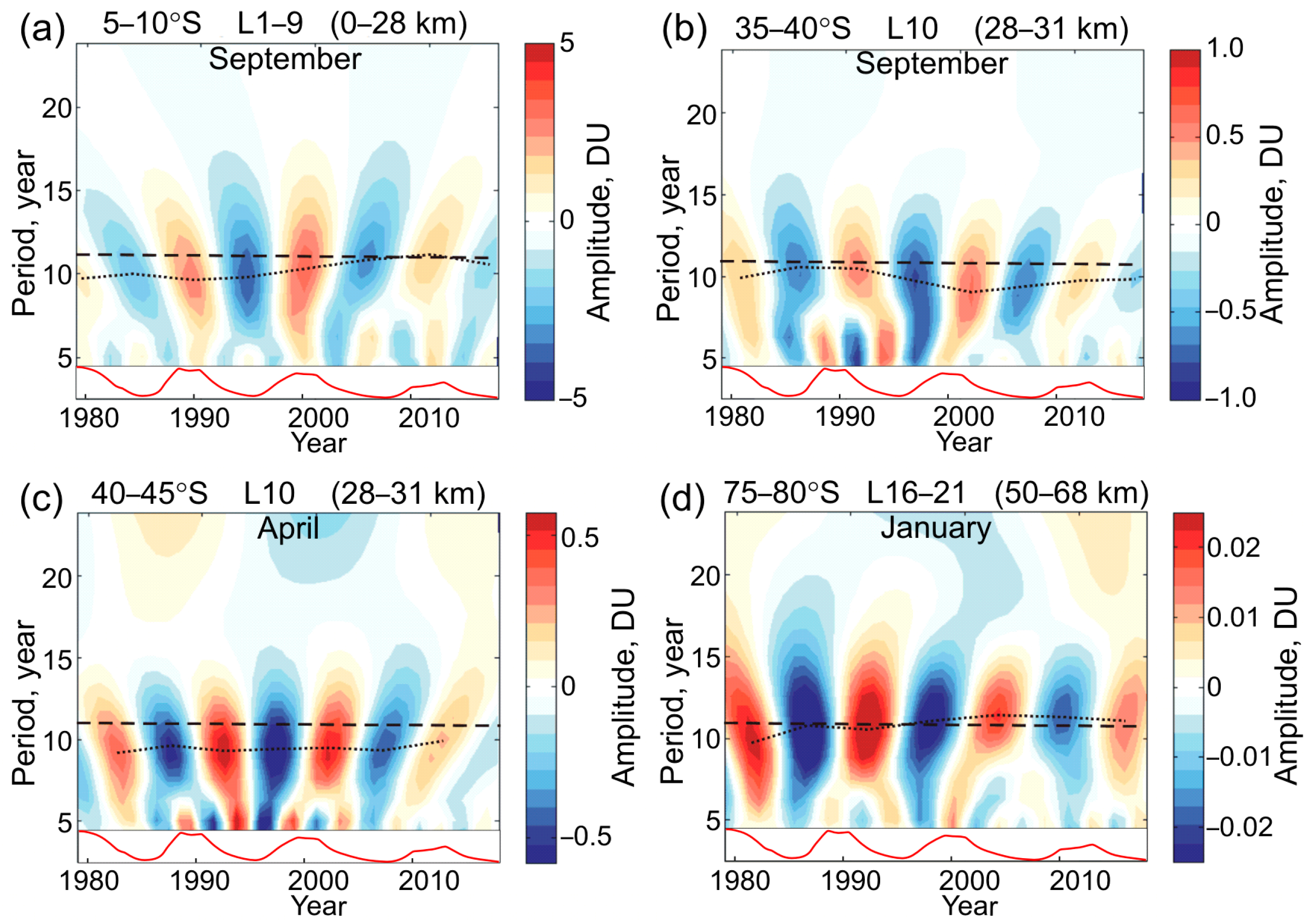
  • Lower SBUV layers L1–L9 in the tropics (0–28 km, Figure 8a);
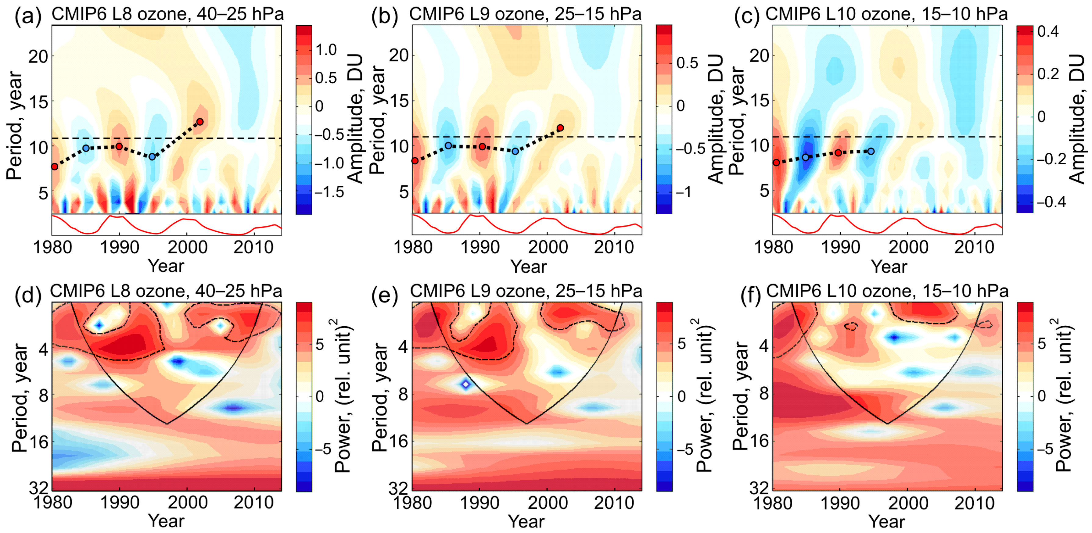
  • Lower–middle stratosphere in the SH extratropics, L9 and L10 (25–31 km, Figure 8b,c);
  • Middle–upper stratosphere in the tropics, L11–L15 (31–47 km, Figure 8d,e); and
  • Stratopause–lower mesosphere region, L16–L21, mostly in the SH (47–64 km, Figure 8f).
Because of the SBUV data gap in the high southern latitudes in austral winter, the seasonal changes in the solar activity–ozone response in the tropics and both hemispheres cannot be fully compared. Some conclusions can still be drawn. The strong solar signal concentrated in the tropics in L1–L9 (0–28 km) is obviously related to the lower stratosphere, since the tropospheric ozone amount (below the tropical tropopause, ~16 km) is small compared with the ozone amount at and around the stratospheric ozone maximum. As shown in many studies, the tropical lower-stratospheric response is produced mainly by a solar-induced modulation of the Brewer–Dobson circulation [33,39,76,77]. This mechanism suggests the solar-cycle-induced modulation of wave activity that impacts the BDC, as manifested by the weakening of the tropical upwelling that in turn would lead to adiabatic warming and higher ozone levels in the tropical lower stratosphere in solar maximum.
The strong tropical ozone response also forms the second maximum in the middle stratosphere in L11–L12 (31–37 km, Figure 8d). It is separated from the lower-stratospheric response maximum by the response minimum in L10 (28–31 km, Figure 8c). The altitudes of both the minimum and the two maxima in the tropical stratospheric ozone response to the solar cycle are generally consistent with recent studies that used the CMIP6 ozone database [26] and the artifact-corrected ozone composites [52]. It can be noted that the local Dobson record does not agree with CMIP6 (Figure 2b). The result of Figure 8d differs from the earlier estimates made by SBUV data by Soukharev and Hood [44], where the ozone response minimum was found at the L11–L12 altitudes. Possibly, this difference could be explained by the 15-year-shorter time series (1979–2003) used by Soukharev and Hood [44] and partly by the analysis method. In our work, the analysis of the relative intensity in the periodicities may be less sensitive to artifacts in datasets, which introduce uncertainties in the solar activity–ozone signal detection [52].
Outside the tropics, the most notable feature takes place in the lower and middle stratosphere with displacement of the solar cycle signal to the SH extratropics leading to the clear hemispheric asymmetry in L9–L10 (25–31 km, Figure 8b,c). Hemispheric asymmetry in the solar activity–ozone response was noted earlier [33,44,45]. In Figure 8b,c, the maximum solar signal in the high southern latitudes appears in autumn and spring. Hence, dynamical processes involved in the evolution of the winter polar vortex in the stratosphere seem to be of less importance. Similar asymmetry toward the SH stratosphere during austral autumn, winter, and spring exists also in the CMIP6 ozone database [26]. Unfortunately, the data gap in the SBUV layer ozone in winter prevents a full seasonal comparison. Confirmation of the latitude–season pattern in the solar signal shown here using independent analysis, including model verification, is required.
The hemispheric asymmetry in the solar activity–ozone response exists also in the mesosphere (Figure 8f). In the polar regions, the maximum responses are observed in the austral summer that indicate the radiative mechanism of the enhanced impact of the 11-year periodicity on the mesospheric ozone. The solar signal dominates also in the SH tropics and subtropics (Figure 8f); however, it maximizes in the cold seasons (austral autumn and winter, April–August). This implies possible solar modulation of an upwelling branch of the BDC and its hemispheric asymmetry. There are indications of similar hemispheric asymmetry in mesospheric ozone and its response to the solar cycle. Ozone profile data obtained from the Halogen Occultation Experiment (HALOE) during the period 1992–2004 show that the solar signal in the mesosphere in the mid-latitude zone 40–60° S is about three times stronger than in 40–60° N (see in Beig et al. [78], their Figure 6).
Ozone amounts and the amplitude of the 11-year variation of nighttime in upper mesosphere ozone from Microwave Limb Sounder (MLS) data increase toward the south pole in April–August and May–September [79], which is close to the maximum response timing in SH tropics and subtropics in Figure 8f. Due to the data gap, the SBUV layer ozone does not display if a similar anomaly exists in the winter polar region of the SH. Basing on the Sounding of the Atmosphere using Broadband Emission Radiometry (SABER) measurements in 2002–2016, Tang et al. [80] showed a strong asymmetry between the two hemispheres in the relationship between ozone density at the mesopause and solar activity. The ozone solar response is about twice as strong at the middle and high southern latitudes, although ozone density at the mesopause is symmetrical between the two hemispheres. Possible causes of this asymmetry need further clarification.
The most noticeable appearance of the quasi-11-year periodicity noted from Figure 8 is illustrated in Figure 9 using wavelet amplitude representation in year–period coordinates. Similar to the wavelets for Faraday/Vernadsky (Figure 5), the periodicity in zonal mean ozone is not as stable as in the 11-year solar cycle. The periods closest to 11 years (10–12 years) were revealed in the lowest layers L1–L9 in September (0–28 km, Figure 9a) and in the highest layers L16–L21 in January (47–64 km, Figure 9d) in the southern tropics and high latitudes, respectively.
In the middle stratosphere of the middle southern latitudes, the periods are systematically shorter (9–10 years, Figure 9b,c). As noted above in the case of Faraday/Vernadsky in the Antarctic Peninsula region (Figure 5), a difference in the mean periods leads to a phase shift of the ozone response relative to solar activity change.
The CMIP6 model data do not display a statistically significant signal near the 11-year period in the layers L8, L9, and L10 over Faraday/Vernadsky (Figure 10d–f), in which the SBUV data show a solar activity–ozone response at the 95% confidence level (Figure 7). Possibly, this is due to a weaker solar signal, since the wavelet amplitude in the CMIP6 layer ozone is a few times lower (Figure 10a–c) than that in SBUV (Figure 6). There are statistically significant short periods of 2–4 years in CMIP6 (Figure 10, bottom) and they show some similarity in timing to SBUV (Figure 7).

5. Conclusions

Ozone content in the terrestrial atmosphere is dependent on a series of chemical and dynamical factors, including ozone molecule production under solar ultraviolet radiation, their catalytic destruction under the influence of chlorine and bromine, variability due to large-scale atmospheric wave propagation, and Brewer–Dobson circulation. Dependence on solar ultraviolet radiation means that solar activity change can result in an ozone amount change. As discussed above, manifestations of the 11-year solar cycle were earlier identified in global ozone, in the lower and upper tropical stratosphere and in the mesosphere. In this paper, the vertical ozone distribution was investigated mainly using satellite SBUV instrument observations.
Ground-based Dobson spectrophotometer measurements and SBUV (V8.6) MOD overpass data for Faraday/Vernadsky station located in the Antarctic Peninsula region show almost identical interannual variations in total ozone, with a correlation coefficient r = 0.92 (1979–2018). Analysis shows that the solar cycle in total ozone over Faraday/Vernadsky is statistically insignificant in the wavelet power spectrum (Figure 5b,e). Nevertheless, from wavelet amplitude analysis, the quasi-11-year periodicity in total ozone shows qualitative consistency with the solar cycle in phase and in close correspondence with the mean relative amplitude (2.9%) to the global data. In the SBUV layer ozone, local response to the solar cycle is statistically significant at the 95% confidence level in the lower and middle stratosphere only (L8–L10, 22–31 km; Figure 7c–e).
The results show that the relative ozone changes between the solar minimum and maximum are 9.4%, 9.6%, and 6.8% in L8, L9, and L10, respectively. This is about 2–3 times larger than in the tropical stratosphere [26,52]. The strongest solar activity–ozone response is observed in the lower stratosphere at L8 and L9 (22–28 km), just above the climatological maximum in the vertical ozone profile. This is evidence of the dynamical factors, mainly affecting the stratospheric ozone at the high southern latitudes in response to the solar cycle. Since ozone in L8–L10 varies nearly in phase with the solar cycle (Figure 6c–e), anti-phase variations of the solar-induced anomalies in the Brewer–Dobson circulation (weakened meridional transport and high-latitude downwelling near the solar maximum) cannot be among the contributing factors. The process of the wave–mean flow interaction modulated by solar activity may be more important in terms of dynamically induced anomaly propagation from the upper stratosphere into the lower stratosphere contributing to ozone variations [76]. This possibility should be further investigated in models, considering the altitudinal, latitudinal, regional, and seasonal dependencies in the relationship between dynamical, chemical, and radiative effects.
Zonal mean SBUV ozone profiles show that the solar activity–ozone response is noticeably dependent on the latitude, altitude, and season, in agreement with many previous studies. The estimates of the solar signal in this work were made by calculating the ratio of the wavelet spectral power in the 10–12-year period range to the power in the studied period range of 2–33 years. This analysis method differs from that used in other works, where the relative change in the atmospheric variable between the solar minimum and maximum was estimated. The results indicate significant spatiotemporal anomalies in the manifestations of the solar cycle.
The strong solar activity–ozone response exists in the tropics in the lower SBUV layers L1–L9 (0–28 km, Figure 8a). This solar signal relates mainly to the lower tropical stratosphere, where there is a maximum in the vertical distribution of ozone. The second maximum in the solar signal is in the middle–upper tropical stratosphere in L11–L15 (31–47 km, Figure 8d,e). These altitudinal locations of the two maximum ozone responses in the tropical stratosphere agree with the artifact-corrected ozone composites of Ball et al. [52] and recent analyses using the CMIP6 ozone database [26], although we note that we did not see evidence of a significant solar cycle response in the CMIP6 data over Faraday/Vernadsky. It is assumed that the mechanism of solar-induced weakening of the Brewer–Dobson circulation near the solar cycle maximum is important for the tropical stratosphere ozone [39,76,77].
We also provided evidence of the stronger influence of the 11-year solar cycle on the atmosphere in the Southern Hemisphere relative to the Northern Hemisphere. The lower–middle stratosphere at L9 and L10 (25–31 km, Figure 8b,c) is characterized by strong hemispheric asymmetry with maximum (minimum) solar signal in the SH extratropics (in the tropics and the NH extratropics). On the whole, similar asymmetry toward the SH stratosphere during austral autumn, winter, and spring exists also in the CMIP6 ozone database [26]. However, additional analysis of the relevant mechanisms is needed in future studies.
The third maximum in the solar activity–ozone response in the tropics is in the stratopause–lower mesosphere region, L16–L21 (47–64 km, Figure 8f), and it extends mostly to the SH. Hemispheric asymmetry in the mesospheric ozone and its response to the solar cycle was noted in other works [78,79,80], although possible mechanisms need further clarification.

Author Contributions

Conceptualization, Y.Y.; methodology, A.G. and G.M.; software, A.G., Y.W. and O.I.; validation, A.G., O.E. and G.M.; investigation, O.E., A.G. and A.K.; writing—original draft preparation, A.G., O.E. and G.M.; writing—review and editing, A.G., O.E., A.K. and G.M.; visualization, O.E., A.G., Y.W. and O.I.; supervision, Y.Y. and A.K.; project administration, G.M. Each author contributed to the interpretation and discussion of the results and edited the manuscript. All authors have read and agreed to the published version of the manuscript.

Funding

This research received no external funding.

Acknowledgments

We acknowledge the Royal Observatory of Belgium SILSO World Data Center (http://www.sidc.be/silso/), the Natural Resources Canada (https://spaceweather.gc.ca/solarflux/sx-5-en.php) and LASP Interactive Solar Irradiance Datacenter (https://lasp.colorado.edu/lisird/data/penticton_radio_flux/) for free access to the monthly solar activity data. The authors also thank the team of the Goddard Space Flight Center NASA for free access to the SBUV Merged Ozone Data Set (MOD) 1970–2018 Profile and Total Column Ozone from the SBUV Instrument Series available at https://acd-ext.gsfc.nasa.gov/Data_services/merged/. We thank Goddard Earth Sciences Data and Information Services Center (GES DISC), Greenbelt, Maryland, USA, for MERRA-2 data, Copernicus Climate Change Service (https://cds.climate.copernicus.eu/cdsapp#!/home) for ERA-5 data and the WCRP Coupled Model Intercomparison Project (Phase 6) team for CMIP6 data. This work was partly supported by the Ministry of Education and Science of Ukraine through the projects 19BF051-08 and 20BF051-02 of the Taras Shevchenko National University of Kyiv, and by the National Academy of Sciences of Ukraine through the projects 0116U000035 and 0119U10180 of the Institute of Radio Astronomy, NAS of Ukraine. This work contributed to the National Antarctic Scientific Center of Ukraine research objectives, partly performed in College of Physics, International Center of Future Science of Jilin University, China, and contributed to Project 4293 of the Australian Antarctic Program.

Conflicts of Interest

The authors declare no conflict of interest.

References

  1. Rowland, F.S. Stratospheric Ozone Depletion. In Twenty Years of Ozone Decline, Proceedings of the Symposium for the 20th Anniversary of the Montreal Protocol; Zerefos, C., Contopoulos, G., Skalkeas, G., Eds.; Springer: Dodrecht, Germany, 2009; pp. 23–66. [Google Scholar] [CrossRef] [Green Version]
  2. Solomon, S.; Portmann, R.W.; Sasaki, T.; Hofmann, D.J.; Thompson, D.W.J. Four decades of ozonesonde measurements over Antarctica. J. Geophys. Res. 2005, 110, D21311. [Google Scholar] [CrossRef] [Green Version]
  3. Fabian, P.; Dameris, M. Ozone in the Atmosphere. Basic Principles, Natural and Human Impacts; Springer: Heidelberg, Germany, 2014; 137p. [Google Scholar] [CrossRef]
  4. Chipperfield, M.P.; Bekki, S.; Dhomse, S.; Harris, N.R.P.; Hassler, B.; Hossaini, R.; Steinbrecht, W.; Thieblemont, R.; Weber, M. Detecting recovery of the stratospheric ozone layer. Nature 2017, 549, 211–218. [Google Scholar] [CrossRef] [PubMed] [Green Version]
  5. Grytsai, A.V.; Evtushevsky, O.M.; Agapitov, O.V.; Klekociuk, A.R.; Milinevsky, G.P. Structure and long-term change in the zonal asymmetry in Antarctic total ozone during spring. Ann. Geophys. 2007, 25, 361–374. [Google Scholar] [CrossRef]
  6. Kuttippurath, J.; Nair, P.J. The signs of Antarctic ozone recovery. Sci. Rep. 2017, 7, 585. [Google Scholar] [CrossRef]
  7. Manney, G.; Santee, M.L.; Rex, M.; Livesey, N.J.; Pitts, M.C.; Veefkind, P.; Nash, E.R.; Wohltmann, I.; Lehmann, R.; Froidevaux, L.; et al. Unprecedented Arctic ozone loss in 2011. Nature 2011, 478, 469–477. [Google Scholar] [CrossRef]
  8. Pommereau, J.P.; Goutail, F.; Lefèvre, F.; Pazmino, A.; Adams, C.; Dorokhov, V.; Eriksen, P.; Kivi, R.; Stebel, K.; Zhao, X.; et al. Why unprecedented ozone loss in the Arctic in 2011? Is it related to climate change? Atmos. Chem. Phys. 2013, 13, 5299–5308. [Google Scholar] [CrossRef] [Green Version]
  9. Witze, A. Rare ozone hole opens over Arctic—and it’s big. Nature 2020, 580, 18–19. [Google Scholar] [CrossRef] [Green Version]
  10. 2020/2021 Arctic OMPS and MERRA-2 Ozone. Available online: https://ozonewatch.gsfc.nasa.gov/meteorology/NH.html (accessed on 24 July 2020).
  11. Solomon, S.; Ivy, D.J.; Kinnison, D.; Mills, M.J.; Neely, R.R.; Schmidt, A. Emergence of healing in the Antarctic ozone layer. Science 2016, 353, 269–274. [Google Scholar] [CrossRef] [Green Version]
  12. Tegtmeier, S.; Fioletov, V.E.; Shepherd, T.G. Seasonal persistence of northern low- and middle-latitude anomalies of ozone and other trace gases in the upper stratosphere. J. Geophys. Res. 2008, 113, D21308. [Google Scholar] [CrossRef]
  13. Randall, C.E.; Harvey, V.L.; Singleton, C.S.; Bernath, P.F.; Boone, C.D.; Kozyra, J.U. Enhanced NOx in 2006 linked to strong upper stratospheric Arctic vortex. Geophys. Res. Lett. 2006, 33, L18811. [Google Scholar] [CrossRef]
  14. Kuchar, A.; Sacha, P.; Miksovsky, J.; Pisoft, P. The 11-year solar cycle in current reanalyses: A (non)linear attribution study of the middle atmosphere. Atmos. Chem. Phys. 2015, 15, 6879–6895. [Google Scholar] [CrossRef] [Green Version]
  15. Shepherd, T.G.; McLandress, C. A robust mechanism for strengthening of the Brewer–Dobson circulation in response to climate change: Critical-layer control of Subtropical wave breaking. J. Atmos. Sci. 2011, 68, 784–797. [Google Scholar] [CrossRef]
  16. Kim, J.Y.; Chun, H.Y.; Kang, M.J. Changes in the Brewer-Dobson circulation for 1980-2009 revealed in MERRA reanalysis data. Asia Pac. J. Atmos. Sci. 2014, 50, 73–92. [Google Scholar] [CrossRef]
  17. Shepherd, T.G. Large-scale atmospheric dynamics for atmospheric chemists. Chem. Rev. 2003, 103, 4509–4532. [Google Scholar] [CrossRef]
  18. Tegtmeier, S.; Fioletov, V.E.; Shepherd, T.G. A global picture of the seasonal persistence of stratospheric ozone anomalies. J. Geophys. Res. 2010, 115, D18119. [Google Scholar] [CrossRef]
  19. Bekki, S.; Lefevre, F. Stratospheric ozone: History and concepts and interactions with climate. Eur. Phys. J. Conf. 2009, 1, 113–136. [Google Scholar] [CrossRef] [Green Version]
  20. Lean, J.L.; Rottman, G.J.; Kyle, H.L.; Woods, T.N.; Hickey, J.R.; Puga, L.C. Detection and parameterization of variations in solar mid- and near-ultraviolet radiation (200–400 nm). J. Geophys. Res. 1997, 102, 29939–29956. [Google Scholar] [CrossRef]
  21. Rottman, G.; Woods, T.; Snow, M.; DeToma, G. The solar cycle variation in ultraviolet irradiance. Adv. Space Res. 2001, 27, 1927–1932. [Google Scholar] [CrossRef]
  22. Lean, J.L.; DeLand, M.T. How does the Sun’s spectrum vary? J. Clim. 2012, 25, 2555–2560. [Google Scholar] [CrossRef]
  23. Hathaway, D.H. The solar cycle. Living Rev. Sol. Phys. 2015, 12, 4. [Google Scholar] [CrossRef]
  24. Covington, A.E. Solar radio emission at 10.7 cm, 1947–1968. J. R. Astron. Soc. Can. 1969, 63, 125–132. Available online: http://adsabs.harvard.edu/full/1969JRASC..63..125C (accessed on 23 July 2020).
  25. Tapping, K.F. Recent solar radio astronomy at centimeter wavelengths: The variability of the 10.7-cm flux. J. Geophys. Res. 1987, 92, 829–838. [Google Scholar] [CrossRef]
  26. Maycock, A.C.; Matthes, K.; Tegtmeier, S.; Schmidt, H.; Thiéblemont, R.; Hood, L.; Akiyoshi, H.; Bekki, S.; Deushi, M.; Jöckel, P.; et al. The representation of solar cycle signals in stratospheric ozone—Part 2: Analysis of global models. Atmos. Chem. Phys. 2018, 18, 11323–11343. [Google Scholar] [CrossRef] [Green Version]
  27. Khrgian, A.K.; Kuznetsov, G.I.; Kondrat’eva, A.V. Atmospheric Ozone; Translated from Russian; Jerusalem (Israel Program for Scientific Translations) Humphrey: London, UK, 1969; 90p. [Google Scholar]
  28. Zerefos, C.S.; Crutzen, P.J. Stratospheric thickness variations over the northern hemisphere and their possible relation to solar activity. J. Geophys. Res. 1975, 80, 5041–5043. [Google Scholar] [CrossRef]
  29. Keating, G.M. The response of ozone to solar activity variations: A review. Sol. Phys. 1981, 74, 321–347. [Google Scholar] [CrossRef]
  30. Zerefos, C.S.; Tourpali, K.; Bojkov, B.; Balis, D.S.; Rognerund, B.; Isaksen, I.S.A. Solar activity–total column ozone relationships: Observations and model studies with heterogeneous chemistry. J. Geophys. Res. 1997, 102, 1561–1570. [Google Scholar] [CrossRef]
  31. Bisht, H.; Pande, B.; Chandra, R.; Pande, S. Statistical study of different solar activity features with total column ozone at two hill stations of Uttarakhand. Indian J. Radio Space Phys. 2014, 43, 251–262. Available online: https://shodhganga.inflibnet.ac.in/bitstream/10603/215321/18/zrsp-886-paper%201.pdf (accessed on 23 July 2020).
  32. González-Navarrete, J.C.; Salamanca, J.; Pinzón-Verano, I.M. Ozone layer adaptive model from direct relationship between solar activity and total column ozone for the tropical equator-Andes-Colombian region. Atmósfera 2018, 31, 155–164. [Google Scholar] [CrossRef] [Green Version]
  33. Hood, L.L. The solar cycle variation of total ozone: Dynamical forcing in the lower stratosphere. J. Geophys. Res. 1997, 102, 1355–1370. [Google Scholar] [CrossRef] [Green Version]
  34. Fioletov, V.E.; Shepherd, T.G. Seasonal persistence of midlatitude total ozone anomalies. Geophys. Res. Lett. 2003, 30, 1417. [Google Scholar] [CrossRef] [Green Version]
  35. Thiéblemont, R.; Marchand, M.; Bekki, S.; Bossay, S.; Lefèvre, F.; Meftah, M.; Hauchecorne, A. Sensitivity of the tropical stratospheric ozone response to the solar rotational cycle in observations and chemistry–climate model simulations. Atmos. Chem. Phys. 2017, 17, 9897–9916. [Google Scholar] [CrossRef] [Green Version]
  36. Zerefos, C.S.; Tourpali, K.; Balis, D. Solar activity–ozone relationships in the vertical distribution of ozone. Int. J. Remote Sens. 2005, 26, 3449–3454. [Google Scholar] [CrossRef]
  37. Isaksen, I.S.A.; Rognerud, B.; Myhre, G.; Haigh, J.D.; Rumbold, S.T.; Shine, K.P.; Zerefos, C.; Tourpali, K.; Randel, W. Radiative forcing from modelled and observed stratospheric ozone changes due to the 11-year solar cycle. Atmos. Chem. Phys. Discuss. 2008, 8, 4353–4371. [Google Scholar] [CrossRef] [Green Version]
  38. Calisesi, Y.; Matthes, K. The middle atmospheric ozone response to the 11-year solar cycle. Space Sci. Rev. 2006, 125, 273–286. [Google Scholar] [CrossRef]
  39. Hood, L.L.; Soukharev, B.E. The lower-stratospheric response to 11-yr solar forcing: Coupling to the troposphere–ocean response. J. Atmos. Sci. 2012, 69, 1841–1864. [Google Scholar] [CrossRef] [Green Version]
  40. Bordi, I.; Berrilli, F.; Pietropaolo, E. Long-term response of stratospheric ozone and temperature to solar variability. Ann. Geophys. 2015, 33, 267–277. [Google Scholar] [CrossRef] [Green Version]
  41. Gruzdev, A.N. Estimate of the effect of the 11-year solar activity cycle on the ozone content in the stratosphere. Geomag. Aeron. 2014, 54, 633–639. [Google Scholar] [CrossRef]
  42. Maycock, A.C.; Matthes, K.; Tegtmeier, S.; Thiéblemont, R.; Hood, L. The representation of solar cycle signals in stratospheric ozone—Part 1: A comparison of recently updated satellite observations. Atmos. Chem. Phys. 2016, 16, 10021–10043. [Google Scholar] [CrossRef] [Green Version]
  43. Dhomse, S.S.; Chipperfield, M.P.; Damadeo, R.P.; Zawodny, J.M.; Ball, W.T.; Feng, W.; Hossaini, R.; Mann, G.W.; Haigh, J.D. On the ambiguous nature of the 11 year solar cycle signal in upper stratospheric ozone. Geophys. Res. Lett. 2016, 43, 7241–7249. [Google Scholar] [CrossRef]
  44. Soukharev, B.E.; Hood, L.L. Solar cycle variation of stratospheric ozone: Multiple regression analysis of long-term satellite data sets and comparisons with models. J. Geophys. Res. 2006, 111, D20314. [Google Scholar] [CrossRef] [Green Version]
  45. Tourpali, K.; Zerefos, C.S.; Balis, D.S.; Bais, A.F. The 11-year solar cycle in stratospheric ozone: Comparison between Umkehr and SBUVv8 and effects on surface erythemal irradiance. J. Geophys. Res. 2007, 112, D12306. [Google Scholar] [CrossRef]
  46. Langematz, U.; Tully, M.; Calvo, N.; Dameris, M.; de Laat, A.T.J.; Klekociuk, A.; Müller, R.; Young, P. Polar stratospheric ozone: Past, Present, and Future. In Chapter 4 in Scientific Assessment of Ozone Depletion: 2018; Global Ozone Research and Monitoring Project—Report No. 58; World Meteorological Organization: Geneva, Switzerland, 2018; pp. 4.1–4.63. Available online: https://www.esrl.noaa.gov/csl/assessments/ozone/2018/ (accessed on 23 July 2020).
  47. Dameris, M.; Matthes, S.; Deckert, R.; Grewe, V.; Ponater, M. Solar cycle effect delays onset of ozone recovery. Geophys. Res. Lett. 2006, 33, L03806. [Google Scholar] [CrossRef]
  48. Arsenovic, P.; Rozanov, E.; Anet, J.; Stenke, A.; Schmutz, W.; Peter, T. Implications of potential future grand solar minimum for ozone layer and climate. Atmos. Chem. Phys. 2018, 18, 3469–3483. [Google Scholar] [CrossRef] [Green Version]
  49. Haigh, J.D. The Sun and the Earth’s climate. Living Rev. Sol. Phys. 2007, 4, 2. [Google Scholar] [CrossRef] [Green Version]
  50. Gray, L.J.; Beer, J.; Geller, M.; Haigh, J.D.; Lockwood, M.; Matthes, K.; Cubasch, U.; Fleitmann, D.; Harrison, G.; Hood, L.; et al. Solar influences on climate. Rev. Geophys. 2010, 48, RG4001. [Google Scholar] [CrossRef]
  51. Braesicke, P.; Neu, J.; Fioletov, V.; Godin-Beekmann, S.; Hubert, D.; Petropavlovskikh, I.; Shiotani, M.; Sinnhuber, B.M. Update on Global Ozone: Past, Present, and Future. In Chapter 3 in Scientific Assessment of Ozone Depletion: 2018; Global Ozone Research and Monitoring Project—Report No. 58; World Meteorological Organization: Geneva, Switzerland, 2019; pp. 3.1–3.74. Available online: https://www.esrl.noaa.gov/csl/assessments/ozone/2018/ (accessed on 23 July 2020).
  52. Ball, W.T.; Rozanov, E.; Alsing, J.A.; Marsh, D.R.; Tummon, F.; Mortlock, D.J.; Kinnison, D.; Haigh, J.D. The upper stratospheric solar cycle ozone response. Geophys. Res. Lett. 2019, 46, 1831–1841. [Google Scholar] [CrossRef] [Green Version]
  53. Hassler, B.; Bodeker, G.E.; Solomon, S.; Young, P.J. Changes in the polar vortex: Effects on Antarctic total ozone observations at various stations. Geophys. Res. Lett. 2011, 38, L01805. [Google Scholar] [CrossRef] [Green Version]
  54. Grytsai, A.; Klekociuk, A.; Milinevsky, G.; Evtushevsky, O.; Stone, K. Evolution of the eastward shift in the quasi-stationary minimum of the Antarctic total ozone column. Atmos. Chem. Phys. 2017, 17, 1741–1758. [Google Scholar] [CrossRef] [Green Version]
  55. Monthly Mean Ozone from OMI. Available online: http://www.temis.nl/protocols/o3field/o3mean_omi.php (accessed on 23 July 2020).
  56. Frith, S.M.; Kramarova, N.A.; Stolarski, R.S.; McPeters, R.D.; Bhartia, P.K.; Labow, G.J. Recent changes in total column ozone based on the SBUV Version 8.6 Merged Ozone Data Set. J. Geophys. Res. Atmos. 2014, 119, 9735–9751. [Google Scholar] [CrossRef]
  57. SBUV Merged Ozone Data Set (MOD), 1970-2018 Profile and Total Column Ozone from the SBUV Instrument Series. Available online: https://acd-ext.gsfc.nasa.gov/Data_services/merged/ (accessed on 23 July 2020).
  58. SBUV (Version 8.6) Instrument Summary, Daily Overpass Profiles at Specified Stations. Available online: https://acd-ext.gsfc.nasa.gov/anonftp/toms/sbuv/AGGREGATED/ (accessed on 23 July 2020).
  59. Komhyr, W.D.; Evans, R.D. Operations Handbook—Ozone Observations with a Dobson Spectrophotometer; World Meteorological Organization Global Ozone Research and Monitoring Project; NOAA/ESRL Global Monitoring Division: Geneva, Switzerland, 2006; 91p, Available online: https://library.wmo.int/doc_num.php?explnum_id=9405 (accessed on 23 July 2020).
  60. Grytsai, A.V.; Milinevsky, G.P.; Ivaniga, O.I. Total ozone over Vernadsky Antarctic station: Ground-based and satellite measurements. Ukr. Antarct. J. 2018, 17, 65–72. [Google Scholar] [CrossRef] [Green Version]
  61. ERA5 Monthly Averaged Data on Single Levels from 1979 to Present. Available online: https://cds.climate.copernicus.eu/cdsapp#!/dataset/reanalysis-era5-single-levels-monthly-means?tab=overview (accessed on 27 July 2020).
  62. Hersbach, H.; Bell, B.; Berrisford, P.; Hirahara, S.; Horányi, A.; Muñoz-Sabater, J.; Nicolas, J.; Peubey, C.; Radu, R.; Schepers, D.; et al. The ERA5 global reanalysis. Q. J. R. Meteor. Soc. 2020, 1–51. [Google Scholar] [CrossRef]
  63. M2TMNXSLV: MERRA-2 tavgM_2d_slv_Nx: 2d, Monthly Mean, Time-Averaged, Single-Level, Assimilation, Single-Level Diagnostics V5.12.4. Available online: https://disc.gsfc.nasa.gov/datasets/M2TMNXSLV_5.12.4/summary (accessed on 27 July 2020).
  64. Wargan, K.; Labow, G.; Frith, S.; Pawson, S.; Livesey, N.; Partyka, G. Evaluation of the ozone fields in NASA’s MERRA-2 reanalysis. J. Clim. 2017, 30, 2961–2988. [Google Scholar] [CrossRef] [PubMed] [Green Version]
  65. WCRP Coupled Model Intercomparison Project (Phase 6). Available online: https://esgf-node.llnl.gov/projects/cmip6/ (accessed on 27 July 2020).
  66. Checa-Garcia, R.; Hegglin, M.I.; Kinnison, D.; Plummer, D.A.; Shine, K.P. Historical tropospheric and stratospheric ozone radiative forcing using the CMIP6 database. Geophys. Res. Lett. 2018, 45, 3264–3273. [Google Scholar] [CrossRef] [Green Version]
  67. Kramarova, N.A.; Frith, S.M.; Bhartia, P.K.; McPeters, R.D.; Taylor, S.L.; Fisher, B.L.; Labow, G.J.; DeLand, M.T. Validation of ozone monthly zonal mean profiles obtained from the version 8.6 Solar Backscatter Ultraviolet algorithm. Atmos. Chem. Phys. 2013, 13, 6887–6905. [Google Scholar] [CrossRef] [Green Version]
  68. Chiou, E.W.; Bhartia, P.K.; McPeters, R.D.; Loyola, D.G.; Coldewey-Egbers, M.; Fioletov, V.E.; Van Roozendael, M.; Spurr, R.; Lerot, C.; Frith, S.M. Comparison of profile total ozone from SBUV (v8.6) with GOME-type and ground-based total ozone for a 16-year period (1996 to 2011). Atmos. Meas. Tech. 2014, 7, 1681–1692. [Google Scholar] [CrossRef] [Green Version]
  69. Sunspot Index and Long-term Solar Observations. Available online: http://www.sidc.be/silso/DATA/SN_m_tot_V2.0.txt (accessed on 23 July 2020).
  70. Natural Resources Canada, Space Weather Canada, Solar Radio Flux–Archive of Measurements. Available online: https://spaceweather.gc.ca/solarflux/sx-5-en.php (accessed on 20 July 2020).
  71. Lasp Interactive Solar Irradiance Datacenter, Penticton Solar Radio Flux at 10.7cm, Time Series. Available online: https://lasp.colorado.edu/lisird/data/penticton_radio_flux/ (accessed on 23 July 2020).
  72. Torrence, C.; Compo, G.P. A practical guide to wavelet analysis. Bull. Am. Meteorol. Soc. 1998, 79, 61–78. [Google Scholar] [CrossRef] [Green Version]
  73. Lean, J.; Rind, D. Climate forcing by changing solar radiation. J. Clim. 1998, 11, 3069–3094. [Google Scholar] [CrossRef]
  74. Angell, J.K. On the relation between atmospheric ozone and sunspot number. J. Clim. 1989, 2, 1404–1416. [Google Scholar] [CrossRef] [Green Version]
  75. Efstathiou, M.N.; Varotsos, C.A. On the 11 year solar cycle signature in global total ozone dynamics. Meteorol. Appl. 2013, 20, 72–79. [Google Scholar] [CrossRef]
  76. Kodera, K.; Kuroda, Y. Dynamical response to the solar cycle. J. Geophys. Res. 2002, 107, 4749. [Google Scholar] [CrossRef] [Green Version]
  77. Bednarz, E.M.; Maycock, A.C.; Telford, P.J.; Braesicke, P.; Abraham, N.L.; Pyle, J.A. Simulating the atmospheric response to the 11-year solar cycle forcing with the UM-UKCA model: The role of detection method and natural variability. Atmos. Chem. Phys. 2019, 19, 5209–5233. [Google Scholar] [CrossRef] [Green Version]
  78. Beig, G.; Fadnavis, S.; Schmidt, H.; Brasseur, G.P. Inter-comparison of 11-year solar cycle response in mesospheric ozone and temperature obtained by HALOE satellite data and HAMMONIA model. J. Geophys. Res. 2012, 117, D00P10. [Google Scholar] [CrossRef]
  79. Lee, J.N.; Wu, D.L. Solar cycle modulation of nighttime ozone near the mesopause as observed by MLS. Earth Space Sci. 2020, 6, e2019EA001063. [Google Scholar] [CrossRef]
  80. Tang, C.; Wu, B.; Wei, Y.; Qing, C.; Dai, C.; Li, J.; Wei, H. The responses of ozone density to solar activity in the mesopause region and the mutual relationship based on SABER measurements during 2002–2016. J. Geophys. Res. Space Phys. 2018, 123, 3039–3049. [Google Scholar] [CrossRef]
Figure 1. Total ozone monthly mean in October 2018 over southern polar region. White contour outlines the ozone hole edge at the 220-DU total ozone level. The Antarctic station Faraday/Vernadsky is shown by the white circle, modified from [55].
Atmosphere 11 00873 g001
Figure 2. (a) The 40-year annual mean climatology (1979–2018) of the SBUV layer ozone column over Faraday/Vernadsky. SBUV layer numbers 1–16 between the pressure levels 1013 and 1 hPa (0–50 km) are indicated. Standard deviations are shown by horizontal bars. Data from [58] are presented. (b) Time series of annual mean Dobson spectrophotometer (red), the Solar Backscatter Ultra Violet (SBUV) radiometer (yellow), the Coupled Model Intercomparison Project Phase 6 (CMIP6) (green), the European Centre for Medium-Range Weather Forecasts 5th (ERA5) reanalysis (blue), and the Modern-Era Retrospective analysis for Research and Applications Version 2 (MERRA2) reanalysis (black) total ozone over Faraday/Vernadsky, 1979–2019, except for CMIP6 for 1980–2014 and SBUV for 1979–2018 [58,61,63,65].
Atmosphere 11 00873 g002
Figure 3. The sunspot numbers (red curve) and the 10.7 cm solar flux (F10.7, blue curve) from the middle of the 20th century [69,70,71]. The F10.7 values are in solar flux units (sfu), 1 sfu is equal to 10–22 W m–2·Hz–1. The observed F10.7 is presented on the right axis.
Atmosphere 11 00873 g003
Figure 4. (a) The wavelet transform with the real part of the Morlet function for sunspot number time series in 1947–2018; red (blue) shows the location of the maxima (minima) of the solar cycle signal in the coordinates ‘year–period’; solid line marks a period of 11 years and a black dashed curve is drawn through the peak intensities of the wavelet transform. (b) Power spectrum of the wavelet transform shown in (a) and the solid curve is the cone of influence, within which the spectrum is not significantly influenced by boundary effects. (c) Global wavelet spectrum for (b). Contour in (b) and dashed curve in (c) show the 95% confidence level with the red-noise background spectrum calculated for a lag-1 autocorrelation of 0.7. The cone of influence is shown as a lighter shade. Wavelet transform with the mother wavelet ψ ( t ) = e t 2 / 2 · e i · 6 t is used. Dashed horizontal lines in (c) mark the peak power in the global wavelet spectrum between the periods of 10 and 12 years. Note the difference in scale for periods in (b) and (c) from (a).
Atmosphere 11 00873 g004
Figure 5. As in Figure 4, but for total ozone over Faraday/Vernadsky in 1979–2018 from (ac) Dobson spectrophotometer measurements and (df) SBUV data. Red curve at the bottom in (a) and (d) is the smoothed time series of the sunspot number from Figure 3 (red curve).
Atmosphere 11 00873 g005
Figure 6. As in Figure 5a,d, but for SBUV layer ozone over Faraday/Vernadsky at (a) 0–3 km altitudes (L1) and (bf) 19–34 km (L7–L11; see Figure 2).
Atmosphere 11 00873 g006
Figure 7. Periodicity in ozone variations over Faraday/Vernadsky from wavelet power spectra for the same layers L1 and L7–L11 as in Figure 6. From SBUV layer ozone data over Faraday/Vernadsky at (a) 0–3 km altitudes (L1) and (bf) 19–34 km (L7–L11; see Figure 2). Contours show the 95% confidence level with lag-1 autocorrelation of 0.7.
Atmosphere 11 00873 g007
Figure 8. Ratio of the intensity of the wavelet transform with periods of 10–12 years to the intensity of periods of 2–33 years in (a) L1–L8 poleward of 20° latitude and L1–L9 equatorward of 20° latitude marked by dashed lines and signed arrows, (b) L9 poleward of 20° latitude, (c) L10, (d) L11–L12, (e) L13–L15, and (f) L16–L21. Contours show the 95% confidence level. Note the different color scale in Figure 8f due to lower ratios.
Atmosphere 11 00873 g008
Figure 9. The most prominent quasi-11-year periods in the zonal mean SBUV MOD data at latitudes (a) 5–10° S, L1–9 and (b) 35–40° S, L10, in September; (c) 40–45° S, L10 in April and (d) 75–80° S, L16–21 in January.
Atmosphere 11 00873 g009
Figure 10. (ac) Wavelet amplitude and (df) wavelet power spectrum for CMIP6 ozone over Faraday/Vernadsky in the layers (a,d) L8, (b,e) L9, and (c,f) L10, where SBUV data show statistically significant quasi-11-year periodicity.
Atmosphere 11 00873 g010
Table 1. Pearson’s linear correlation coefficient between annual mean total ozone over Faraday/Vernadsky measured with the Dobson spectrophotometer and retrieved from the Solar Backscatter Ultra Violet (SBUV) radiometer, the European Centre for Medium-Range Weather Forecasts 5th (ERA5) reanalysis, the Modern-Era Retrospective analysis for Research and Applications Version 2 (MERRA2) reanalysis, and the Coupled Model Intercomparison Project Phase 6 (CMIP6) data.
DataSBUVERA5MERRA2CMIP6
Dobson0.920.840.860.51
SBUV 0.900.910.60
ERA5 0.920.69
MERRA2 0.69

