Article

Investigating the Interannual Variability of the Boreal Summer Water Vapor Source and Sink over the Tropical Eastern Indian Ocean-Western Pacific

1
School of Atmospheric Sciences, Sun Yat-sen University, Zhuhai 519082, China
2
Key Laboratory of Tropical Atmosphere-Ocean System (Sun Yat-sen University), Ministry of Education, Zhuhai 519082, China
3
Southern Marine Science and Engineering Guangdong Laboratory, Zhuhai 519082, China
4
School of Physical Science and Technology, Yangzhou University, Yangzhou 225000, China
5
Laboratory for Climate Studies, National Climate Center, China Meteorological Administration, Beijing 100081, China
*
Author to whom correspondence should be addressed.
Atmosphere 2020, 11(7), 758; https://doi.org/10.3390/atmos11070758
Submission received: 8 June 2020 / Revised: 2 July 2020 / Accepted: 14 July 2020 / Published: 17 July 2020
(This article belongs to the Section Meteorology)

Abstract

:
Using the four-times daily and monthly-mean reanalysis datasets of NCEP/NCAR for the 1958 to 2018 period, we investigate the interannual variability of the June-July-August (JJA)–mean water vapor source and sink over the tropical eastern Indian Ocean-Western Pacific (TEIOWP) and the underlying mechanism. It is found that the two major modes (EOF1 and EOF2) of the water vapor source and sink anomalies over the TEIOWP present a southwest-northeast oriented dipole and a southwest-northeast oriented tripole. Specifically, when the western maritime continent shows an anomalous water vapor source, the northwestern Pacific is characterized by anomalous water vapor sink and source in EOF1 and EOF2 modes, respectively. The EOF1 and EOF2 modes are primarily driven by a single and a double meridional cell anomaly, which corresponds to the in-phase and out-of-phase linkage between evaporation anomalies over the western maritime continent and precipitation anomalies over the northwestern Pacific, respectively. Furthermore, the EOF1 mode is regulated by the quick transition of the El Niño-Southern Oscillation (ENSO) phase, whereas the EOF2 mode probably originates from internal atmospheric variability. Considering that the standard deviation of PC1 is much higher during ENSO years than that during non-ENSO years, it is probable that the water source and sink anomalies over the TEIOWP tend to be dominant by EOF1 mode during ENSO years. In contrast, the EOF2 mode may play an important role in the water source and sink anomalies over the TEIOWP during non-ENSO years. Accordingly, the water vapor source and sink anomalies over the TEIOWP may be well predicted based on the ENSO state in the previous December-January-February. These results are useful for understanding the predictability of water vapor source and sink anomalies over the TEIOWP.

1. Introduction

Although the water vapor in the atmosphere accounts for only 0.001% of the global water, this tiny fraction is the most active part of the water cycle [1,2]. The atmospheric water cycle mainly includes evaporation, water vapor transport and precipitation, linking water exchange among ocean, land and different regions. The water vapor is mostly concentrated in the lower atmosphere and decreases rapidly with the increase of altitude. Meanwhile, the water vapor over the equator is abundant and it decreases significantly towards the North and South poles. As the central part of the warm pool, the tropical eastern Indian Ocean-western Pacific (TEIOWP) is the most abundant region of water vapor in the world [2,3].
East Asia is situated to the west of the Pacific and to the east of the Tibet Plateau, where the atmospheric circulation has a distinct seasonal variation and shows a distinct monsoon climate. In June-July-August (JJA), the East Asian summer monsoon (EASM) carries abundant water vapor from the ocean to the land. The advance and retreat of EASM correspond to the change of water vapor transport intensity, which results in the northward and southward movement of the JJA precipitation belt over East Asia [4]. The water vapor transport over East Asia in JJA mainly includes three water vapor inflows: (1) the southwestward water vapor from the Indian Ocean to Eastern China through the Bay of Bengal, Indo-China Peninsula and South China Sea; (2) the southeastward water vapor from the western Pacific to eastern China along the southwestern margin of the western Pacific subtropical high (WPSH); (3) zonal water vapor transport along the westerlies belt over the middle latitudes [4]. Among them, the water vapor from the TEIOWP plays a dominant role in JJA precipitation anomalies over East Asia [4].
The sea surface temperature (SST) over the tropical Pacific and tropical Indian Ocean are considered to be important external forcings affecting the interannual variability of water vapor over the TEIOWP and the EASM [5,6,7]. First, the El Niño-Southern Oscillation (ENSO) has a great impact on precipitation anomalies over East Asia, and this influence depends on the stages of the ENSO [8,9,10]. During the JJA in the El Niño developing phase, both the WPSH and the water vapor transport from the TEIOWP are weakened, favoring dry anomalies over Central-North China [11]. During the JJA in the El Niño decaying phase, an anomalous anticyclone appeared over the northwestern Pacific, which corresponds to an enhanced WPSH and increases the precipitation in the middle and lower reaches of the Yangtze River [8,9,12].
Both the Indian Ocean Basin-Wide (IOBW) mode and tropical Indian Ocean dipole (TIOD) mode are important factors regulating the interannual variability of the EASM. The IOBW plays an important “charger” role in ENSO decaying summers, which tends to increase (decrease) the precipitation over the middle and lower reaches of the Yangtze River in its positive (negative) phase [13,14,15]. The TIOD is featured by obvious seasonal differences, and it usually begins in the May-June, reaches the peak in September-October-November (SON), and rapidly decays in December-January-February (DJF). When the TIOD displays a positive (negative) phase in JJA, the southwestward water vapor from the Indian Ocean to Eastern China is increased (decreased), which contributes to more (less) than normal precipitation over South China [16]. Overall, the water vapor anomalies over the TEIOWP is crucial in linking the external forcings and JJA precipitation anomalies over East Asia.
In JJA, the water vapor source and sink are mainly located in the Southern Hemisphere and Northern Hemisphere, respectively [3,17,18]. Correspondingly, water vapor that is lost in the Southern Hemisphere is transported to the Indian and East Asian monsoon regions by cross-equatorial flows. Variations in the water vapor source and sink over the TEIOWP effectively impact the JJA precipitation anomalies over East Asia [19,20]. For instance, Zhou and Yu [19] found that positive precipitation anomalies over the middle and lower reaches of the Yangtze River are related to anomalous water vapor from the Philippine Sea and the Bay of Bengal. While the anomalous water vapor from the northwestern Pacific contributes to the increased precipitation over the Huaihe River valley. For a more complete understanding of the interannual variations of the water vapor over the TEIOWP, we need to address two questions: what are the major modes of the water vapor source and sink anomalies over the TEIOWP? What are the possible linkages between the major modes and the external forcings? To address the above questions, we will first analyze the characteristics of the two major modes of anomalous water vapor source and sink over the TEIOWP. Then, we will investigate the mechanism responsible for the two major modes. Specifically, we will identify the contribution of the ENSO and TIOD to the two major modes of the water vapor source and sink anomalies over the TEIOWP.
The rest of the article is organized as follows. The data and methods employed are described in Section 2. Section 3 presents the characteristics of the two major modes of anomalous water vapor source and sink over the TEIOWP. Section 4 investigates the possible impact of the external forcings on water vapor source and sink anomalies over the TEIOWP. A summary along with a discussion is given in Section 5 and Section 6, respectively.

2. Data and Method

2.1. Datasets

The National Center for Environmental Prediction (NCEP)/National Center for Atmospheric Research (NCAR) reanalysis data, including the four-times daily zonal, meridional and vertical wind components, relative humidity, and monthly mean meridional and vertical wind components were employed to analyze water vapor source and sink and large-scale atmospheric circulation anomalies, and they are available from 1948 to the present [21]. These variables have a horizontal resolution of 2.5° × 2.5°, except for the 10-m wind, which are on T62 Gaussian grids. The monthly mean Niño3.4 index was downloaded from the Climate Prediction Center (CPC) website [22]. The monthly mean SST data used in the present study is the Extended Reconstructed SST version 5 (ERSST5) dataset, which was provided by the National Oceanic and Atmospheric Administration (NOAA)/Oceanic and Atmospheric Research (OAR)/Earth System Research Laboratory Physical Science Division (ERSL PSD). This dataset has a horizontal resolution of 2.0° × 2.0° and is available from 1854 to the present [23]. The monthly precipitations were derived from the NOAA global monthly precipitation reconstruction (PREC) dataset (2.5° × 2.5° resolution) [24], and they are available from 1948 to the present. The monthly evaporations were derived from the objectively analyzed air-sea fluxes (OAFlux) (1.0° × 1.0° resolution) [25], and they are available from 1958 to the present.

2.2. Methods

The study period covers JJA from 1958 to 2018. The ENSO (non-ENSO) years are selected based on the absolute value of the JJA–mean Niño3.4 index more (less) than 1.0. The SST tendency is calculated as the difference in the SST anomalies during the succeeding month minus the SST anomalies in the preceding month and is divided by 2. Following Saji et al. [26], the tropical Indian Ocean sea temperature dipole (TIOD) index is defined as the difference between the regional-mean SST anomalies of the 10° S–10° N, 50°–70° E and that of 10° S–0°, 90°–110° E. As this study focuses on interannual variations, we apply a nine-year high-pass filter to all the monthly variables and climate indices prior to analysis.
The daily apparent moisture sink Q2 is computed according to the study of Yanai et al. [27] and Ciesielski et al. [28]. The equation is expressed as:
Q 2 = L ( q t + V q + ω q p )
The total Q2 in the atmosphere is obtained by integrating Equation (1) from 300 hPa to the surface pressure (PS), which is expressed as:
Q 2 = 1 g 300 h P a P S Q 2 d p
The atmospheric water vapor flux vector Q can be decomposed into zonal and meridional water vapor fluxes, which are defined as follows:
Q u = 1 g 300 h P a P s q u d p
Q v = 1 g 300 h P a P s q v d p
where q is the specific humidity of each layer of the atmosphere, V is the horizontal wind, ω is the vertical velocity in pressure coordinates, L is the latent heat of condensation, u is the zonal wind velocity, v is the meridional wind velocity, and g is the acceleration of gravity. The integral is the vertical integration from the ground (PS) to 300 hPa. When the value of Q2 is more (less) than 0, it means water vapor sink (source).
The empiric orthogonal function (EOF) was used to achieve a decomposition of a continuous space-time field X(t,s) [29,30,31], where s and t denote spatial position and time, respectively. The equation is expressed as:
X ( t , s ) = k = 1 M c k ( t ) u k ( s )
where M is the number of grid points contained in the field, using an optimal set of basis functions of space u k ( s ) and expansion functions of time c k ( t ) .
We present a brief description of how to obtain EOF, and for more details, refer to the studies of Storch [32], Wilks [33] and Hannachi et al. [34]. Once the anomaly data matrix X is determined, the sample covariance matrix is defined by:
S = 1 n X T X
which contains the covariances s i j , i , j = 1 , p , between the time series of the field at any pair of grid points ( s i , s j ), i.e.,
s i j = [ S ] i j = 1 n t = 1 n x t i x t j
The aim of EOF analysis is to find a set of orthogonal spatial patterns along with a set of associated uncorrelated time series that explain maximum variance. In other words, searching a unit-length direction u = ( u 1 , , u p ) T to confirm maximum variability of X u . The EOF is therefore obtained as the solution to the eigenvalue problem:
S u = λ 2 u
The k’th EOF is simply the k’th eigenvector u k of S . The associated eigenvalue λ k 2 , k = 1 , p is then:
λ k 2 = u k T S u k = 1 n X u k 2
and hence gives a measure of the variance of the data accounted for in the direction u k . The projection of the anomaly field X onto the k’th EOF u k = ( u k 1 , u k 2 , , u k p ) T , i.e., a k = X u k is the k’th PC whose elements a t k , t = 1 , n , are given by:
a t k = j = 1 p x t j u k j
So, the k’th eigenvalue λ k 2 denotes the variance of the k’th PC a k = ( a 1 k , a 2 k , a n k ) T . The space function u k ( s ) and time function c k ( t ) in (5) are represented by u k j and x t j in (10), respectively. In various studies the EOFs are also known as the PC loadings, and sometimes simply PCs. The PCs on the other hand are also known as EOF expansion coefficients, PC time series, and PC scores. In this study, we use the EOFs and PCs for the spatial patterns and temporal series, respectively.
The linear regression analysis is the main statistical technique employed during the study. The statistical significance tests were computed using the Student’s two-tailed t-test. A brief description of linear regression analysis and t-test for slope are expressed below:
S x x = i = 1 n ( x i x ¯ ) 2 = i = 1 n x i 2 ( i = 1 n x i ) 2 n
S x y = i = 1 n ( y i y ¯ ) ( x i x ¯ ) = i = 1 n x i y i ( i = 1 n x i ) ( i = 1 n y i ) n
β ^ 0 = y ¯ β ^ 1 x ¯ β ^ 1 = S x y S x x } y ^ i = β ^ 0 + β ^ 1 x i
where the β ^ 0 is the intercept, β ^ 1 is the slope.
Use a t-test for the slope, where the t-test is simply the ratio of the slope to its standard error.
T 0 = β ^ 1 σ ^ 2 / S X X
σ ^ 2 = M S E = i = 1 n ( y i y ^ i ) 2 n 2
The t-test is conducted according to the t distribution with n−2 degree of freedom. Reject the null hypothesis if,
| T 0 | > t α / 2 , n 2
In this study, the linear regression of variable Y against X represents the slope of the regression line, which can be tested based on the Student’s two-tailed t-test. We suppose that Y is closely related to X if the slope of the regression line exceeds the 95% confidence level.

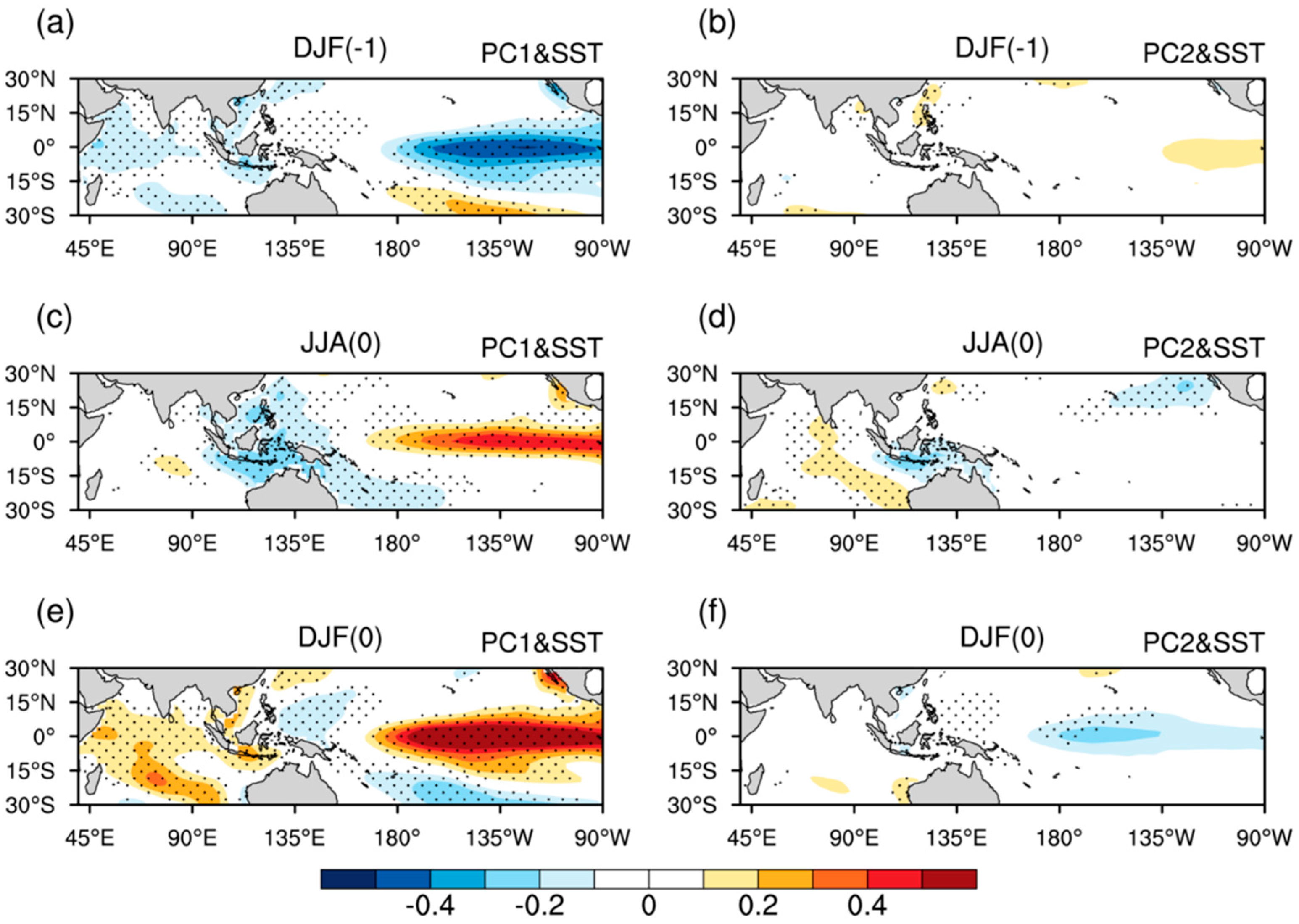
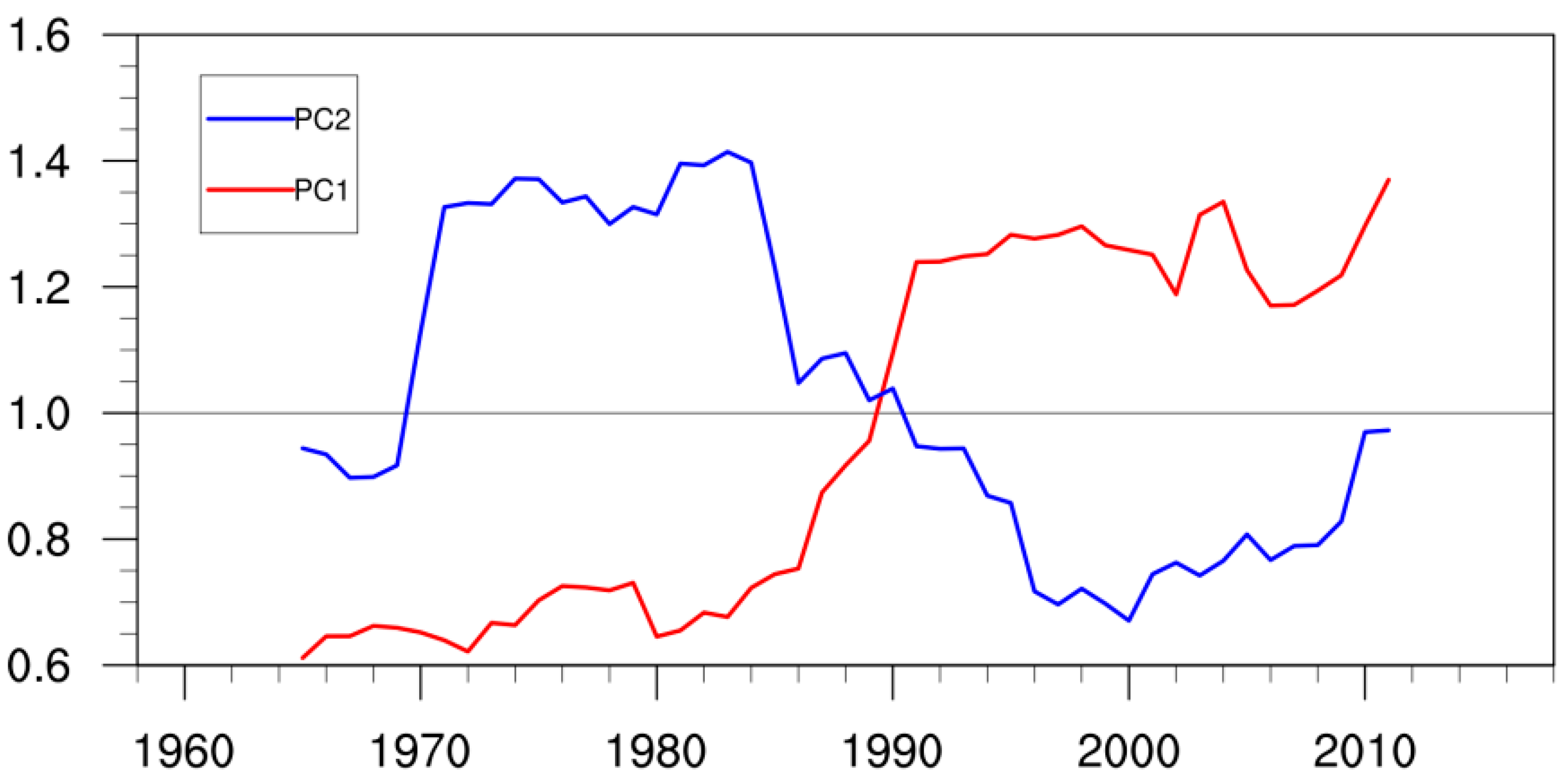
3. Characteristics of the Two Major Modes

In JJA, the water vapor source is mainly located in the southern hemisphere, and the water vapor sink is mainly located in the northern hemisphere [17,18], and thus the water vapor over the TEIOWP plays an important role in JJA precipitation anomalies over East Asia. According to Equations (1) and (2), we calculate the JJA–mean Q 2 for the period of 1958 to 2018 based on the NCEP/NCAR reanalysis data. To obtain the major modes of the water vapor source and sink anomalies over the TEIOWP, an empiric orthogonal function (EOF) is performed on the covariance matrix of the JJA–mean Q 2 anomalies over the TEIOWP for the period of 1958 to 2018 via the Equations (5)–(10). Figure 1a,b shows the spatial distribution of the first mode (EOF1) and the second mode (EOF2) of the water vapor source and sink anomalies over the TEIOWP (20° S–20° N, 90°–150° E). More than 25% and 12% of the total variance can be explained by the EOF1 and EOF2, which can be well separated from the other modes according to the “rule of thumb” [35]. In comparison, the accounted variances of the other modes are much smaller, and they can not be well separated from each other (figures not shown). The EOF1 mode presents a southwest-northeast oriented dipole with negative loading over the central-western maritime continent and positive loading over the northwestern Pacific (Figure 1a). Although the EOF2 mode presents five centers including two positive centers and three negative centers, the two centers over the southern South China sea (~110° E, 5° N) and the southeastern Bay of Bengal (~95° E, 10° N) are much weaker than the other three centers. The areas with strong loading in the EOF2 mode display a southwest-northeast oriented tripole, with one center over the eastern maritime continent and two centers with opposite signs over the western maritime continent and northwestern Pacific (Figure 1b). In other words, the out-of-phase linkage in water vapor source and sink between the western maritime continent and the northwestern Pacific in EOF1 mode is changed to in-phase linkage in EOF2 mode (Figure 1a vs. Figure 1b). Figure 1c,d shows the normalized principal components of the EOF1 (PC1) and EOF2 (PC2). Owing to the interdecadal component of Q 2 being removed, both the PC1 and PC2 present interannual variations.
Note that the water vapor source and sink are partly driven by horizontal winds, Figure 2 shows the JJA–mean water vapor flux anomalies and its divergence over the TEIOWP that associated with the PC1 and PC2. When the PC1 displays positive anomaly, the anomalous water vapor from the maritime continent transport northward and eastward to the northern tropical Indian Ocean and western tropical Pacific, respectively. Correspondingly, the water vapor divergence (convergence) over the central-western maritime continent (northwestern Pacific) agrees well with the dipole structure of the EOF1 mode (Figure 2a). In comparison, the water vapor anomalies associated with the PC2 is characterized by southeastward inflow from the maritime continent to the tropical Indian Ocean, and anticyclonic transport over the northwestern Pacific; the resultant divergence (convergence) over the western maritime continent and northwestern Pacific (eastern maritime continent) is consistent with the tripole structure of the EOF2 mode (Figure 2b). Thus, the distribution of water vapor source and sink anomalies in the two major modes are closely related to the water vapor divergence and convergence, respectively.
Furthermore, we investigate the role of vertical motion anomalies in contributing to the two major modes, as shown in Figure 3. Clearly, a South-North oriented dipole structure of the EOF1 mode is associated with an anomalous ascending branch at 10°–20° N and an anomalous descending branch at 0°–10° S, accompanying southerly winds anomalies and northerly winds anomalies over the lower troposphere and higher troposphere, respectively (Figure 3a). Similarly, a South-North oriented tripole structure of the EOF2 mode is associated with significant ascending motion anomalies over the 0°–10° N and descending motion anomalies over about 15° S and 20° N, with meridional winds converging and diverging over the lower troposphere and higher troposphere, respectively (Figure 3b). These results indicate that the single and double meridional cell anomalies mainly modulate the dipole structure of the EOF1 mode and tripole structure of the EOF2 mode, respectively.
To examine the linkage of evaporation and precipitation anomalies to the water vapor source and sink anomalies in the two major modes, the JJA–mean evaporation and precipitation slopes regressed against PC1 and PC2 are shown in Figure 4. The anomalous water vapor source over the central-western maritime continent in the EOF1 mode is associated with both the increase in evaporation and decrease of precipitation, whereas the anomalous water vapor sink over the northwestern Pacific is primarily associated with the increase in precipitation (Figure 4a,c). On the other hand, the increasing evaporation exerts a larger impact on the anomalous water vapor source over the western maritime continent in the EOF2 mode, but the precipitation anomalies play a major role in water vapor sink and source anomalies over the eastern maritime continent and northwestern Pacific (Figure 4b,d). Besides, the magnitude of the precipitation or evaporation anomalies associated with the PC1 are much larger than those associated with the PC2, where the PC1-related and PC2-related precipitation or evaporation anomalies over the TEIOWP areas are more (less) than 1.0 mm day−1 and 0.5 mm day−1, respectively (Figure 4a vs. Figure 4b; Figure 4c vs. Figure 4d). This suggests the EOF1 mode has a closer linkage with precipitation or evaporation anomalies over the TEIOWP than that of the EOF2 mode.

4. The Linkage between the External Forcings and the Two Major Modes

Previous studies reported that the sea surface temperature (SST) over the tropical Pacific and Indian Ocean are important external forcings affecting the interannual variability of water vapor over the TEIOWP [5,6,7,36]. To investigate the possible modulation effects of the external forcings on the two major modes, Figure 5 shows the regression of seasonal-mean SST slopes against PC1 and PC2 from the previous DJF (DJF(–1)) to the DJF. The positive phase of PC1 is associated with the significantly colder than normal SST over the central-eastern Pacific in the DJF(–1), while it transforms into a warmer state during JJA, and further strengthens during DJF (Figure 5a,c,e). The evolution of the SST anomalies over the central-eastern Pacific denotes a quick transition from the decaying La Niña phase to the developing El Niño phase. Correspondingly, the PC1 coincides well with the simultaneous Niño 3.4 index, and the linear correlation coefficient between them exceeds +0.59 (significant at the 99.9% confidence level). The significant in-phase linkage between the simultaneous Niño 3.4 index and PC1 is further supported by the scatterplot between them because more than three-quarters of the dots are located in the first and third quadrants (Figure 6a).
When the PC2 is in its positive phase, the SST anomalies in the DJF(–1) and the DJF are relatively weak and almost not significant, while the simultaneous SST is significantly warmer than normal over the tropical western Indian Ocean and colder than normal over the tropical southeastern Indian Ocean (Figure 5b,d,f), which corresponds to the positive phase of TIOD. The linear correlation coefficient between the PC2 and TIOD index exceeds +0.42 for the period of 1958 to 2018, and it is significant at the 99.9% confidence level. Again, the scatterplot between the simultaneous TIOD index and PC2 verifies the in-phase linkage between them, as evidenced by 45 out of 61 years presenting the same signs (Figure 6b). Therefore, the interannual variability of the PC1 and PC2 may be regulated by the quick transition of the ENSO phase and TIOD, respectively.

5. Discussion

The interannual variability of the PC1 is closely related to the quick transition of the ENSO phase, and it has pronounced pre-season tropical Pacific SST anomalies. Figure 7 shows the regression maps of the JJA–mean Q 2 , water vapor flux and meridional cell anomalies against the inverted DJF(–1) Niño 3.4 index. The distribution of Q 2 anomalies associated with the inverted Niño 3.4 index is similar to the EOF1 mode, with water vapor source anomalies over the central-western maritime continent and water vapor sink anomalies over the northwestern Pacific (Figure 1a vs. Figure 7a). The associated water vapor transport and convergence anomalies are also consistent with those associated with the PC1, which shows cyclonic transport and convergence over the northwestern Pacific, and northward transport and divergence over the central-western maritime continent (Figure 2a vs. Figure 7b). When the decaying La Niña is quickly transformed into the developing El Niño in JJA, the SST is colder than normal over the maritime continent, which favors suppressed convection aloft. The anomalous descending motion could excite an obvious “+, –” meridional wave train propagation resembling the Pacific-Japan pattern (Figure 7c) [3,37,38,39,40,41]. Meanwhile, an anomalous cyclone is triggered over the northwestern Pacific via the Indo-western Pacific Ocean capacitor effects (Figure 7b) [12,14,15]. These anomalies enhance the ascending motion and water vapor sink over the northwestern Pacific. Therefore, it is useful to predict the interannual variability of the PC1 base on the ENSO state in DJF(–1).
Note that PC2–TIOD index linkage is significant in JJA but not significant in the DJF(–1) (Figure 5b,d), we examine whether the EOF2 mode is affected by the TIOD via the lead-lag correlations between them, as shown in Figure 8. The in-phase linkage between the PC2 and TIOD index is not significant until June, as evidenced by the linear correlation coefficient between the TIOD index in May and PC is only +0.15, implying the TIOD is not an important precursor of EOF2 mode. Conversely, the significantly in-phase linkage between the PC2 and TIOD index during June–August is closely related to the significantly positive correlation between the PC2 and the tendency of the TIOD index during May–July, suggesting the TIOD is forced by PC2 to some extent (Figure 8). This is further supported by the evaporation anomalies associated with the PC2 being pronounced increased (decreased) over the tropical eastern (western) Indian Ocean (Figure 3b), which would induce the positive phase of TIOD via the wind-evaporation effect. As the interannual variability of the PC2 is not driven by TIOD or other SST modes, the EOF2 mode probably originates from internal atmospheric variability. This conclusion shares similarities with the results of Lu et al. [42] and He et al. [43], as the second mode of JJA WSPH resulting from internal atmospheric variability is underlined in their studies. On the other hand, although the EOF2 mode is not regulated by the ENSO, the standard deviation of PC2 is much lower in ENSO years (+0.79) compared to that in non-ENSO years (+1.09), which is opposite to the PC1 (+1.31 vs. +0.88). It is likely that the water source and sink anomalies over the TEIOWP tend to be dominant by EOF1 (EOF2) mode in ENSO (non-ENSO) years.
Compared to the period before the early 1990s, it is noteworthy that the amplitude of the PC1 is significantly enhanced after the early 1990s. In contrast, the amplitude of the PC2 is much lower after the early 1990s than that before the early 1990s (Figure 9). Correspondingly, although the loadings of the two major modes change are small over the whole period, the accounted variance of the dipole structure mode is increased from 14.8% to 35.7% between the two sub-periods of 1958 to 1990 and 1991 to 2018, whereas that of the tripole structure mode is decreased from 21.1% to 9.8% (Figure 10). Note that the external forcings, internal variability and change of the climate background may be responsible for the change of the PC1 and PC2 amplitude in the early 1990s, it is important to analyze the relative contribution of ENSO, internal variability and the global warming to this interdecadal change in future. Moreover, previous studies have shown that the water vapor source and sink over the TEIOWP is important to JJA precipitation anomalies over East Asia [5,6,7,14], but the impact of the water vapor source and sink over the TEIOWP on the JJA precipitation over East Asia has not been involved in the current study. Thus, future work needs to (1) analyze the underlying mechanism related to change of the PC1 and PC2 amplitude in the early 1990s; (2) investigate the relationship between the water vapor sink and source over the TEIOWP and the JJA precipitation anomalies over East Asia.

6. Summary

In this study, the interannual variability of the JJA–mean water vapor source and sink over the TEIOWP and the underlying mechanism are investigated by using the four-times daily and monthly-mean reanalysis datasets of NCEP/NCAR for the period of 1958 to 2018. The results show that nearly 40% of the total variance can be explained by the two major modes, which can be well separated from the other modes. The EOF1 mode and EOF2 mode of the water vapor source and sink anomalies over the TEIOWP present a southwest-northeast oriented dipole and a southwest-northeast oriented tripole, respectively. Specifically, the out-of-phase linkage in water vapor source and sink between the western maritime continent and the northwestern Pacific in EOF1 mode is changed to in-phase linkage in EOF2 mode. The water vapor anomalies associated with the PC1 (PC2) is characterized by northward transport from the maritime continent and (cyclonic) anticyclonic transport over the northwestern Pacific. The distribution of water vapor source and sink anomalies in the two major modes are closely related to the water vapor divergence and convergence, respectively. Corresponding to the in-phase and out-of-phase linkage between evaporation anomalies over the western maritime continent and precipitation anomalies over the northwestern Pacific, the single and double meridional cell anomalies mainly modulate the dipole structure of the EOF1 mode and tripole structure of EOF2 mode, respectively.
Moreover, the EOF1 mode is regulated by the quick transition of the ENSO phase, and it is useful to predict the associated PC1 based on the ENSO state in DJF(–1). When the decaying La Niña quickly transforms into the developing El Niño in the JJA, an obvious “+, –” meridional wave train resembling the Pacific-Japan pattern propagates from the tropics to the northwestern Pacific, which enhances the descending (ascending) motion and water vapor source (sink) over the western-central maritime continent (northwestern Pacific). In contrast, although the PC2 has a significant in-phase linkage with the simultaneous TIOD index, the EOF2 mode probably originates from internal atmospheric variability, as is evident from the SST anomalies over the tropical Indian Ocean are primarily forced by the EOF2 mode via the wind-evaporation effect. Additionally, owing to the standard deviation of PC1 is much higher in ENSO years than that in non-ENSO years, it is likely that the water source and sink anomalies over the TEIOWP tend to be dominant by EOF1 mode in ENSO years. In contrast, as the standard deviation of PC2 is much higher in non-ENSO years, the EOF2 mode may play an important role in water source and sink anomalies over the TEIOWP during non-ENSO years.

Author Contributions

Conceptualization, M.Z. and S.Q.; methodology, M.Z. and S.Q.; software, M.Z. and S.Q.; validation, M.Z., S.Q. and L.C.; formal analysis, M.Z. and S.Q.; investigation, M.Z. and S.Q.; resources, G.F., S.Q., C.H. and Q.L.; data curation, M.Z. and S.Q.; writing—original draft preparation, M.Z.; writing—review and editing, M.Z., S.Q., L.C., D.C. and C.H.; visualization, M.Z. and S.Q.; supervision, S.Q. All authors have read and agreed to the published version of the manuscript.

Funding

This study acknowledges the support of the Key Program of the National Natural Science Foundation of China (41530531), the National Key Research and Development Program of China (2017YFC1502301), the General Program of the National Natural Science Foundation of China (41905157, 41975088, 41975077) and the China Postdoctoral Science Foundation funded project (2018M640848).

Acknowledgments

We thank three anonymous reviewers for their constructive suggestions, which substantially improve our paper.

Conflicts of Interest

The authors declare no conflict of interest.

References

  1. Trenberth, K.E.; Fasullo, J. Water and energy budgets of hurricanes and implications for climate change. J. Geophys. Res. 2007, 112. [Google Scholar] [CrossRef]
  2. Bengtsson, L. The global atmospheric water cycle. Environ. Res. Lett. 2010, 5, 025202. [Google Scholar] [CrossRef]
  3. Qiao, Y.; Wu, R.; Huang, W.; Jian, M. Interannual variability of moisture source over southern Indian Ocean during boreal summer and its relationship with local SST. Int. J. Clim. 2013, 33, 556–567. [Google Scholar] [CrossRef]
  4. Simmonds, I.; Bi, D.; Hope, P. Atmospheric water vapor flux and its association with rainfall over China in summer. J. Clim. 1999, 12, 1353–1367. [Google Scholar] [CrossRef]
  5. Kawamura, R. A possible mechanism of the Asian summer monsoon-ENSO coupling. J. Meteor. Soc. Jap. 1998, 76, 1009–1027. [Google Scholar] [CrossRef] [Green Version]
  6. Webster, P.J.; Magana, V.O.; Palmer, T.N.; Shukla, J.; Tomas, R.A.; Yanai, M.; Yasunari, T. Monsoons: Processes, predictability, and the prospects for prediction. J. Geophys. Res. 1998, 103, 14451–14510. [Google Scholar] [CrossRef]
  7. Huang, R.H.; Chen, W.; Yang, B.L.; Zhang, R.H. Recent advances in studies of the interaction between the East Asian winter and summer monsoon and ENSO cycle. Adv. Atmos. Sci. 2004, 21, 407–424. [Google Scholar]
  8. Huang, R.H.; Lu, L. Numerical simulation of the relationship between the anomaly of subtropical high over East Asia and the convective activities in the western tropical Pacific. Adv. Atmos. Sci. 1989, 6, 202–214. [Google Scholar]
  9. Zhang, R.H.; Sumi, A.; Kimoto, M. A diagnostic study of the impact of El Nino on the precipitation in China. Adv. Atmos. Sci. 1999, 16, 229–241. [Google Scholar] [CrossRef]
  10. An, S.I.; Wang, B. Interdecadal change of the structure of the ENSO mode and its impact on the ENSO frequency. J. Clim. 2000, 13, 2044–2055. [Google Scholar] [CrossRef]
  11. Ding, Q.; Wang, B. Circumglobal teleconnection in the Northern Hemisphere summer. J. Clim. 2005, 18, 3483–3505. [Google Scholar] [CrossRef]
  12. Wang, B.; Wu, R.; Fu, X. Pacific–East Asian teleconnection: How does ENSO affect East Asian climate? J. Clim. 2000, 13, 1517–1536. [Google Scholar] [CrossRef]
  13. Yang, J.; Liu, Q.; Xie, S.P.; Liu, Z.; Wu, L. Impact of the Indian Ocean SST basin mode on the Asian summer monsoon. Geophys. Res. Lett. 2007, 34, L02708. [Google Scholar] [CrossRef] [Green Version]
  14. Xie, S.P.; Hu, K.; Hafner, J.; Tokinaga, H.; Du, Y.; Huang, G.; Sampe, T. Indian Ocean capacitor effect on Indo–western Pacific climate during the summer following El Niño. J. Clim. 2009, 22, 730–747. [Google Scholar] [CrossRef]
  15. Xie, S.P.; Kosaka, Y.; Du, Y.; Hu, K.; Chowdary, J.S.; Huang, G. Indo-western Pacific ocean capacitor and coherent climate anomalies in post-ENSO summer: A review. Adv. Atmos. Sci. 2016, 33, 411–432. [Google Scholar] [CrossRef] [Green Version]
  16. Zou, M.; Qiao, S.B.; Feng, T.C.; Wu, Y.P.; Feng, G.L. The inter–decadal change in anomalous summertime water vapour transport modes over the tropical Indian Ocean–western Pacific in the mid–1980s. Int. J. Clim. 2018, 38, 2672–2685. [Google Scholar] [CrossRef]
  17. Yanai, M.; Tomita, T. Seasonal and interannual variability of atmospheric heat sources and moisture sinks as determined from NCEP–NCAR reanalysis. J. Clim. 1998, 11, 463–482. [Google Scholar] [CrossRef] [Green Version]
  18. Qiao, Y.T.; Luo, H.B.; Jian, M.Q. The temporal and spatial characteristics of moisture budgets over Asian and Australian monsoon regions. J. Trop. Meteorol. 2002, 8, 113–120. [Google Scholar]
  19. Zhou, T.J.; Yu, R.C. Atmospheric water vapor transport associated with typical anomalous summer rainfall patterns in China. J. Geophys. Res. 2005, 110, D08104. [Google Scholar] [CrossRef] [Green Version]
  20. Li, X.Z.; Zhou, W.; Li, C.Y.; Song, J. Comparison of the annual cycles of moisture supply over southwest and southeast China. J. Clim. 2013, 26, 10139–10158. [Google Scholar] [CrossRef]
  21. Kalnay, E.; Kanamitsu, M.; Kistler, R.; Collins, W.; Deaven, D.; Gandin, L.; Iredell, M.; Saha, S.; White, G.; Woollen, J.; et al. The NCEP/NCAR 40-year reanalysis project. Bull. Am. Meteorol. Soc. 1996, 77, 437–472. [Google Scholar] [CrossRef] [Green Version]
  22. National Weather service. Climate Diagnostics Bulletin Updates to Climatologies and Indices Beginning with January 2011 Data. Available online: https://www.cpc.ncep.noaa.gov/data/indices/ (accessed on 30 December 2019).
  23. Huang, B.; Thorne, P.W.; Banzon, V.F.; Boyer, T.; Chepurin, G.; Lawrimore, J.H.; Menne, M.J.; Smith, T.M.; Vose, R.S.; Zhang, H.M. Extended reconstructed sea surface temperature, version 5 (ERSSTv5): Upgrades, validations, and intercomparisons. J. Clim. 2017, 30, 8179–8205. [Google Scholar] [CrossRef]
  24. Chen, M.; Xie, P.; Janowiak, J.E.; Arkin, P.A. Global land precipitation: A 50-yr monthly analysis based on gauge observations. J. Hydrometeorol. 2002, 3, 249–266. [Google Scholar] [CrossRef]
  25. Yu, L.; Weller, R.A. Objectively analyzed air–sea heat fluxes for the global ice-free oceans (1981–2005). Bull. Am. Meteorol. Soc. 2007, 88, 527–540. [Google Scholar] [CrossRef] [Green Version]
  26. Saji, N.H.; Goswami, B.N.; Vinayachandran, P.N.; Yamagata, T. A dipole mode in the tropical Indian Ocean. Nature 1999, 401, 360–363. [Google Scholar] [CrossRef]
  27. Yanai, M.; Esbensen, S.; Chu, J.H. Determination of bulk properties of tropical cloud clusters from large-scale heat and moisture budgets. J. Atmos. Sci. 1973, 30, 611–627. [Google Scholar] [CrossRef]
  28. Ciesielski, P.E.; Schubert, W.H.; Johnson, R.H. Large-Scale Heat and Moisture Budgets over the ASTEX Region. J. Atmos. Sci. 1999, 56, 3241–3261. [Google Scholar] [CrossRef]
  29. Obukhov, A.M. Statistically homogeneous fields on a sphere. Uspekhi Mat. Nauk. 1947, 2, 196–198. [Google Scholar]
  30. Fukuoka, A. A Study of 10-day Forecast (A Synthetic Report), Vol. XXII; The Geophysical Magazine: Tokyo, Japan, 1951; pp. 177–218. [Google Scholar]
  31. Lorenz, E.N. Empirical Orthogonal Functions and Statistical Weather Prediction; Technical Report, Statistical Forecast Project Report 1, Dep of Meteor, MIT Dept Meteorol, Sci Rept No 1; Statistical Forecasting Project Department of Meteorology: Cambridge, UK, 1956; p. 49. [Google Scholar]
  32. von Storch, H. Spatial Patterns: EOFs and CCA. In Analysis of Climate Variability: Application of Statistical Techniques; von Storch, H., Navarra, A., Eds.; Springer: Berlin, Germany, 1995; pp. 227–257. [Google Scholar]
  33. Wilks, D.S. Statistical Methods in the Atmospheric Sciences, 2nd ed.; Academic Press: Amsterdam, The Netherland, 2006. [Google Scholar]
  34. Hannachi, A. Pattern hunting in climate: A new method for finding trends in gridded climate data. Int. J. Clim. 2007, 27, 1–15. [Google Scholar] [CrossRef]
  35. North, G.R.; Bell, T.L.; Cahalan, R.F.; Moeng, F.J. Sampling errors in the estimation of empirical orthogonal functions. Mon. Weather Rev. 1982, 110, 699–706. [Google Scholar] [CrossRef]
  36. Hu, C.; Lian, T.; Cheung, H.N.; Qiao, S.; Li, Z.; Deng, K.; Yang, S.; Chen, D. Mixed diversity of shifting IOD and El Niño dominates the location of Maritime Continent autumn drought. Natl. Sci. Rev. 2020, 1–4. [Google Scholar] [CrossRef] [Green Version]
  37. Nitta, T. Convective activities in the tropical western Pacific and their impact on the Northern Hemisphere summer circulation. J. Meteor. Soc. Jap. Ser. II 1987, 65, 373–390. [Google Scholar] [CrossRef] [Green Version]
  38. Kosaka, Y.; Nakamura, H. Structure and dynamics of the summertime Pacific–Japan teleconnection pattern. Quart. J. Roy. Meteor. Soc. 2006, 132, 2009–2030. [Google Scholar] [CrossRef]
  39. Gong, H.N.; Wang, L.; Chen, W.; Wu, R.G.; Huang, G.; Nath, D. Diversity of the Pacific–Japan pattern among CMIP5 models: Role of SST anomalies and atmospheric mean flow. J. Clim. 2018, 31, 6857–6877. [Google Scholar] [CrossRef]
  40. Gong, Z.; Feng, G.; Dogar, M.M.; Huang, G. The possible physical mechanism for the EAP–SR co-action. Clim. Dyn. 2018, 51, 1499–1516. [Google Scholar] [CrossRef] [Green Version]
  41. Xu, P.; Wang, L.; Chen, W.; Feng, J.; Liu, Y. Structural changes in the Pacific–Japan pattern in the late 1990s. J. Clim. 2019, 32, 607–621. [Google Scholar] [CrossRef]
  42. Lu, R.; Li, Y.; Dong, B. External and Internal Summer Atmospheric Variability in the Western North Pacific and East Asia. J. Meteor. Soc. Jap. Ser. II 2006, 84, 447–462. [Google Scholar] [CrossRef] [Green Version]
  43. He, C.; Zhou, T.; Zou, L.; Zhang, L. Two interannual variability modes of the Northwestern Pacific Subtropical Anticyclone in boreal summer. Sci. China Earth Sci. 2013, 56, 1254–1265. [Google Scholar] [CrossRef]
Figure 1. (a,b) The first and second eigenvectors (EOF1, EOF2) of JJA–mean Q 2 anomalies over the tropical eastern Indian Ocean-western Pacific (TEIOWP) for the period of 1958 to 2018; (c,d) the corresponding normalized time series (PC1 and PC2). The explained variance is indicated at the top right; the zero contours are omitted.
Atmosphere 11 00758 g001
Figure 2. (a) Linear regression slopes of JJA–mean water vapor flux (vector; kg m−1s−1) and the associated divergence (shaded; 10−7 g m−2 s−1) at each grid of the TEIOWP onto the PC1 for the period of 1958 to 2018. (b) As in (a), but for PC2. Only the water vapor flux anomalies that were significant at the 95% confidence level are plotted.
Atmosphere 11 00758 g002
Figure 3. (a) Linear regression slopes of the latitude–height cross-section of the JJA–mean vertical velocity (contour interval; 100−1 Pa s−1), wind (vector; meridional component, m s−1; vertical component, Pa s−1, multiplied by –100; the wind speeds less than 0.1 m s−1 are not shown) averaged over 110°–140° E at each grid onto the PC1 for the period of 1958 to 2018. (b) As in (a), but for PC2. Note that the unit of the Y-axis is hPa. The shaded area denotes the wind anomalies exceeding the 95% confidence level; the zero contours are omitted.
Atmosphere 11 00758 g003
Figure 4. Linear regression slopes of JJA–mean (a) precipitation (shaded; mm day−1) and (c) evaporation (shaded; mm day−1) at each grid of TEIOWP onto the PC1 for the period of 1958 to 2018. (b,d) As in (a,c) but for PC2. The black dotted area exceeds the 95% significance level.
Atmosphere 11 00758 g004
Figure 5. Linear regression slopes of SST (shaded; °C) over the tropical Indian Ocean and Pacific in the (a) DJF(–1), (c) JJA and (e) DJF onto PC1. (b,d,f) As in (a,c,e), but for PC2. The black dotted area exceeds the 95% confidence level.
Atmosphere 11 00758 g005
Figure 6. (a) Scatterplot of the normalized time series of JJA–mean Niño3.4 index and PC1. (b) As in (a), but for the JJA–mean TIOD index and PC2. The correlation between the two time series is shown at the top.
Atmosphere 11 00758 g006
Figure 7. Linear regression slopes of JJA–mean (a) Q 2 (shaded; W m−2), (b) water vapor flux (vector; kg m−1s−1) and divergence (shaded; 10−7 g m−2 s−1) at each grid of TEIOWP, and (c) vertical velocity (contour interval; 100−1 Pa s−1) and wind (vector; meridional component, m s−1; vertical component, Pa s−1, multiplied by -100; the wind speeds less than 0.1 m s−1 are not shown) averaged over 110°–140° E at each grid onto the inverted DJF(–1)–mean Niño3.4 index for the period of 1958 to 2018. Note that the units of the Y-axis in (c) is hPa. The black dotted area in (a) denotes the Q2 anomalies exceeding the 95% significance level, respectively. The shaded area in (c) denotes the wind anomalies exceeding the 95% confidence level; the zero contours are omitted. Only the water vapor flux anomalies significant at the 95% confidence level are plotted in (b).
Atmosphere 11 00758 g007
Figure 8. Lag–lead correlation between monthly TIOD indices and PC2 (black line), and between the tendency of monthly TIOD indices and PC2 (red line) for the period of 1958 to 2018. The dashed line denotes the 95% confidence level.
Atmosphere 11 00758 g008
Figure 9. The 15-year running standard deviation of PC1 (red line) and PC2 (blue line) for the period of 1958 to 2018. The years on abscissa are the central year of the 15-year window.
Atmosphere 11 00758 g009
Figure 10. (a,b) The first and second eigenvectors (EOF1, EOF2) of JJA–mean Q 2 anomalies over the TEIOWP for the period of 1958 to 1990; (c,d) as in (a,b), but for the period of 1991 to 2018. The explained variance is indicated at the top right; the zero contours are omitted.
Atmosphere 11 00758 g010

