Evaluation of WRF-Chem Predictions for Dust Deposition in Southwestern Iran


Abstract
:1. Introduction
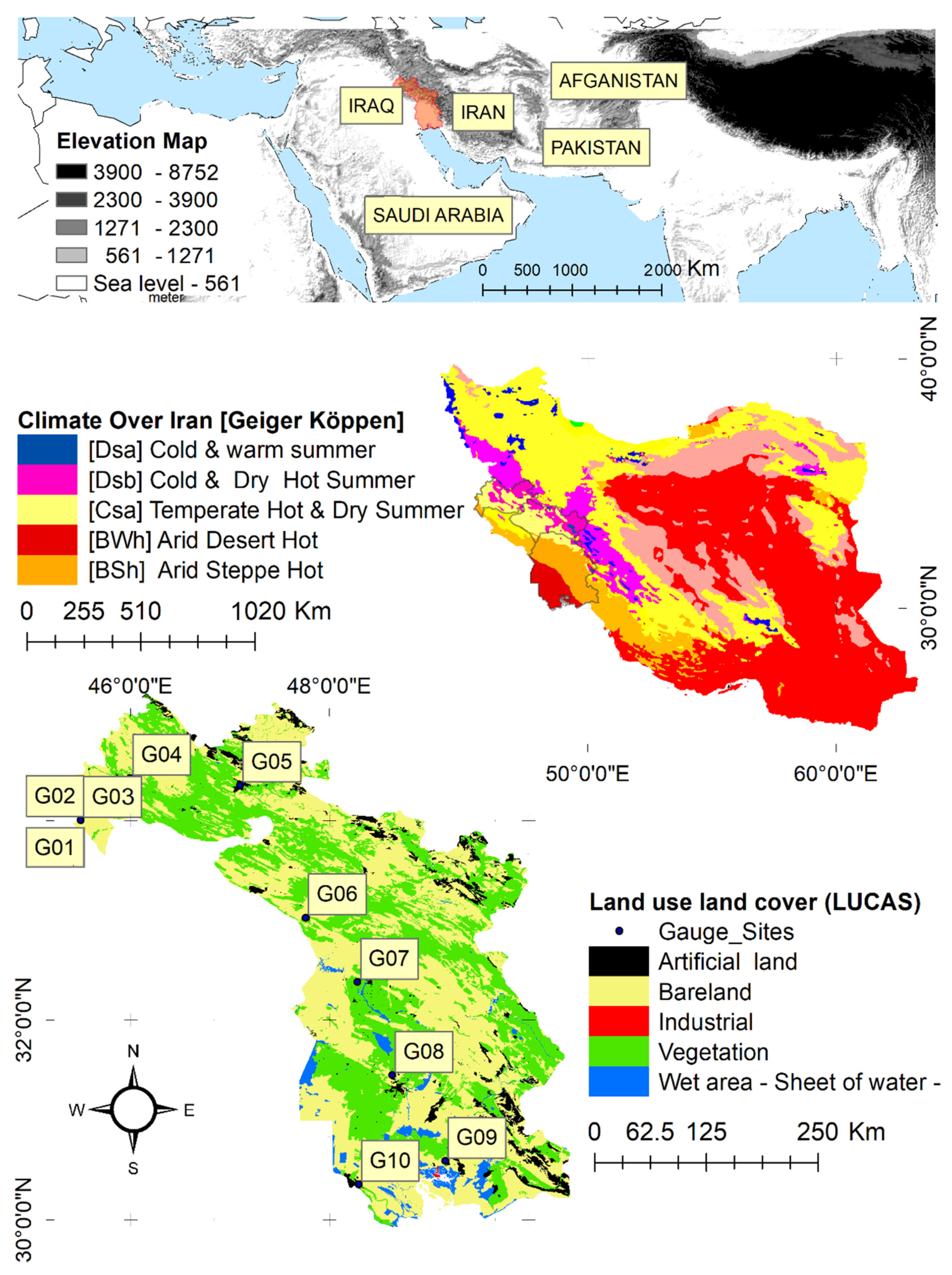
2. Study Area
2.1. Setting Sites and Data
2.2. Climatic Characteristics
3. Approaches and Methodology
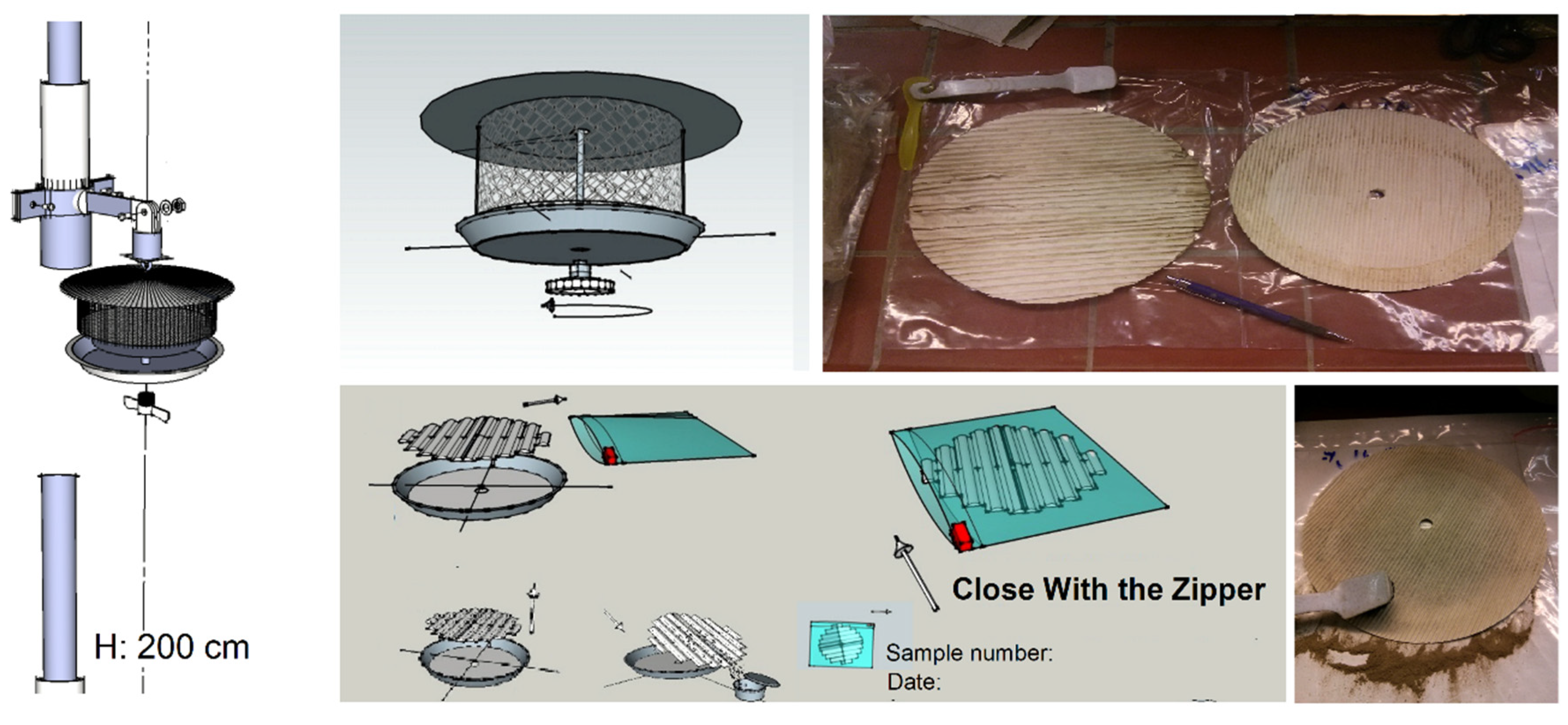
3.1. Ground Observation, Sites and Sampling
3.1.1. Data Sampling Method and Analysis
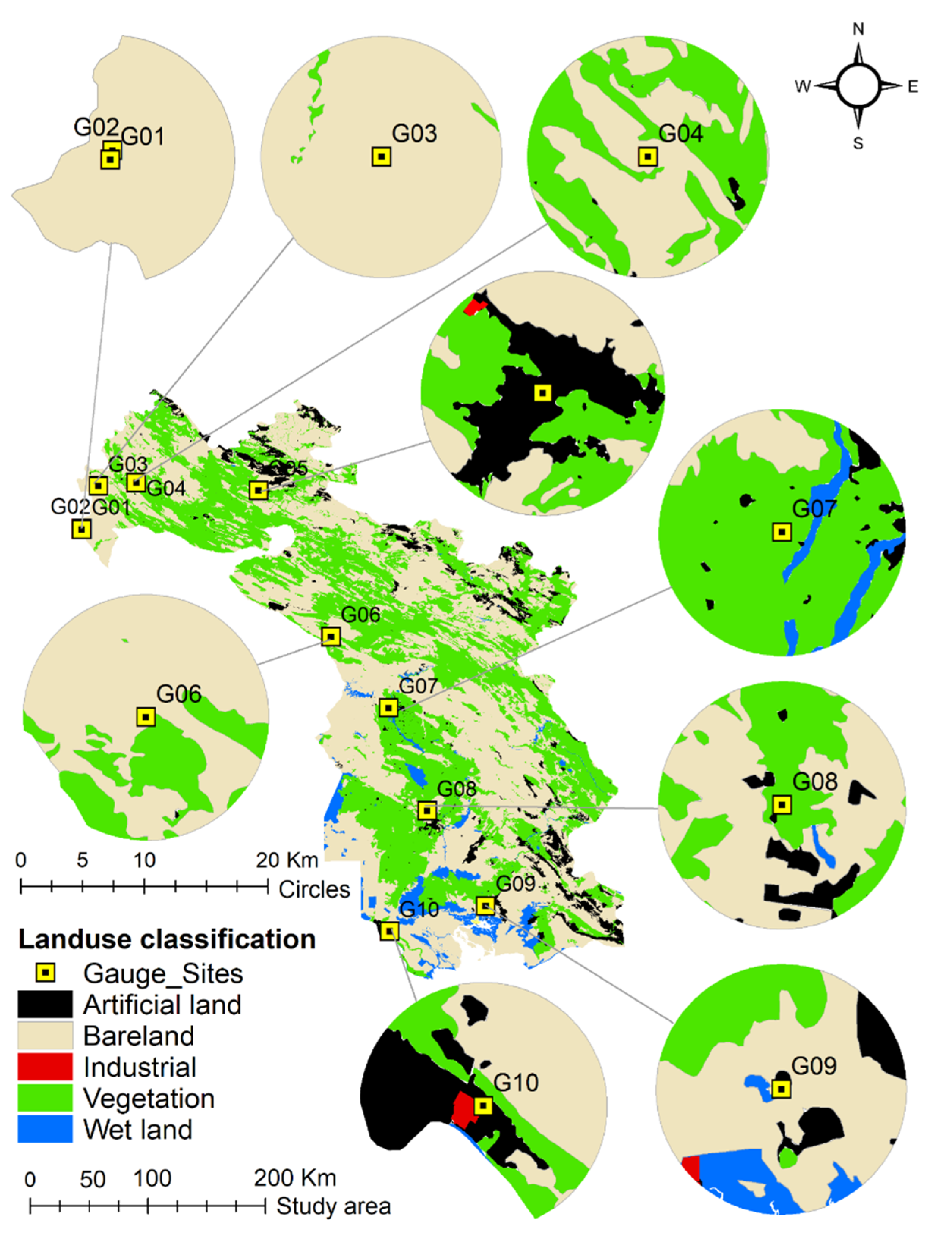
3.1.2. LULC on the Gauge Sites
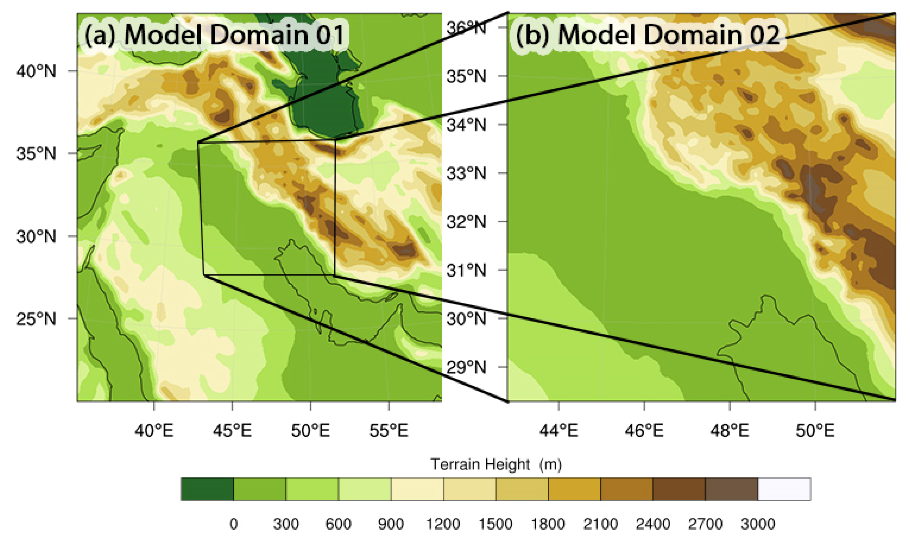
3.2. Setting WRF-Chem Model Simulation
4. Results
4.1. Experiment, Sites and Sampling Result
4.1.1. Climate and LULC for Each Site
4.1.2. Meteorological Data
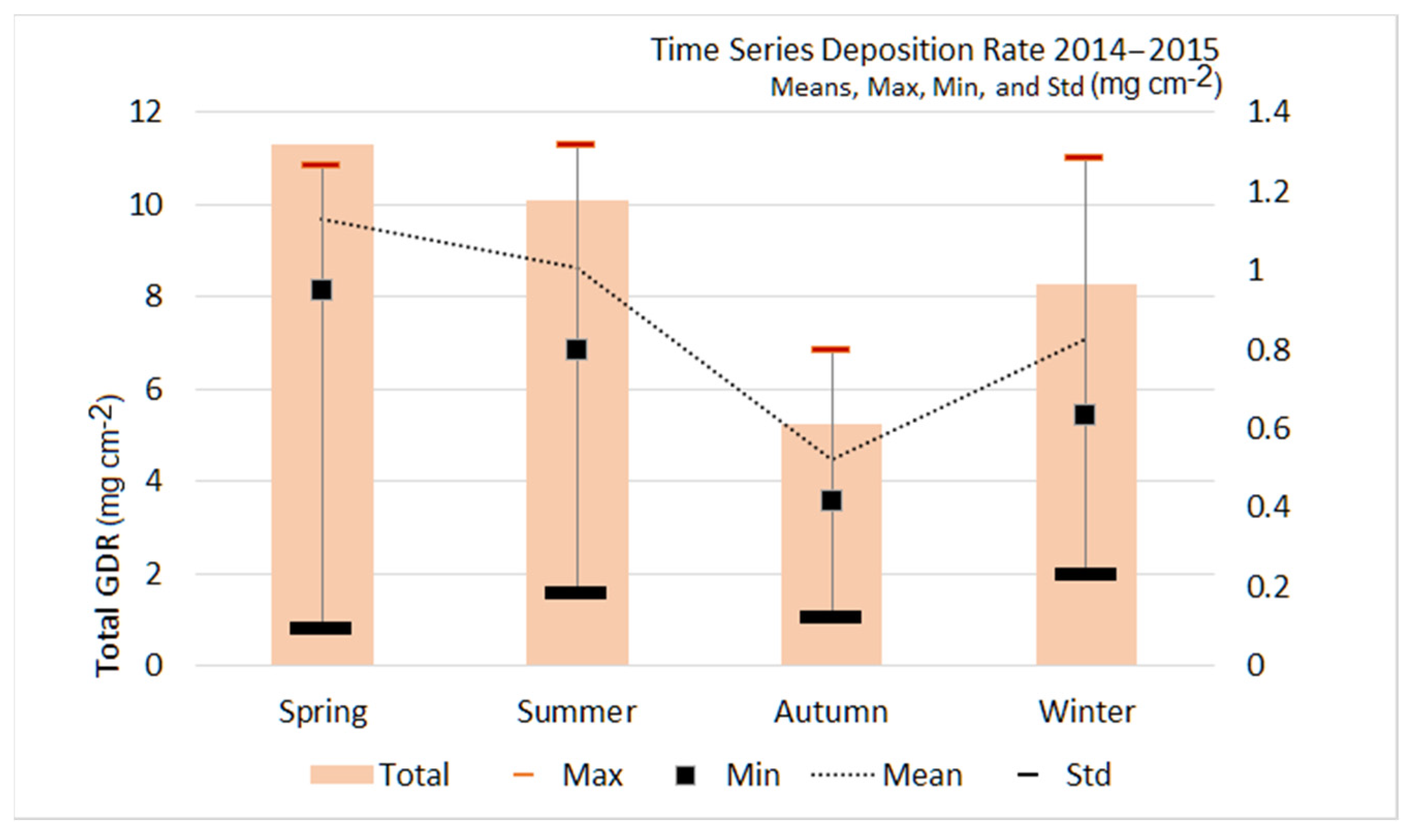
4.1.3. Dust Sampling Analysis
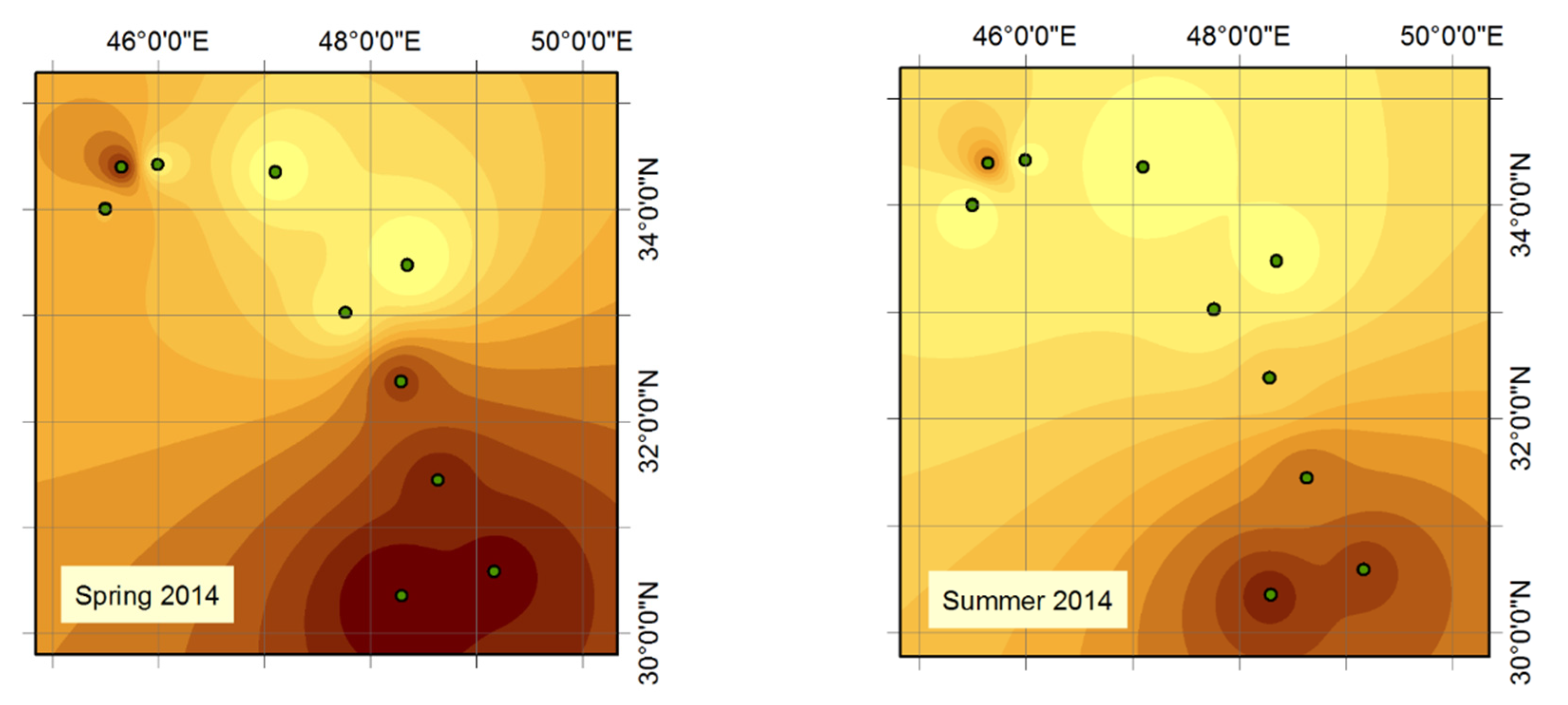
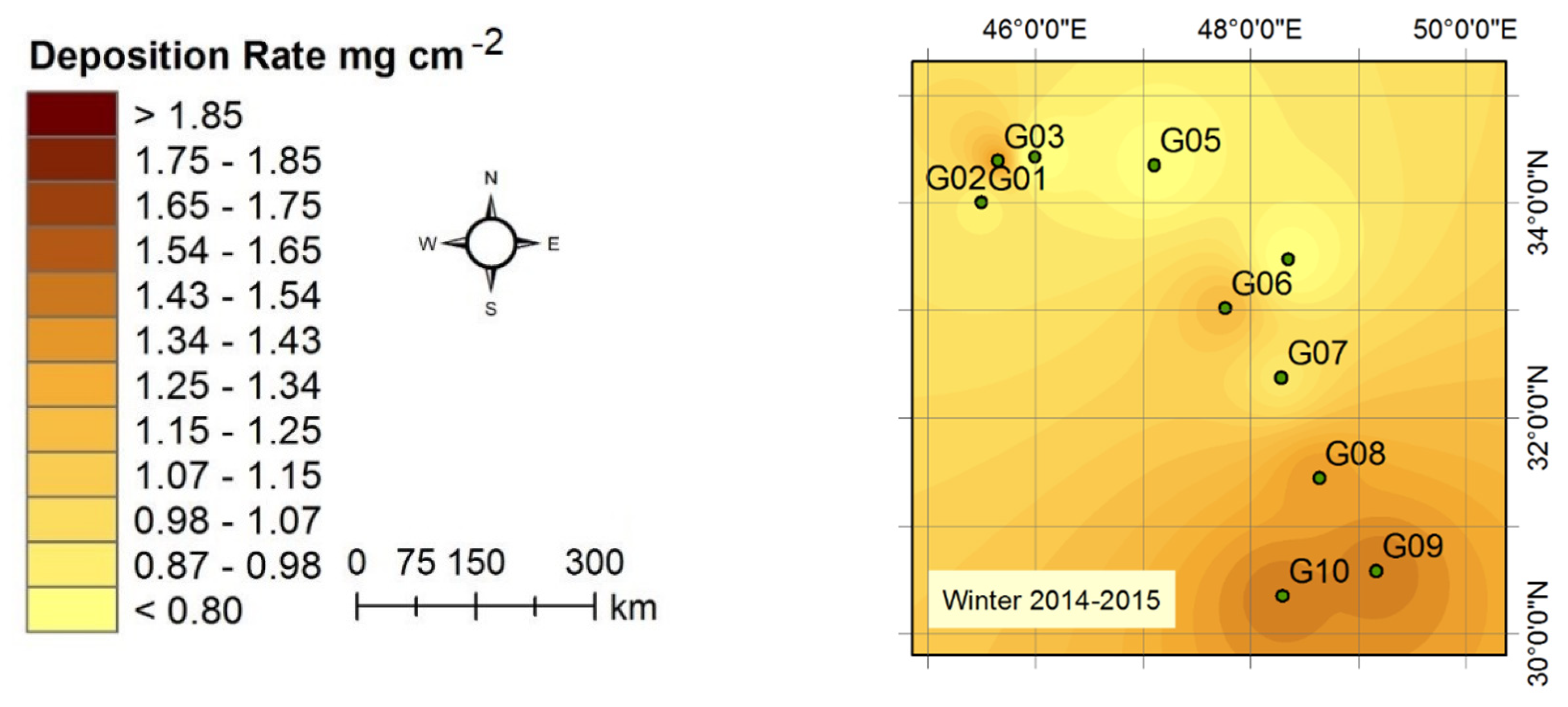
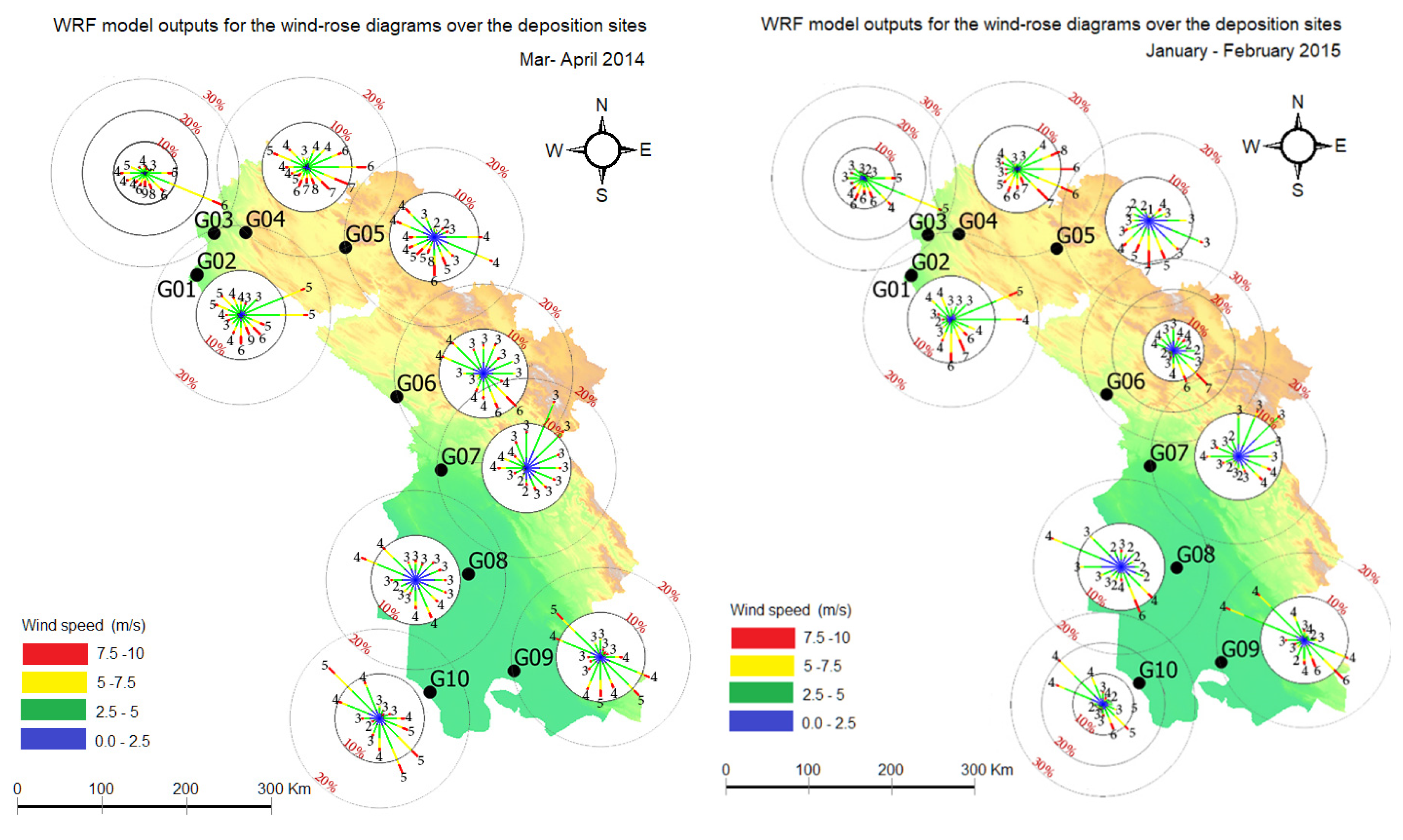
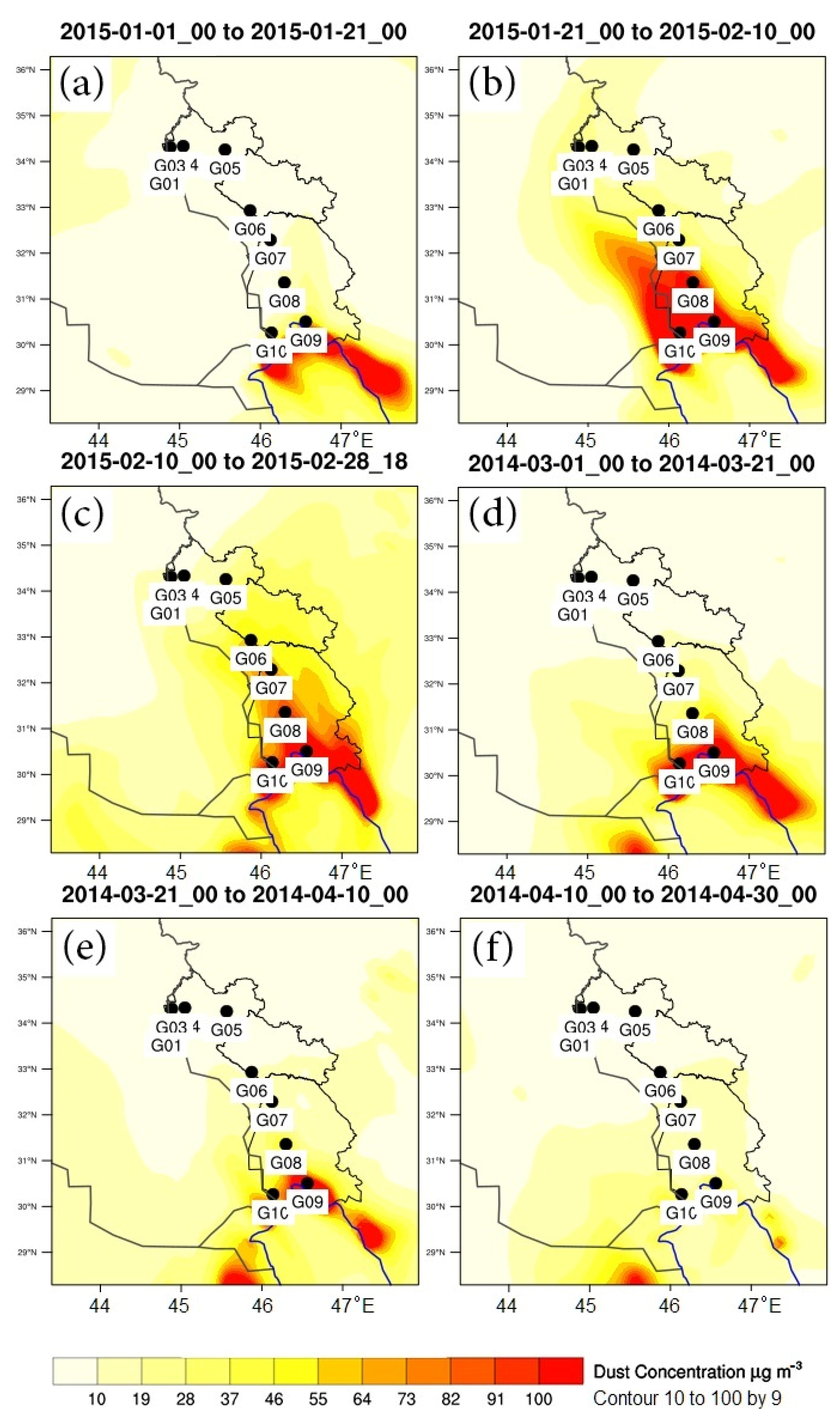
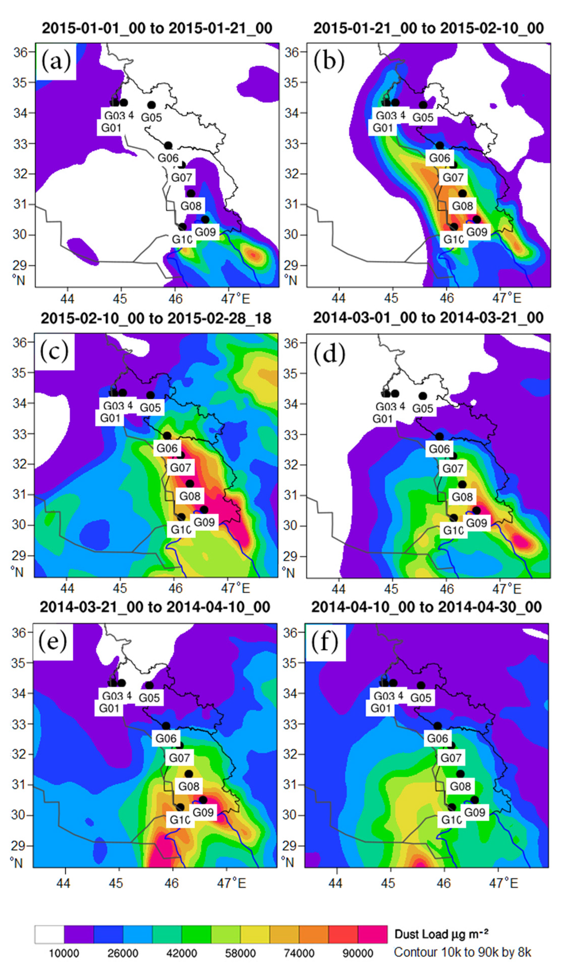
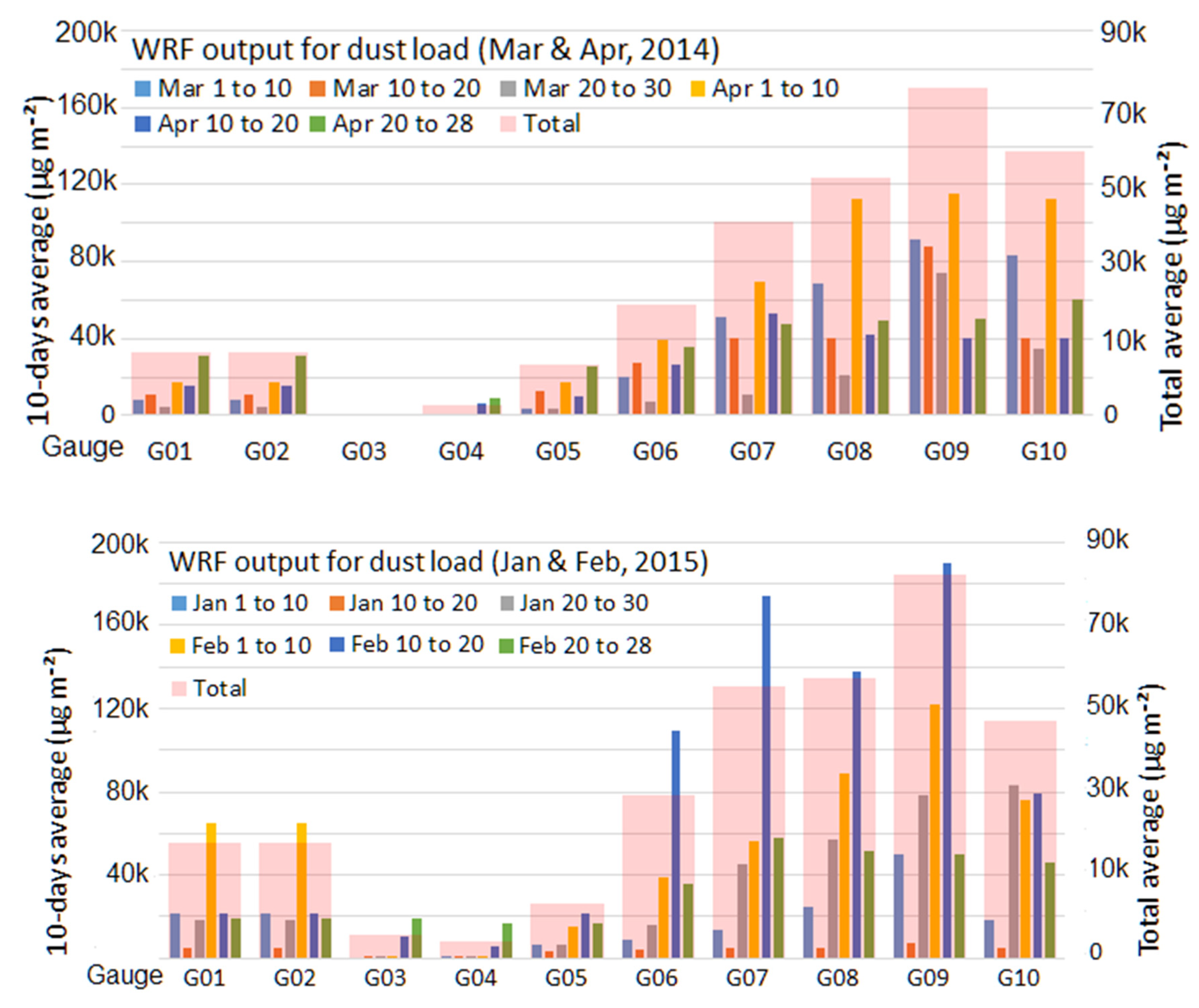
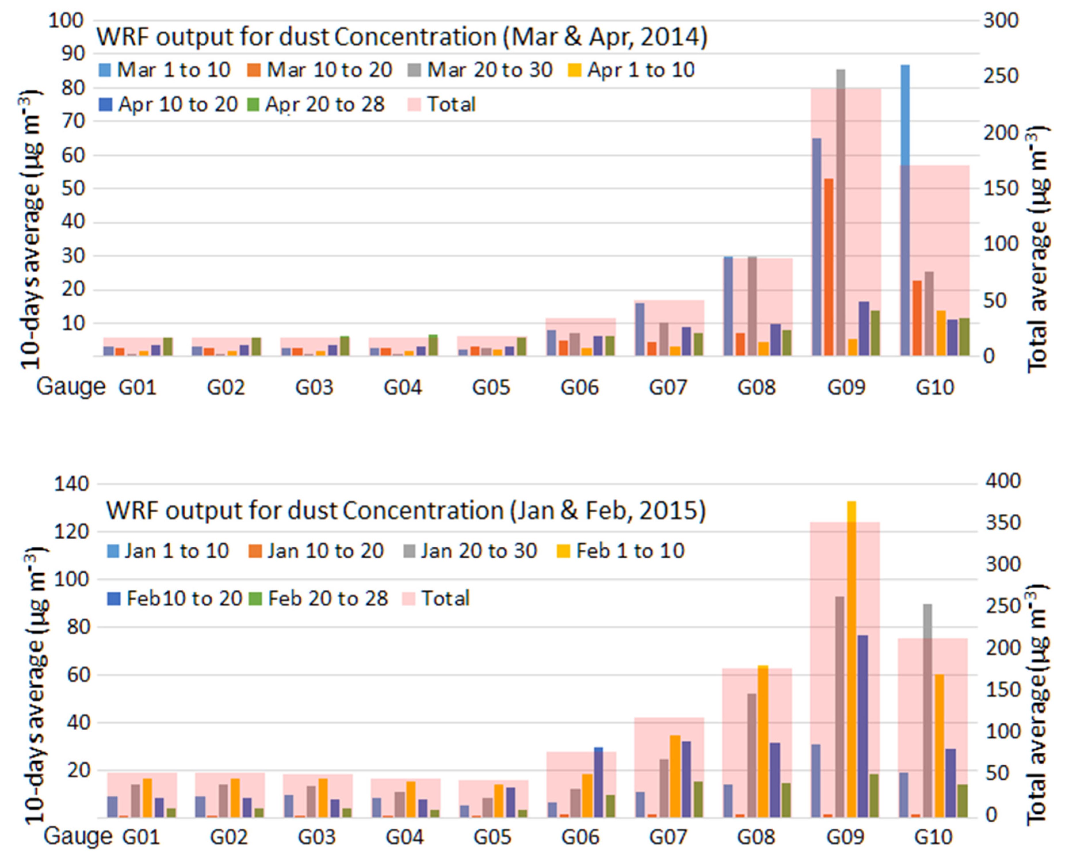
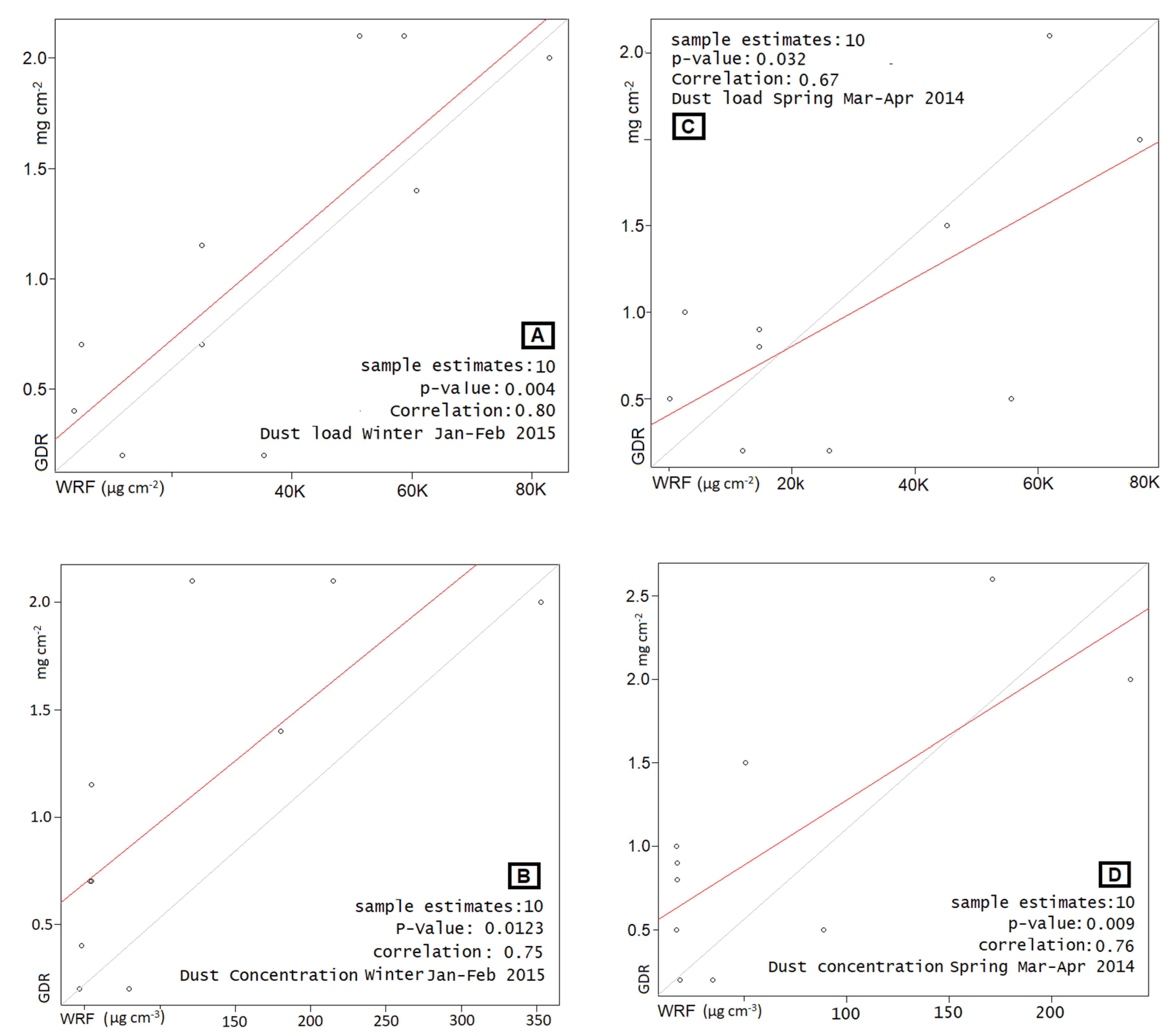
4.2. WRF-Chem Model Output
5. Discussion
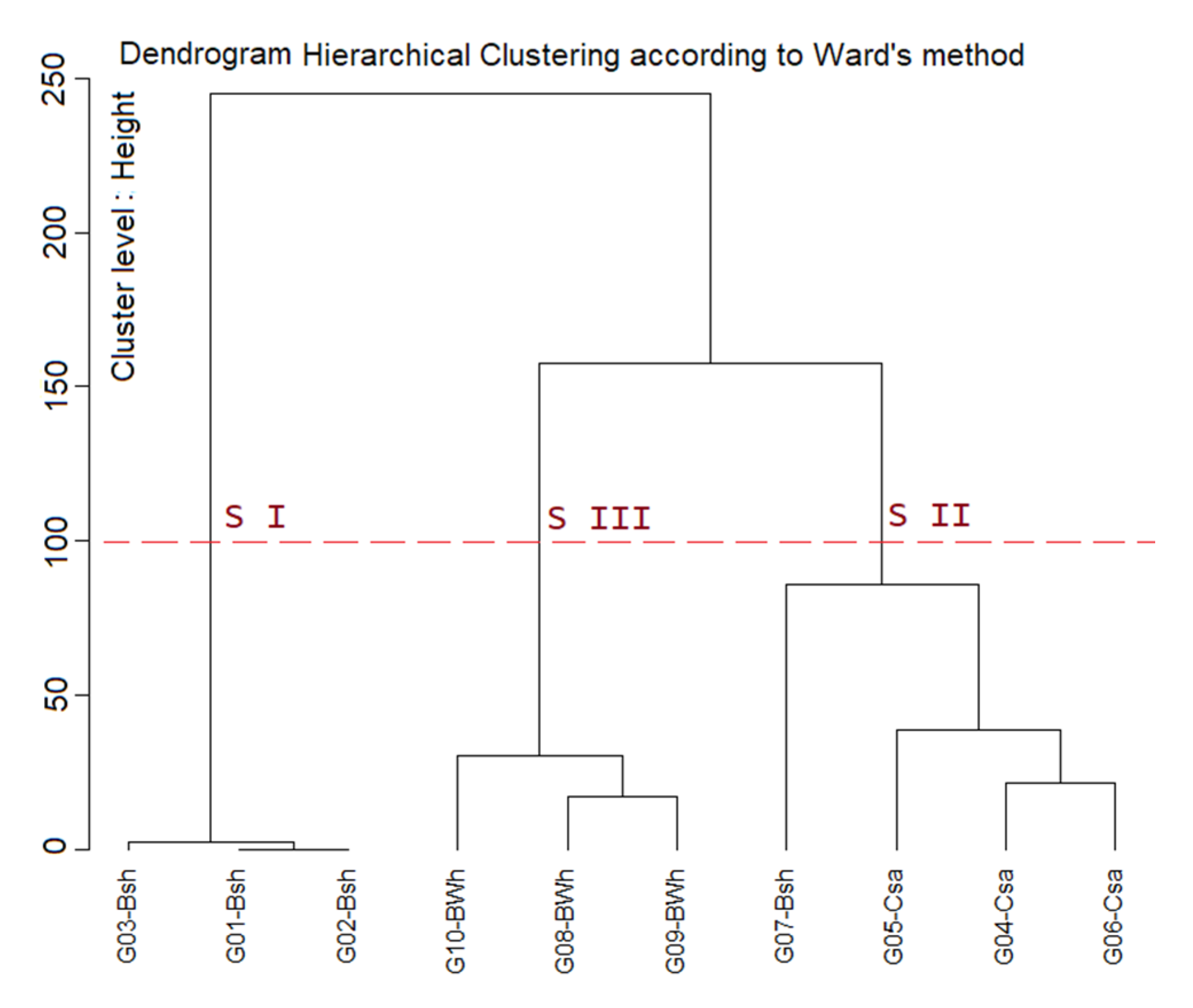
5.1. Field Experiment and Classification Part of Discussion
5.2. Model Combined in Each Site and Scenario
5.3. Finding and Importance of Ground Deposition
6. Conclusions
Author Contributions
Funding
Acknowledgments
Conflicts of Interest
References
- Gold, V.; Loening, K.L.; McNaught, A.D.; Shemi, P.; Wilkinson, A. Glossary of atmospheric chemistry terms. Pure Appl. Chem. 1990, 62, 2167–2219. [Google Scholar]
- Charlson, R.; Schwartz, S.E.; Hales, J.M.; Cess, R.D.; Coakley, J.J.; Hansen, J.E.; Hofmann, D.J. Climate forcing by anthropogenic aerosols. Science 1992, 255, 423–430. [Google Scholar] [CrossRef]
- Prospero, J.M.; Ginoux, P.; Torres, O.; Nicholson, S.E.; Gill, T.E. Environmental characterization of global sources of atmospheric soil dust identified with the Nimbus 7 Total Ozone Mapping Spectrometer (TOMS) absorbing aerosol product. Rev. Geophys. 2002, 40, 2–31. [Google Scholar] [CrossRef]
- Tegen, I.; Werner, M.; Harrison, S.P.; Kohfeld, K.E. Relative importance of climate and land use in determining present and future global soil dust emission. Geophys. Res. Lett. 2004, 31, 5. [Google Scholar] [CrossRef] [Green Version]
- Amiridis, V.; Wandinger, U.; Marinou, E.; Giannakaki, E.; Tsekeri, A.; Basart, S.; Kazadzis, S.; Gkikas, A.; Taylor, M.; Baldasano, J.; et al. Optimizing CALIPSO Saharan dust retrievals. Atmos. Chem. Phys. 2013, 13, 12089–12106. [Google Scholar] [CrossRef] [Green Version]
- Chen, Y.S.; Sheen, P.C.; Chen, E.R.; Liu, Y.K.; Wu, T.N.; Yang, C.Y. Effects of Asian dust storm events on daily mortality in Taipei, Taiwan. Environ. Res. 2004, 95, 151–155. [Google Scholar] [CrossRef]
- Groll, M.; Opp, C.; Aslanov, I. Spatial and temporal distribution of the dust deposition in Central Asia–results from a long term monitoring program. Aeolian Res. 2013, 9, 49–62. [Google Scholar] [CrossRef]
- Opp, C.; Groll, M.; Aslanov, I.; Lotz, T.; Vereshagina, N. Aeolian dust deposition in the southern Aral Sea region (Uzbekistan): Ground-based monitoring results from the LUCA project. Quat. Int. 2017, 429, 86–99. [Google Scholar] [CrossRef]
- Stefanski, R.; Sivakumar, M.V.K. Impacts of sand and dust storms on agriculture and potential agricultural applications of a SDSWS. In Proceedings of the IOP Conference Series: Earth and Environmental Science, Bristol, UK, March 2009; Available online: https://iopscience.iop.org/article/10.1088/1755-1307/7/1/012016 (accessed on 18 June 2020).
- Ohde, T.; Siegel, H. Impacts of Saharan dust and clouds on photosynthetically available radiation in the area off Northwest Africa. Tellus Ser. B-Chem. Phys. Meteorol. 2012, 64, 17160. [Google Scholar] [CrossRef] [Green Version]
- Schepanski, K.; Heinold, B.; Tegen, I. Harmattan, Saharan. heat low, and West African monsoon circulation: Modulations on the Saharan dust outflow towards the North Atlantic. Atmos. Chem. Phys. 2017, 17, 10223–10243. [Google Scholar] [CrossRef] [Green Version]
- Skamarock, W.; Klemp, J.; Dudhia, J.; Gill, D.; Barker, D.; Duda, M.; Powers, J. Description of the Advanced Research WRF Version 3; National Center for Atmospheric Research Technical: Boulder, CO, USA, June 2008. [Google Scholar]
- Mandal, M.; Mohanty, U.C.; Raman, S. A study on the impact of parameterization of physical processes on prediction of tropical cyclones over the Bay of Bengal with NCAR/PSU mesoscale model. Nat. Hazards 2004, 31, 391–414. [Google Scholar] [CrossRef]
- Carvalho, D.; Rocha, A.; Gómez-Gesteira, M.; Santos, C.S. WRF wind simulation and wind energy production estimates forced by different reanalyses: Comparison with observed data for Portugal. Appl. Energy 2014, 117, 116–126. [Google Scholar] [CrossRef]
- Li, N.; Long, X.; Tie, X.; Cao, J.; Huang, R.; Zhang, R.; Feng, T.; Liu, S.; Li, G. Urban dust in the Guanzhong basin of China, part II: A case study of urban dust pollution using the WRF-Dust model. Sci. Total Environ. 2016, 541, 1614–1624. [Google Scholar] [CrossRef] [PubMed]
- Hahnenberger, M.; Nicoll, K. Geomorphic and land cover identification of dust sources in the eastern Great Basin of Utah, USA. Geomorphology 2014, 204, 657–672. [Google Scholar] [CrossRef]
- Huang, J.; Wang, T.; Wang, W.; Li, Z.; Yan, H. Climate effects of dust aerosols over East Asian arid and semiarid regions. J. Geophys. Res. Atmos. 2014, 119, 11398–11416. [Google Scholar] [CrossRef]
- Chen, B.; Stein, A.F.; Maldonado, P.G.; de la Campa, A.M.S.; Gonzalez-Castanedo, Y.; Castell, N.; Jesus, D. Size distribution and concentrations of heavy metals in atmospheric aerosols originating from industrial emissions as predicted by the HYSPLIT model. Atmos. Environ. 2013, 71, 234–244. [Google Scholar] [CrossRef]
- Nabavi, S.O.; Haimberger, L.; Samimi, C. Sensitivity of WRF-chem predictions to dust source function specification in West Asia. Aeolian Res. 2017, 24, 115–131. [Google Scholar] [CrossRef]
- Chen, S.; Zhao, C.; Qian, Y.; Leung, L.R.; Huang, J.; Huang, Z.; Bi, J.; Zhang, W.; Shi, J.; Yang, L.; et al. Regional modeling of dust mass balance and radiative forcing over East Asia using WRF-Chem. Aeolian Res. 2014, 15, 15–30. [Google Scholar] [CrossRef]
- Huang, J.; Minnis, P.; Yan, H.; Yi, Y.; Chen, B.; Zhang, L.; Ayers, J.K. Dust aerosol effect on semi-arid climate over Northwest China detected from A-Train satellite measurements. Atmos. Chem. Phys. 2010, 10, 6863–6872. [Google Scholar] [CrossRef] [Green Version]
- Beres, J.H.; Garcia, R.R.; Boville, B.A.; Sassi, F. Implementation of a gravity wave source spectrum parameterization dependent on the properties of convection in the Whole Atmosphere Community Climate Model (WACCM). J. Geophys. Res. Atmos. 2005, 110. [Google Scholar] [CrossRef] [Green Version]
- Koren, I.; Kaufman, Y.J.; Washington, R.; Todd, M.C.; Rudich, Y.; Martins, J.V.; Rosenfeld, D. The Bodélé depression: A single spot in the Sahara that provides most of the mineral dust to the Amazon forest. Environ. Res. Lett. 2006, 1. [Google Scholar] [CrossRef]
- Todd, M.C.; Bou Karam, D.; Cavazos, C.; Bouet, C.; Heinold, B.; Baldasano, J.M.; Cautenet, G.; Koren, I.; Perez, C.; Solmon, F.; et al. Quantifying uncertainty in estimates of mineral dust flux: An intercomparison of model performance over the Bodélé Depression, northern Chad. J. Geophys. Res. Atmos. 2008, 113. [Google Scholar] [CrossRef] [Green Version]
- Bullard, J.E.; Harrison, S.P.; Baddock, M.C.; Drake, N.; Gill, T.E.; McTainsh, G.; Sun, Y. Preferential dust sources: A geomorphological classification designed for use in global dust-cycle models. J. Geophys. Res. Earth Surf. 2011, 116. [Google Scholar] [CrossRef] [Green Version]
- Ginoux, P.; Chin, M.; Tegen, I.; Prospero, J.M.; Holben, B.; Dubovik, O.; Lin, S.J. Sources and distributions of dust aerosols simulated with the GOCART model. J. Geophys. Res. Atmos. 2001, 106, 20255–20273. [Google Scholar] [CrossRef]
- Rashki, A.; Eriksson, P.G.; Rautenbach, C.D.W.; Kaskaoutis, D.G.; Grote, W.; Dykstra, J. Assessment of chemical and mineralogical characteristics of airborne dust in the Sistan region, Iran. Chemosphere 2013, 90, 227–236. [Google Scholar] [CrossRef] [Green Version]
- Foroushani, M.A.; Opp, C.; Groll, M. Chemical Characterization of Aeolian Dust Deposition in Southern and Western Iran. Asian J. Geogr. Res. 2019, 2, 1–22. [Google Scholar] [CrossRef] [Green Version]
- Goudie, A.S.; Middleton, N.J. Saharan dust storms: Nature and consequences. Earth-Sci. Rev. 2001, 56, 179–204. [Google Scholar] [CrossRef]
- Schleicher, N.J.; Norra, S.; Chai, F.; Chen, Y.; Wang, S.; Cen, K.; Yu, Y.; Stüben, D. Temporal variability of trace metal mobility of urban particulate matter from Beijing–A contribution to health impact assessments of aerosols. Atmos. Environ. 2011, 45, 7248–7265. [Google Scholar] [CrossRef]
- Choobari, O.A.; Zawar-Reza, P.; Sturman, A. Feedback between windblown dust and planetary boundary-layer characteristics: Sensitivity to boundary and surface layer parameterizations. Atmos. Environ. 2012, 61, 294–304. [Google Scholar] [CrossRef]
- Global Ambient Air Pollution, World Health Organization. 2018. Available online: https://www.who.int/quantifying_ehimpacts/global/source_apport/en/ (accessed on 18 June 2020).
- Almasi, A.; Mousavi, A.R.; Bakhshi, S.; Namdari, F. Dust storms and environmental health impacts. J. Middle East Appl. Sci. Technol. 2014, 8, 353–356. [Google Scholar]
- Peel, M.C.; Finlayson, B.L.; McMahon. Updated world map of the Köppen-Geiger climate classification. Hydrol. Earth Syst. Sci. 2007, 11, 1633–1644. [Google Scholar] [CrossRef] [Green Version]
- Iran Meteorological Organization. Precipitation Map. 2014. Available online: http://www.irimo.ir/index.php?newlang=eng (accessed on 25 January 2014).
- NASA; METI; AIST; Japan Spacesystems; US/Japan ASTER Science Team. ASTER Global Digital Elevation Model (GDEM). 2001. Available online: https://doi.org/10.5067/aster/ast14dem.003 (accessed on 15 December 2017).
- Russell, R. Dry Climates of the United States. Part I; The Climatic Map. Univ. of California; University of California Press: Berkeley, CA, USA, 1931. [Google Scholar]
- Kriticos, D.J.; Webber, B.L.; Leriche, A.; Ota, N.; Macadam, I.; Bathols, J.; Scott, J.K. CliMond: Global high-resolution historical and future scenario climate surfaces for bioclimatic modelling. Methods Ecol. Evol. 2012, 3, 56–64. [Google Scholar] [CrossRef]
- IHS under License with ASTM. “Standard Terminology Relating to Sampling and Analysis of Atmospheres,” IHS License ASTM. 2010. Available online: https://wenku.baidu.com/view/8324a4b765ce050876321358 (accessed on 27 January 2014).
- ASTM D1356, Standard Terminology Relating to Sampling and Analysis of Atmospheres, Subcommittee D22.03. 2017. Available online: https://standards.globalspec.com/std/10195132/ASTM%20D1356 (accessed on 15 December 2017).
- Parsa, V.A.; Yavari, A.; Nejadi, A. Spatio-temporal analysis of land use/land cover pattern changes in Arasbaran Biosphere Reserve: Iran. Model. Earth Syst. Environ. 2016, 2, 1–13. [Google Scholar] [CrossRef]
- Verburg, P.H.; Schot, P.P.; Dijst, M.J.; Veldkamp, A. Land use change modelling: Current practice and research priorities. GeoJournal 2004, 61, 309–324. [Google Scholar] [CrossRef]
- Taghavia, F.; Mohammadi, H. The survey of linkage between climate changes and desertification using extreme climate index software. Desert 2008, 13, 9–17. [Google Scholar]
- Grell, G.A.; Peckham, S.E.; Schmitz, R.; McKeen, S.A.; Frost, G.; Skamarock, W.C.; Eder, B. Fully coupled ‘online’ chemistry within the WRF model. Atmos. Environ. 2005, 39, 6957–6975. [Google Scholar] [CrossRef]
- Dee, D.P.; Uppala, S.M.; Simmons, A.J.; Berrisford, P.; Poli, P.; Kobayashi, S.; Andrae, U.; Balmaseda, M.A.; Balsamo, G.; Bauer, D.P.; et al. The ERA-Interim reanalysis: Configuration and performance of the data assimilation system, Q.J.R. Meteorol. Soc. 2011, 137, 553–597. [Google Scholar] [CrossRef]
- Duce, R.A.; Unni, C.K.; Ray, B.J.; Prospero, J.M.; Merrill, J.T. Long-range atmospheric transport of soil dust from Asia to the tropical north pacific: Temporal variability. Science 1980, 209, 1522–1524. [Google Scholar] [CrossRef] [Green Version]
- Hoffmann, C.; Funk, R.; Wieland, R.; Li, Y.; Sommer, M. Effects of grazing and topography on dust flux and deposition in the Xilingele grassland, Inner Mongolia. J. Arid Environ. 2008, 72, 792–807. [Google Scholar] [CrossRef]
- Song, C.H.; Park, M.E.; Ahn, H.J.; Lee, K.H.; Lee, Y.; Kim, J.Y.; Han, K.M.; Kim, J.; Ghim, Y.S.; Kim, Y.J. An investigation into seasonal and regional aerosol characteristics in East Asia using model-predicted and remotely-sensed aerosol properties. Atmos. Chem. Phys. Discuss. 2008, 8, 8661–8713. [Google Scholar] [CrossRef] [Green Version]
- Ta, W.; Xiao, H.; Qu, J.; Xiao, Z.; Yang, G.; Wang, T.; Zhang, X. Measurements of dust deposition in Gansu Province, China, 1986–2000. Geomorphology 2004, 57, 41–51. [Google Scholar] [CrossRef]
- Lenssen, N.J.; Schmidt, G.A.; Hansen, J.E.; Menne, M.J.; Persin, A.; Ruedy, R.; Zyss, D. Improvements in the GISTEMP Uncertainty Model. J. Geophys. Res. Atmos. 2019, 124, 6307–6326. [Google Scholar] [CrossRef]
- Alizadeh-Choobari, O.; Najafi, M.S. Extreme weather events in Iran under a changing climate. Clim. Dyn. 2018, 50, 249–260. [Google Scholar] [CrossRef]
- Al-Dousari, A.M.; Al-Awadhi, J. Dust fallout in northern Kuwait, major sources and characteristics. Kuwait J. Sci. Eng. 2012, 39, 171–187. [Google Scholar]
- Yongming, H.; Peixuan, D.; Junji, C.; Posmentier, E.S. Multivariate analysis of heavy metal contamination in urban dusts of Xi’an, Central China. Sci. Total Env. 2006, 355, 176–186. [Google Scholar] [CrossRef]
- Tao, W.K.; Chen, J.P.; Li, Z.; Wang, C.; Zhang, C. Impact of Aerosols on Convective Clouds and Precipitation. Rev. Geophys. 2012, 50. [Google Scholar] [CrossRef] [Green Version]
- Hartig, E.K.; Grozev, O.; Rosenzweig, C. Climate change, agriculture and wetlands in Eastern Europe: Vulnerability, adaptation and policy. Clim. Chang. 1997, 36, 107–121. [Google Scholar] [CrossRef]
- Shao, Y.; Wang, J. A climatology of Northeast Asian dust events. Meteorol. Z. 2003, 12, 187–196. [Google Scholar] [CrossRef] [Green Version]
- Yap, D.; Timothy, R.O. Sensible heat fluxes over an urban area—Vancouver, BC. J. Appl. Meteorol. 1974, 13, 880–890. [Google Scholar] [CrossRef] [Green Version]
- Dawson, J.P.; Bloomer, B.J.; Winner, D.A.; Weaver, C.P. Understanding the Meteorological Drivers of Us Particulate Matter Concentrations in a Changing Climate. Bull. Am. Meteorol. Soc. 2014, 95, 520–532. [Google Scholar] [CrossRef]
- Ray, D.K.; Nair, U.S.; Welch, R.M.; Han, Q.; Zeng, J.; Su, W.; Kikuchi, T.; Lyons, T.J. Effects of land use in Southwest Australia: 1. Observations of cumulus cloudiness and energy fluxes. J. Geophys. Res.-Atmos. 2003, 108. [Google Scholar] [CrossRef]
- Douglas, E.M.; Beltrán-Przekurat, A.; Niyogi, D.; Pielke Sr, R.A.; Vörösmarty, C.J. The impact of agricultural intensification and irrigation on land–atmosphere interactions and Indian monsoon precipitation—A mesoscale modeling perspective. Glob. Planet. Chang. 2009, 67, 117–128. [Google Scholar] [CrossRef]
- Weng, Q.; Lu, D.; Schubring, J. Estimation of land surface temperature–vegetation abundance relationship for urban heat island studies. Remote Sens. Environ. 2004, 89, 467–483. [Google Scholar] [CrossRef]
- Royer, A.; Charbonneau, L.; Bonn, F. Urbanization and Landsat Mss Albedo Change in the Windsor Quebec Corridor since 1972. Int. J. Remote Sens. 1988, 9, 555–566. [Google Scholar] [CrossRef]
- Kueppers, L.M.; Snyder, M.A.; Sloan, L.C.; Cayan, D.; Jin, J.; Kanamaru, H.; Weare, B. Seasonal temperature responses to land-use change in the western United States. Glob. Planet. Chang. 2008, 60, 250–264. [Google Scholar] [CrossRef]
- Kalnay, E.; Cai, M. Impact of urbanization and land-use change on climate. Nature 2003, 423, 528–531. [Google Scholar] [CrossRef]
- DeAngelis, A.; Dominguez, F.; Fan, Y.; Robock, A.; Kustu, M.D.; Robinson, D. Evidence of enhanced precipitation due to irrigation over the Great Plains of the United States. J. Geophys. Res. Atmos. 2010, 115. [Google Scholar] [CrossRef] [Green Version]
- Mashayekhi, R.; Irannejad, P.; Feichter, J.; Bidokhti, A.A. Implementation of a new aerosol HAM model within the Weather Research and Forecasting (WRF) modeling system. Geosci. Model Dev. Discuss. 2009, 2, 681–707. [Google Scholar] [CrossRef] [Green Version]
- Moorthy, K.K.; Satheesh, S.K.; Sarin, M.M.; Panday, A.K. South Asian aerosols in perspective: Preface to the special issue. Atmos. Environ. 2016, 125, 307–311. [Google Scholar] [CrossRef]
- Daniali, M.; Karimi, N. Spatiotemporal analysis of dust patterns over Mesopotamia and their impact on Khuzestan province, Iran. Nat. Hazards 2019, 97, 259–281. [Google Scholar] [CrossRef]


| No | LULC Based on LUCAS | Code | Geo-Coordinate | Climate | Altitude (m) | Distance (km) | |
|---|---|---|---|---|---|---|---|
| 1 | Bare and Artificial | G01 | 34.000553, | 45.497595 | Arid Steppe Hot [BSh] | 144 | 0 |
| 2 | Bare | G02 | 34.007182, | 45.499075 | Arid Steppe Hot [BSh] | 184 | 1 |
| 3 | Bare | G03 | 34.393584, | 45.648174 | Arid Steppe Hot [BSh] | 394 | 51 |
| 4 | Bare and Vegetation | G04 | 34.423028, | 45.993753 | Temperate Hot [Csa] | 910 | 61 |
| 5 | Bare, Vegetation, and Artificial | G05 | 34.353365, | 47.101335 | Temperate Hot [Csa] | 1304 | 132 |
| 6 | Bare and Vegetation | G06 | 33.024976, | 47.759393 | Temperate Hot [Csa] | 581 | 387 |
| 7 | Vegetation and Wet area | G07 | 32.380038, | 48.282664 | Arid Steppe Hot [Bsh] | 109 | 101 |
| 8 | Bare, Wet area, and Vegetation | G08 | 31.445194, | 48.632398 | Arid Desert Hot [BWh] | 25 | 127 |
| 9 | Bare, Water, and Artificial | G09 | 30.584651, | 49.163632 | Arid Desert Hot [BWh] | 6 | 131 |
| 10 | Bare and Artificial | G10 | 30.352411, | 48.292293 | Arid Desert Hot [BWh] | 2 | 100 |
| Type | Description | Criterion |
|---|---|---|
| B | Arid climate | Pann < 10 Pth |
| BS | Arid steppe climate | Pann > 05 Pth |
| BW | Arid desert climate | Pann ≤ 5 Pth |
| C | Warm temperate climate | −3 °C < Tmin<+18 °C |
| Cs | Warm temperate climate, with dry summer | Psmin < Pwmin, Pwmax > 2 Psmin and Psmin < 40 mm |
| Cw | Warm temperate climate, with dry winter | Pwmin <Psmin and Psmax > 10 Pwmin |
| Cf | Warm temperate climate, fully humid | Neither Cs nor Cw |
| D | Snow climate | Tmin ≤ −3 °C |
| Ds | Snow climate, with dry summer | Psmin < Pwmin.Pwmax > 3 Psmin and Psmin <40 mm |
| Dw | Snow climate, with dry winter | Pwmin < Psmin and Psmax > 10 Pwmin |
| Df | Snow climate, with fully humid | Neither Ds nor Dw |
| Physical Option | Setting |
|---|---|
| Microphysics | New Thompson et al. scheme |
| Cumulus Parameterization | Tiedtke scheme (U. of Hawaii version) |
| Longwave Radiation | RRTMG (Rapid Radiative Transfer Model for GCMs) scheme |
| Shortwave Radiation | RRTMG (Rapid Radiative Transfer Model for GCMs) shortwave |
| Surface Layer | Eta similarity |
| Land Surface | Noah Land Surface Model |
| Planetary Boundary layer | Mellor–Yamada–Janjic scheme |
| Sampler and Gauge Site Number Land Cover in Total Area of Study (%) | ||||||||||
|---|---|---|---|---|---|---|---|---|---|---|
| Longitude [E] | 45–46 | 45–46 | 45–46 | 46–47 | 47–48 | 47–48 | 48–49 | 48–49 | 49–50 | 48–49 |
| Latitude [N] | 33–34 | 33–34 | 33–34 | 33–34 | 33–34 | 32–33 | 32–33 | 31–32 | 30–31 | 30–31 |
| Climate | BSh | BSh | BSh | BSh-Csa | Csa | Csa-BSh | BSh | BWh | BWh | BWh |
| Gauge sites | G01 | G02 | G03 | G04 | G05 | G06 | G07 | G08 | G09 | G10 |
| Artificial | 0.07 | 0.07 | 0.00 | 0.95 | 32.49 | 0.11 | 4.33 | 8.18 | 9.09 | 24.81 |
| Bareland | 99.93 | 99.93 | 98.85 | 50.90 | 33.11 | 72.90 | 10.32 | 57.94 | 60.41 | 36.43 |
| Industrial | 0.00 | 0.00 | 0.00 | 0.00 | 0.47 | 0.00 | 0.00 | 0.00 | 0.68 | 1.58 |
| Vegetation | 0.00 | 0.00 | 1.56 | 48.66 | 34.22 | 27.00 | 77.48 | 33.10 | 19.07 | 14.91 |
| Wet land | 0.00 | 0.00 | 0.00 | 0.00 | 0.00 | 0.00 | 8.40 | 0.79 | 10.76 | 22.27 |
| Total | 100 | 100 | 100 | 100 | 100 | 100 | 100 | 100 | 100 | 100 |
| Accuracy | 0.00 | 0.00 | +0.40 | +0.50 | +0.30 | 0.00 | +0.50 | 0.00 | 0.00 | 0.00 |
| Chronic | Sample Sites G01–G10 mg cm−2 | ||||||||||||||||||||
|---|---|---|---|---|---|---|---|---|---|---|---|---|---|---|---|---|---|---|---|---|---|
| Month | Year | G01 | DEF | G02 | DEF | G03 | DEF | G04 | DEF | G05 | DEF | G06 | DEF | G07 | DEF | G08 | DEF | G09 | DEF | G10 | DEF |
| March | 2014 | 0.6 | 1 | 0.8 | 1 | 0.2 | 0 | 0.2 | 0 | 0.5 | 0 | 0.2 | 0 | 0.2 | 0 | 0.7 | 1 | 0.6 | 1 | 1.0 | 2 |
| April | 2014 | 2.6 | 4 | 2.0 | 3 | 0.5 | 1 | 2.0 | 0 | 0.2 | 0 | 0.2 | 0 | 1.0 | 0 | 0.5 | 0 | 0.9 | 1 | 0.8 | 1 |
| May | 2014 | 1.0 | 2 | 0.5 | 2 | 0.3 | 1 | 3.0 | 0 | 0.3 | 0 | 0.1 | 0 | 0.5 | 0 | 0.2 | 0 | 0.5 | 0 | 0.2 | 0 |
| June | 2014 | 1.5 | 2 | 0.8 | 2 | 0.8 | 1 | 0.2 | 0 | 1.0 | 0 | 0.2 | 0 | 0.5 | 1 | 0.6 | 1 | 1.0 | 1 | 1.0 | 1 |
| July | 2014 | 0.8 | 1 | 0.5 | 1 | 0.8 | 1 | 0.2 | 0 | 0.9 | 0 | 0.3 | 0 | 0.6 | 1 | 1.9 | 1 | 1.2 | 1 | 0.9 | 1 |
| August | 2014 | 1.5 | 2 | 1.0 | 2 | 0.9 | 1 | 0.0 | 0 | 2.0 | 0 | 0.6 | 0 | 0.3 | 1 | 2.0 | 1 | 1.8 | 2 | 2.1 | 3 |
| September | 2014 | 1.5 | 2 | 1.5 | 2 | 0.9 | 1 | 0.5 | 0 | 1.0 | 0 | 0.9 | 0 | 0.2 | 0 | 0.6 | 0 | 0.9 | 1 | 0.9 | 1 |
| October | 2014 | 0.9 | 1 | 0.6 | 1 | 0.2 | 0 | 0.2 | 0 | 0.1 | 0 | 0.0 | 0 | 0.2 | 0 | 0.3 | 0 | 0.3 | 0 | 0.3 | 1 |
| November | 2014 | 2.0 | 0 | 0.9 | 0 | 0.2 | 0 | 0.2 | 0 | 0.1 | 0 | 1.0 | 0 | 0.2 | 0 | 0.2 | 0 | 0.5 | 0 | 0.2 | 0 |
| December | 2014 | 1.5 | 0 | 0.2 | 0 | 0.1 | 0 | 0.2 | 0 | 0.2 | 0 | 0.2 | 0 | 0.9 | 0 | 0.3 | 0 | 0.3 | 0 | 1.0 | 0 |
| January | 2015 | 1.8 | 2 | 1.0 | 2 | 0.8 | 1 | 0.6 | 1 | 0.2 | 0 | 0.3 | 0 | 2.5 | 3 | 2.0 | 3 | 2.5 | 4 | 3.1 | 5 |
| February | 2015 | 0.5 | 1 | 0.4 | 1 | 0.6 | 1 | 0.2 | 0 | 0.2 | 0 | 0.1 | 0 | 1.7 | 0 | 0.8 | 1 | 1.5 | 1 | 1.1 | 1 |
| March | 2015 | 0.8 | 1 | 0.3 | 0 | 0.4 | 0 | 0.5 | 1 | 0.6 | 1 | 0.2 | 0 | 1.0 | 1 | 0.9 | 0 | 0.7 | 0 | 2.1 | 0 |
| Average | 1.20 | 0.80 | 0.50 | 0.30 | 0.30 | 0.30 | 0.70 | 0.80 | 1.00 | 1.10 | |||||||||||
| Correlation | 0.96 | 0.49 | 0.81 | 0.73 | 0.35 | 0.00 | 0.85 | 0.69 | 0.93 | 0.74 | |||||||||||
| p-Value< | 0.05 | 0.05 | 0.05 | 0.05 | NA | NA | 0.05 | 0.05 | 0.05 | 0.05 | |||||||||||
© 2020 by the authors. Licensee MDPI, Basel, Switzerland. This article is an open access article distributed under the terms and conditions of the Creative Commons Attribution (CC BY) license (http://creativecommons.org/licenses/by/4.0/).
Share and Cite
Foroushani, M.A.; Opp, C.; Groll, M.; Nikfal, A. Evaluation of WRF-Chem Predictions for Dust Deposition in Southwestern Iran. Atmosphere 2020, 11, 757. https://doi.org/10.3390/atmos11070757
Foroushani MA, Opp C, Groll M, Nikfal A. Evaluation of WRF-Chem Predictions for Dust Deposition in Southwestern Iran. Atmosphere. 2020; 11(7):757. https://doi.org/10.3390/atmos11070757
Chicago/Turabian StyleForoushani, Mansour A., Christian Opp, Michael Groll, and Amirhossein Nikfal. 2020. "Evaluation of WRF-Chem Predictions for Dust Deposition in Southwestern Iran" Atmosphere 11, no. 7: 757. https://doi.org/10.3390/atmos11070757