Article

Time-Dependent Downscaling of PM2.5 Predictions from CAMS Air Quality Models to Urban Monitoring Sites in Budapest

by
Adrienn Varga-Balogh
1,
Ádám Leelőssy
1,*,
István Lagzi
2,3 and
Róbert Mészáros
1
1
Department of Meteorology, Eötvös Loránd University, Pázmány Péter sétány 1/A, 1117 Budapest, Hungary
2
Department of Physics, Budapest University of Technology and Economics, Műegyetem Rakpart 3, 1111 Budapest, Hungary
3
MTA-BME Condensed Matter Physics Research Group, Budapest University of Technology and Economics, Műegyetem Rakpart 3, 1111 Budapest, Hungary
*
Author to whom correspondence should be addressed.
Atmosphere 2020, 11(6), 669; https://doi.org/10.3390/atmos11060669
Submission received: 29 May 2020 / Revised: 18 June 2020 / Accepted: 22 June 2020 / Published: 25 June 2020
(This article belongs to the Section Air Quality)

Abstract

:
Budapest, the capital of Hungary, has been facing serious air pollution episodes in the heating season similar to other metropolises. In the city a dense urban air quality monitoring network is available; however, air quality prediction is still challenging. For this purpose, 24-h PM2.5 forecasts obtained from seven individual models of the Copernicus Atmosphere Monitoring Service (CAMS) were downscaled by using hourly measurements at six urban monitoring sites in Budapest for the heating season of 2018–2019. A 10-day long training period was applied to fit spatially consistent model weights in a linear combination of CAMS models for each day, and the 10-day additive bias was also corrected. Results were compared to the CAMS ensemble median, the 10-day bias-corrected CAMS ensemble median, and the 24-h persistence. Downscaling reduced the root mean square error (RMSE) by 1.4 µg/m3 for the heating season and by 4.3 µg/m3 for episodes compared to the CAMS ensemble, mainly by eliminating the general underestimation of PM2.5 peaks. As a side-effect, an overestimation was introduced in rapidly clearing conditions. Although the bias-corrected ensemble and model fusion had similar overall performance, the latter was more efficient in episodes. Downscaling of the CAMS models was found to be capable and necessary to capture high wintertime PM2.5 concentrations for the short-range air quality prediction in Budapest.

1. Introduction

Hungary’s capital, Budapest, the ninth largest city of the European Union, has been facing high concentrations of particulate matter (PM), and the guidelines defined by the European Environmental Agency have been exceeded at urban monitoring sites, especially in the winter [1]. The World Health Organization estimated an approximate 8000 deaths related to outdoor air pollution in Hungary each year [2] and the APHEKOM (Improving Knowledge and Communication for Decision Making on Air Pollution and Health in Europe) project found that excess pollution caused by particulate matter smaller than 2.5 µm diameter (PM2.5) reduced life expectancy by 19 months in Budapest in the period of 2004–2006, which was the second highest value among the 25 investigated European cities [3]. The dominant local source of PM in the Budapest area is domestic heating [1,4,5], but the contribution from large-scale transport is also considerable [5,6]. Winter stagnation episodes with persistent inversions and high PM2.5 concentrations pose a major environmental risk in Budapest [7,8] and are expected to amplify the seasonal flu epidemic [9]. Urban air quality regulation and decision-making policies rely on the monitoring sites operated by the Hungarian Air Quality Network. The dense urban monitoring network consists of 12 stations, 6 of which provide hourly PM2.5 measurements. The monitoring of data enables a good assessment of the present situation and long-term statistical evaluation of urban air pollution. However, the increasing need for flexible real-time decision making, as well as public awareness and active communication, raised an urgent need for near-real-time air quality predictions for urban locations. Besides local efforts to implement atmospheric chemistry transport models [10,11,12], the need for air quality predictions and policy support in European countries lead to the development of several continental-scale atmospheric chemistry transport models [13,14] that provide operational air quality predictions for Budapest.
European operational air quality modeling efforts have been coordinated by the Copernicus Atmosphere Monitoring Service (CAMS [15,16]). In the winter of 2018–2019, the operational CAMS model ensemble consisted of seven individual models: CHIMERE [17], EMEP [18], EURAD-IM [19], LOTOS-EUROS [20], MATCH [21], MOCAGE [22] and SILAM [23]. The European air quality forecast for a typical operational and public use was the CAMS ensemble, defined as the median of the available model results at each grid-point [16]. CAMS models shared the ECMWF IFS (European Centre for Medium-Range Weather Forecast Integrated Forecasting System) meteorological driver and the TNO-MACC (Netherlands Organization for Applied Scientific Research - Monitoring Atmospheric Composition and Climate) emission inventory [16,24], and outputs were provided on the same grid with a horizontal resolution of 0.1°. However, the models were different regarding their native grid resolution, meteorology–chemistry coupling, physical and chemical parameterizations, the number of chemical species, and data assimilation [15,19,25]. Therefore, the ensemble spread was often large, and the CAMS ensemble median was suggested to provide a robust estimate even in cases of divergent model results.
Despite the state-of-the-art chemistry modules of CAMS models, capable of simulating primary particles [26,27,28], secondary inorganic [29] and organic aerosols [30], the prediction of urban PM2.5 concentration is still a challenging issue. On the other hand, the spatial representativity of urban monitoring sites is limited, especially in the winter stagnation events when significant domestic sources and low wind speeds introduce large spatial heterogeneity in the concentration field [31]. This challenges the model validation with urban measurements, but provides space for statistical downscaling efforts [32,33,34,35,36,37,38,39,40,41,42,43,44]. Verification of European CAMS measurements in the winter of 2018–2019 found a large negative bias of PM2.5 predictions with mean relative biases between −0.22 and −0.02 [45]. This provided motivation for downscaling with the notion that reducing systematic underestimation could improve the relatively large hourly RMSE values of 8–11 µg/m3 [45].
Data fusion methods for downscaling air quality model results are widely used to improve spatial model accuracy by adjustment with point measurements [37,38,42], to provide locally optimized predictions at monitoring sites [32,35], and to generate measurement-adjusted boundary conditions for nested models [43]. Single-model downscaling methods include the correction of systematic bias [33,34,35] and the blending of model predictions with interpolated observational fields [37,38,43]. Ensemble downscaling methods create an optimized combination of model outputs using spatially dependent [32,39,40,41], or spatially consistent [36] weights. Recently, the methodology of data fusion has been extended to construct very fine-scale air quality fields by using data from low-cost sensors [39,44].
In this study, we apply a linear multi-model fusion method with time-dependent weights to downscale CAMS PM2.5 predictions to urban monitoring sites in Budapest in the heating season of 2018–2019. Section 2 presents the fusion method, the applied data, and the evaluation metrics. Section 3 presents the fused predictions and improved validation statistics. Section 4 compares the results to similar methods and studies.

2. Methods

A fusion of CAMS air quality models was applied to downscale PM2.5 air quality predictions to monitoring sites in Budapest. The fused prediction c f u s i o n , x , t for location x and time t was constructed as a time-dependent linear combination of the 7 independent models based on the idea presented in [36]:
c f u s i o n , x , t = w 0 , t + i = 1 7 w i , t c i , x , t
The prediction c i , x , t was (a) the raw prediction; (b) the bias-corrected PM2.5 prediction from the ith CAMS model for time t and the nearest grid point to monitoring location x. Model weights w 0 7 , t were optimized on each day by minimizing the regularized RMSE cost function J t for all available locations over the training period of [ t T d , t d ] .
J t = 1 X · T x = 1 X τ = t T d t d ( c fusion , x , τ c obs , x , τ ) 2 + R
where X is the number of observation sites with available hourly data in the training period and T is the length of the training period. A delay d was introduced to simulate delays in the availability of monitoring data. Note that the model weights were time-dependent but spatially consistent, and all stations were included to optimize the model weights to enhance the consistency of the fused prediction for the entire urban area. To reduce overfitting, a regularization term R was added to the cost function containing two terms to regularize deviations from the ensemble mean and large temporal shifts in consecutive model weighting, respectively [36]:
R = α i = 1 7 ( w i , t 1 7 ) 2 + β i = 1 7 ( w i , t w i , t - 1 ) 2
Depending on the available urban monitoring sites reporting hourly PM2.5 concentrations in Budapest, X = 4, X = 5 or X = 6 was used (see data availability in Table 1). The training period was set to 10 days, i.e., T = 240 was applied for hourly data. Thus, a total of 960–1440 observation–prediction pairs were used to fit 8 independent weights for each day, representing each CAMS model’s relevance for predicting urban PM2.5 concentrations during the past 10 days, plus a zero-degree term. Regularization strength parameters α and β were set to 0.1 and 100, respectively. Model experiments with a set of different regularization strength parameters between 0.1 and 100 were carried out and compared to the measurements. Very little sensitivity on the alpha parameter was found. Increasing the beta parameter improved the prediction of concentration peaks but had a little overall impact. The delay d in monitoring data availability was set to 24 h permitting manual data quality assurance.
Hourly PM2.5 monitoring data were obtained from the Hungarian Air Quality Network for 6 sites in Budapest, including city and suburban locations (Table 1, Figure 1). Monitoring sites included suburban residential neighborhoods with low local traffic, but strong local domestic sources and major highway roads within 2 km distance (Budatétény, Gilice tér); densely habited suburban hubs with high local traffic and domestic emissions (Gergely utca, Kőrakás park); and city center areas with very high local traffic and low domestic emissions (Erzsébet tér, Honvéd). All stations lie between 100–150 m elevation above mean sea level over a flat terrain bounded by hills from the west reaching 400–500 m elevation (Figure 1). Hourly samples were collected between 17 October 2018–15 April 2019 in Budatétény, October–December 2018 at Erzsébet tér, October 2018–February 2019 at Gilice tér and October 2018–April 2019 at the other three sites.
Near-real-time, daily initialized 24-h regional model predictions were obtained from the Copernicus Atmosphere Monitoring Service (CAMS) [15,16]. The data fusion method was implemented in two ways: (a) using the raw CAMS forecasts as input predictions; (b) correcting the previous 10-day additive bias independently for each model and using the bias-corrected CAMS model forecasts as input predictions for the fusion.
Comparison statistics obtained with the fusion method were compared with raw and bias-corrected CAMS models, the CAMS ensemble and the 24-h persistence. Bias correction is an important step as PM2.5 model predictions typically had a negative bias; while urban PM2.5 measurements are assumed to be positively biased compared to representative values [45]. Comparison statistics for each bias-corrected model are also presented. Model-observation differences were measured by the mean absolute bias (MAB), root mean square error (RMSE) and Pearson correlation (r) (Appendix A). The European Air Quality Index (EAQI) accuracy measure was introduced from an operational aspect, as the typical application of air quality predictions is to communicate air quality indices to the public. Therefore, EAQI accuracy is defined as the percentage of hourly concentrations when the modeled and the observed value fell in the same EAQI category (Appendix B).
Model performance was evaluated on three subsets of the October 2018–April 2019 period. The first subset was the official heating season between 15 October and 15 April representing the overall quality of predictions in the winter half-year. The second subset was restricted to days of episodes (polluted periods) when air quality predictions have a regulatory interest and are actively communicated to the public. The third subset was the pattern shift days marking the onset and clear-up of polluted periods, which are landmark events in the assessment of air pollution and are the primary interests of air quality prediction users. Model performance on pattern shift days is also an important indicator of the potential overfitting on past days data and demonstrates the added value of modeling compared to persistence or measurement time series extrapolation methods.
An episode was defined as a day when daily mean PM2.5 concentration exceeded 25 µg/m3; or a day when at least three of the previous two and following two days had a daily mean of PM2.5 above 25 µg/m3 at any of the six stations. Pattern shift days were defined as the first days of an episode and the first days after an episode, given that both the episode and the following clear period lasted at least 3 days. By these definitions, episodes occurred in a total of 70 days and pattern shift days in a total of 15 days. Selected temporal subsets are presented in Table 2.

3. Results

A linear model fusion with time-dependent but spatially consistent weights of CAMS air quality models was applied to obtain 24-h PM2.5 measurements for Budapest. Figure 2 presents the observed time series, the fused prediction and the CAMS ensemble median for three urban sites. Time-dependent bias correction was also applied for each day by removing the additive bias of the previous 10-day long window for each day. The bias-corrected ensemble and the fusion of bias-corrected individual models (bias-corrected fusion) are also presented with points in Figure 2.
The CAMS ensemble median generally underestimated urban PM2.5 concentrations, especially during episodes. Downscaled forecasts, both by time-dependent bias correction of the CAMS ensemble and the fusion of individual CAMS models, largely improved the predictions and could better capture the episode peaks (Figure 2). Exceptions were the clear-up days following episodes, overestimated by the downscaled predictions (e.g., 14–20 November, 23–30 December). If the 10-day training period included an episode, a large negative bias was corrected and/or the model predicting higher concentrations was overweighted, which subsequently resulted in overestimations after the episode. Meanwhile, the clear-up event was clearly captured by all models, and the overestimation was less severe in the data fusion model than for the bias-corrected CAMS ensemble. Accordingly, the daily root mean square error (RMSE) calculated from hourly model-observation pairs at all available observation sites (Figure 3) was lower for the fused model than for any individual model during the entire heating season, except for the clear periods following an episode.
The observed intra-urban variability reached a 20 µg/m3 difference between peak 24-h PM2.5 concentrations among urban sites. As expected, this could not be captured by the models, and the fused model underestimated peaks in more polluted (Gergely utca), and overestimated peaks in less polluted (Kőrakás park) sites. (Figure 2) Site-specific weighting might solve this issue, but this research aimed to produce a downscaled model for the entire urban area, and not for specific local environments.
In the 15 October 2018–15 April 2019 heating period, the comparison between hourly urban PM2.5 measurements yielded a Pearson correlation of 0.71 for the fusion model and 0.7 for the CAMS ensemble median; the individual models ranging between 0.58 and 0.68, except for SILAM which had a slightly better correlation than the ensemble (Figure 4). As expected, the 10-day bias correction slightly affected correlations, although EMEP and EURAD gained larger improvements. Twenty-four-hour persistence had a correlation of 0.56, worse than any of the CAMS models, underlining the model added value. CAMS model predictions were negatively biased, according to both the general negative bias of CAMS PM2.5 forecasts during this winter [45] and the non-representativity of urban sites. The notable exception was SILAM with positive bias over the entire heating season, as well as the two subsets of episodes and pattern shifts.
The added value of fusion became more visible during episodes, where the fused model reached a Pearson correlation of 0.56, while persistence (0.41) was only slightly worse than the CAMS ensemble (0.43) and better than many individual models. Contrarily, on the pattern shift days, the fused Pearson correlation of 0.48 was weak compared to 0.65 of the CAMS ensemble. Note that the definition of pattern shift days meant that the correlation of persistence was negative in this subset.
The RMSE of the CAMS ensemble prediction improved from 11.4 µg/m3 to 10 µg/m3 both by bias correction and data fusion, a value lower than that of any of the individual models and the persistence. The performance gain was more pronounced during episodes, improving the RMSE from 17.2 µg/m3 of the CAMS ensemble to 13.2 µg/m3 by bias-correction and 12.9 µg/m3 with fusion. Note that only one of the original individual models (EMEP) had a lower RMSE than persistence during episodes, but a simple 10-day additive bias-correction largely improved predictions for each model. On the other hand, pattern shift days caused the RMSE to worsen from 9.3 µg/m3 of the CAMS ensemble to 9.5 µg/m3 by bias-correction and 10.5 µg/m3 with fusion.
The EAQI category was accurately predicted in 51% of the cases by the CAMS ensemble, better than any of the individual models and the persistence. The same accuracy was observed after bias-correction and for model fusion. However, during episodes, the negative bias of the original CAMS ensemble was serious and thus the EAQI accuracy was only 32%, compared to 50% after bias-correction and 51% of model fusion. On pattern shift days, EAQI accuracy was 45% in the CAMS ensemble, slightly worsened by downscaling methods to 41–45%. Note that the EAQI categories are very sensitive at low concentrations, thus larger EAQI accuracy can be expected in more polluted periods (Appendix B).
For the entire heating season, the bias-corrected CAMS ensemble, the fusion of individual CAMS models, and the fusion of bias-corrected individual CAMS models resulted in similar prediction performance and clearly improved the original CAMS ensemble. However, model selection must consider a tradeoff between the correct prediction of concentrations during relatively persistent episodes and for rapidly changing pattern shift days. Most public and policy interest in air quality forecast occurs during episodes, where the fusion of bias-corrected individual models offer the best results. Contrarily, on pattern shift days, the lagged training period introduces error, and the original CAMS ensemble or a fusion of the original CAMS models is preferable (Figure 4).
Among the individual models, there are large differences in performance, and some observations can be made where one of the models perform better than the ensemble (Figure 4). However, the time series of model weights in the fusion model (Figure 5) shows that each model gains relatively high weights in some periods. Notably, the positively biased SILAM was the dominant model in the polluted mid-winter (Figure 5), but it became almost neglected in the cleaner spring months. The 10-day training window allows to benefit from the added value of each model in their optimal season and unweight them in different conditions, although with a delay of 10 days. With more available observations to reliably fit the model weights, the training period could be shortened, and thus downscaling for rapid pattern shifts could be improved.

4. Discussion

Local on-site air quality measurements are often applied to improve and downscale air quality forecasts. In this study, an increase in correlation coefficients from 0.43 to 0.56 was observed during air pollution episodes by a time-dependent weighting of the CAMS model ensemble. The RMSE was reduced by 12% in general and by 25% during episodes, mostly due to the elimination of a large negative bias. The obtained correlations are similar to the 0.5–0.64 range found by Borrego et al. after applying bias correction of hourly PM2.5 predictions from three European air quality models [34]. Monteiro et al. found an improvement of 18% in the RMSE of PM10 prediction by the static linear regression method, similar to the model fusion method applied here with the important difference of using spatially consistent weights [32]. A similar study reached a decrease of 43% in the RMSE of PM10 predictions by bias correction, [33] however, it found that the CAMS ensemble median was not better than the best individual model, while we obtained that the bias-corrected ensemble outperformed all individual models in PM2.5 prediction and was slightly (12–25% in terms of the RMSE) further improved by model fusion. The selection between spatially consistent or spatially dependent weights is based on the aimed representativity of results. Spatially dependent weights optimize predictions for each monitoring site, while spatially consistent weights produce an optimized consistent model prediction for the entire domain. In this study, the latter approach was selected to provide a general downscaling for the city of Budapest and avoid overfitting on the local environment of each site.
Incorporating surface air quality measurements into air quality models is generally performed by data assimilation. Assimilating additional surface measurements into air quality simulation yields a very high improvement in prediction quality (e.g., a 0.4 increase in correlation coefficient in the PM2.5 analysis in a study over Europe [47]). However, data assimilation is performed as part of the atmospheric chemistry transport simulation and it enforces grid-scale consistency [25], thus, it cannot be considered as a downscaling method. Surface air quality measurements over Europe are operationally assimilated in the CAMS air quality prediction system, thus, data assimilation was included in the input data for this study. However, urban measurements can be also be used to post-process model outputs for downscaling to local levels. For this purpose, learning algorithms and data fusion methods are applied.
Learning algorithms, e.g., artificial neural networks, rely on the regression relationship between external meteorological factors and air quality and are typically applied in complex urban environments where the representativity of atmospheric chemistry models is limited. Neural network PM2.5 predictions reached correlations of 0.37–0.46 in a North American [48] and 0.52–0.85 in a European study [49], compared to the range of 0.56–0.71 reported in this study by the downscaling method. While learning algorithms are not considered as downscaling tools, atmospheric transport model results can be used as a predictor variable in the learning algorithm. An artificial neural network coupled with an atmospheric trajectory model reached an RMSE of 19.8 µg/m3 for 1-day PM2.5 forecasting and was very efficient at predicting the high peaks observable in the Jing-Jing-Ji area, China [50]. Better performance was found in a study performed in Iran that reached correlations of 0.86–0.91 and an RMSE of 2.76–7.04 µg/m3 for hourly PM2.5 forecast, however, these results were obtained by using PM10 as a predictor variable for PM2.5 forecasting [51]. While neural networks show impressive performances in predicting air quality at complex urban sites, their main limitation is that they can hardly be generalized for broader areas, and obtaining predictions for locations without measurements requires an atmospheric chemistry model or interpolation between sites. In contrast, the data fusion method applied in this study benefits from the spatial consistency of the underlying air quality models.
Observing the model weights in different periods offers quantitative time-dependent information on model applicability for forecasters and thus facilitates the applicability and quality of CAMS-based operational air quality forecasting and decision making. For example, SILAM had the highest RMSE among all models during the whole season, but it gained the largest fitted weights in the polluted mid-winter days. The second highest overall RMSE was that of MATCH, which, on the other hand, gained larger than 1/7 weights in the cleaner spring months. CHIMERE and MOCAGE were two models with low overall RMSEs, but their fitted weights dropped to near zero in the polluted January 2019. EMEP showed the most balanced weights as well as the lowest overall RMSE, however, it was often overweighted by other models, such as EURAD in November, and SILAM in December and January. Time-dependent model weights provide more applicable information for flexible model selection in daily forecasts than the overall validation statistics, and they can therefore enhance the quality of derived forecasts and public trust in CAMS air quality forecasting.

5. Conclusions

A downscaling method using 24-h forecasts from seven independent air quality models of the Copernicus Atmosphere Monitoring Service (CAMS) was introduced to improve PM2.5 predictions in Budapest in the heating season of 2018–2019. Hourly observations from six urban monitoring sites were used to fit time-dependent, but spatially consistent weights in a 10-day long moving training period to produce a model-weighted prediction. A 10-day additive bias was also corrected for each model and the CAMS ensemble median.
Both the bias-corrected ensemble and the model fusion-improved model predictions compared to the original CAMS ensemble. The RMSE in the overall heating season improved from 11.4 µg/m3 to 10.0 µg/m3. The added value of downscaling was more pronounced during episodes, improving the RMSE from 17.2 µg/m3 to 12.9 µg/m3. This came at the price of introducing forecast error in rapidly changing conditions due to the lagged training period, however, the time and direction of pollution changes were still captured. The European Air Quality Index (EAQI) category was correctly predicted in 51% of the hourly cases. With downscaling, the same accuracy could be reached in episodes, while the original CAMS ensemble had a prediction accuracy of 32%. While bias-corrected ensemble and model fusion had similar overall performance, the latter was more efficient at predicting PM2.5 peaks and the time-dependent model weighting benefited from all the widely different CAMS model systems in their optimal conditions.

Author Contributions

Conceptualization, Á.L., I.L., R.M.; methodology, A.V.-B., Á.L., I.L., R.M.; software, A.V.-B.; investigation, A.V.-B., Á.L.; resources, A.V.-B., Á.L., I.L., R.M.; data curation, A.V.-B., Á.L., R.M.; writing—original draft preparation, Á.L.; writing—review and editing, A.V.-B., Á.L., I.L., R.M.; visualization, A.V.-B.; supervision, I.L., R.M.; project administration, I.L., R.M.; funding acquisition, A.V.-B., I.L., R.M. All authors have read and agreed to the published version of the manuscript.

Funding

The research reported in this paper was supported by the National Research, Development and Innovation Office of Hungary (No. K116506, K128805-128818) and the ÚNKP-19-3 New National Excellence Program of the Ministry for Innovation and Technology.

Conflicts of Interest

The authors declare no conflict of interest.

Appendix A

Measures for comparison of model predictions with measurements:
MAB = p = 1 N ( y p x p ) N
RMSE = p = 1 N ( y p x p ) 2 N
r = p = 1 N ( x p x ¯ ) ( y p y ¯ ) p = 1 N ( x p x ¯ ) 2 p = 1 N ( y p y ¯ ) 2
where y p is the modeled and x p is the observed value at the model–observation pair p; N is the number of model–observation pairs; x ¯ and y ¯ are the means of observed and modeled values, respectively.

Appendix B

Table A1. European Air Quality Index (EAQI) categories for 24-h moving average PM2.5 concentrations [52]:
CategoryPM2.5 Concentration (µg/m3)
Good0–10
Fair10–25
Moderate20–25
Poor25–50
Very poor50–75
Extremely poor>75

References

  1. European Environment Agency. Air Quality in Europe—2019 Report; European Environment Agency: Copenhagen, Danmark, 2019. [Google Scholar]
  2. World Health Organization. Ambient Air Pollution: A Global Assessment of Exposure and Burden of Disease; World Health Organization: Geneva, Switzerland, 2016. [Google Scholar]
  3. Pascal, M.; Corso, M.; Chanel, O.; Declercq, C.; Badaloni, C.; Cesaroni, G.; Henschel, S.; Meister, K.; Haluza, D.; Martin-Olmedo, P.; et al. Assessing the public health impacts of urban air pollution in 25 European cities: Results of the Aphekom project. Sci. Total Environ. 2013, 449, 390–400. [Google Scholar] [CrossRef] [PubMed]
  4. Kis-Kovács, G.; Tarczay, K.; Kőbányai, K.; Ludányi, E.; Nagy, E.; Lovas, K. Informative Inventory Report 1990–2015; Unit of National Emissions Inventories: Budapest, Hungary, 2017. [Google Scholar]
  5. Ferenczi, Z. Predictability analysis of the PM2.5 and PM10 concentration in Budapest. Időjárás 2013, 117, 359–375. [Google Scholar]
  6. Ferenczi, Z.; Bozó, L. Effect of the long-range transport on the air quality of greater Budapest area. Int. J. Environ. Pollut. 2017, 62, 407–416. [Google Scholar] [CrossRef]
  7. Folyovich, A.; Biczo, D.; Fulop, A.; Nemeth, A.; Breuer, H.; Beres-Molnar, K.A.; Varga, V.; Vadasdi, K.; Toldi, G.; Bartholy, J. Effect of short-term changes of air pollution on the development of acute ischemic stroke. J. Neurol. Sci. 2013, 333, e196. [Google Scholar] [CrossRef]
  8. Vörös, K.; Kói, T.; Magyar, D.; Rudnai, P.; Páldy, A. The influence of air pollution on respiratory allergies, asthma and wheeze in childhood in Hungary. Minerva Pediatr. 2019. [Google Scholar] [CrossRef]
  9. Murtas, R.; Russo, A.G. Effects of pollution, low temperature and influenza syndrome on the excess mortality risk in winter 2016–2017. BMC Public Health 2019, 19, 1445. [Google Scholar] [CrossRef]
  10. Ferenczi, Z.; Labancz, K.; Steib, R. Development of a Numerical Prediction Model System for the Assessment of the Air Quality in Budapest. In Air Pollution Modeling and Its Application XXIII; Steyn, D., Mathur, R., Eds.; Springer International Publishing: Cham, Switzerland, 2014; pp. 401–405. [Google Scholar]
  11. Kovács, A.; Leelőssy, Á.; Mészáros, R.; Lagzi, I. Online coupled modelling of weather and air quality of Budapest using the WRF-Chem model. Időjárás 2019, 123, 203–215. [Google Scholar] [CrossRef] [Green Version]
  12. Leelőssy, Á.; Molnár, F.; Izsák, F.; Havasi, Á.; Lagzi, I.; Mészáros, R. Dispersion modeling of air pollutants in the atmosphere: A review. Cent. Eur. J. Geosci. 2014, 6, 257–278. [Google Scholar] [CrossRef]
  13. Kukkonen, J.; Olsson, T.; Schultz, D.M.; Baklanov, A.; Klein, T.; Miranda, A.I.; Monteiro, A.; Hirtl, M.; Tarvainen, V.; Boy, M.; et al. A review of operational, regional-scale, chemical weather forecasting models in Europe. Atmos. Chem. Phys. 2012, 12, 1–87. [Google Scholar] [CrossRef] [Green Version]
  14. Baklanov, A.; Schlünzen, K.; Suppan, P.; Baldasano, J.; Brunner, D.; Aksoyoglu, S.; Carmichael, G.; Douros, J.; Flemming, J.; Forkel, R.; et al. Online coupled regional meteorology chemistry models in Europe: Current status and prospects. Atmos. Chem. Phys. 2014, 14, 317–398. [Google Scholar] [CrossRef] [Green Version]
  15. Copernicus Atmosphere Monitoring Service. Regional Production, Updated Documentation Covering All Regional Operational Systems and the ENSEMBLE; Copernicus Atmosphere Monitoring Service: Shinfield, UK, 2019. [Google Scholar]
  16. Marécal, V.; Peuch, V.-H.; Andersson, C.; Andersson, S.; Arteta, J.; Beekmann, M.; Benedictow, A.; Bergström, R.; Bessagnet, B.; Cansado, A.; et al. A regional air quality forecasting system over Europe: The MACC-II daily ensemble production. Geosci. Model Dev. 2015, 8, 2777–2813. [Google Scholar] [CrossRef] [Green Version]
  17. Mailler, S.; Menut, L.; Khvorostyanov, D.; Valari, M.; Couvidat, F.; Siour, G.; Turquety, S.; Briant, R.; Tuccella, P.; Bessagnet, B.; et al. CHIMERE-2017: From urban to hemispheric chemistry-transport modeling. Geosci. Model Dev. 2017, 10, 2397–2423. [Google Scholar] [CrossRef] [Green Version]
  18. Simpson, D.; Benedictow, A.; Berge, H.; Bergström, R.; Emberson, L.D.; Fagerli, H.; Flechard, C.R.; Hayman, G.D.; Gauss, M.; Jonson, J.E.; et al. The EMEP MSC-W chemical transport model-technical description. Atmos. Chem. Phys. 2012, 12, 7825–7865. [Google Scholar] [CrossRef] [Green Version]
  19. Strunk, A.; Ebel, A.; Elbern, H. A nested application of four-dimensional variational assimilation of tropospheric chemical data. Int. J. Environ. Pollut. 2011, 46, 43–60. [Google Scholar] [CrossRef]
  20. Manders, A.M.M.; Builtjes, P.J.H.; Curier, L.; Denier van der Gon, H.A.C.; Hendriks, C.; Jonkers, S.; Kranenburg, R.; Kuenen, J.J.P.; Segers, A.J.; Timmermans, R.M.A.; et al. Curriculum vitae of the LOTOS–EUROS (v2.0) chemistry transport model. Geosci. Model Dev. 2017, 10, 4145–4173. [Google Scholar] [CrossRef] [Green Version]
  21. Andersson, C.; Bergström, R.; Bennet, C.; Robertson, L.; Thomas, M.; Korhonen, H.; Lehtinen, K.E.J.; Kokkola, H. MATCH-SALSA—Multi-scale Atmospheric Transport and CHemistry model coupled to the SALSA aerosol microphysics model—Part 1: Model description and evaluation. Geosci. Model Dev. 2015, 8, 171–189. [Google Scholar] [CrossRef] [Green Version]
  22. Rouil, L.; Honoré, C.; Vautard, R.; Beekmann, M.; Bessagnet, B.; Malherbe, L.; Meleux, F.; Dufour, A.; Elichegaray, C.; Flaud, J.-M.; et al. Prev’air: An Operational Forecasting and Mapping System for Air Quality in Europe. Bull. Am. Meteorol. Soc. 2009, 90, 73–84. [Google Scholar] [CrossRef] [Green Version]
  23. Sofiev, M.; Vira, J.; Kouznetsov, R.; Prank, M.; Soares, J.; Genikhovich, E. Construction of the SILAM Eulerian atmospheric dispersion model based on the advection algorithm of Michael Galperin. Geosci. Model Dev. 2015, 8, 3497–3522. [Google Scholar] [CrossRef] [Green Version]
  24. Kuenen, J.J.P.; Visschedijk, A.J.H.; Jozwicka, M.; Denier van der Gon, H.A.C. TNO-MACC_II emission inventory; a multi-year (2003–2009) consistent high-resolution European emission inventory for air quality modelling. Atmos. Chem. Phys. 2014, 14, 10963–10976. [Google Scholar] [CrossRef] [Green Version]
  25. Bocquet, M.; Elbern, H.; Eskes, H.; Hirtl, M.; Žabkar, R.; Carmichael, G.R.; Flemming, J.; Inness, A.; Pagowski, M.; Pérez Camaño, J.L.; et al. Data assimilation in atmospheric chemistry models: Current status and future prospects for coupled chemistry meteorology models. Atmos. Chem. Phys. 2015, 15, 5325–5358. [Google Scholar] [CrossRef] [Green Version]
  26. Sič, B.; El Amraoui, L.; Marécal, V.; Josse, B.; Arteta, J.; Guth, J.; Joly, M.; Hamer, P.D. Modelling of primary aerosols in the chemical transport model MOCAGE: Development and evaluation of aerosol physical parameterizations. Geosci. Model Dev. 2015, 8, 381–408. [Google Scholar] [CrossRef] [Green Version]
  27. Gama, C.; Ribeiro, I.; Lange, A.C.; Vogel, A.; Ascenso, A.; Seixas, V.; Elbern, H.; Borrego, C.; Friese, E.; Monteiro, A. Performance assessment of CHIMERE and EURAD-IM’ dust modules. Atmos. Pollut. Res. 2019, 10, 1336–1346. [Google Scholar] [CrossRef]
  28. Sofiev, M.; Soares, J.; Prank, M.; Leeuw, G.; Kukkonen, J. A regional-to-global model of emission and transport of sea salt particles in the atmosphere. J. Geophys. Res. Atmos. 2011, 116. [Google Scholar] [CrossRef] [Green Version]
  29. Guth, J.; Josse, B.; Marécal, V.; Joly, M.; Hamer, P. First implementation of secondary inorganic aerosols in the MOCAGE version R2.15.0 chemistry transport model. Geosci. Model Dev. 2016, 9, 137–160. [Google Scholar] [CrossRef] [Green Version]
  30. Prank, M.; Vira, J.; Ots, R.; Sofiev, M. Evaluation of Organic Aerosol and Its Precursors in the SILAM Model. In Proceedings of the Air Pollution Modeling and Its Application XXV, Chania, Greece, 3–7 October 2016. [Google Scholar]
  31. Alföldy, B.; Osán, J.; Tóth, Z.; Török, S.; Harbusch, A.; Jahn, C.; Emeis, S.; Schäfer, K. Aerosol optical depth, aerosol composition and air pollution during summer and winter conditions in Budapest. Sci. Total Environ. 2007, 383, 141–163. [Google Scholar] [CrossRef] [PubMed]
  32. Monteiro, A.; Ribeiro, I.; Tchepel, O.; Carvalho, A.; Martins, H.; Sá, E.; Ferreira, J.; Martins, V.; Galmarini, S.; Miranda, A.I.; et al. Ensemble Techniques to Improve Air Quality Assessment: Focus on O3 and PM. Environ. Model. Assess. 2013, 18, 249–257. [Google Scholar] [CrossRef]
  33. Monteiro, A.; Ribeiro, I.; Tchepel, O.; Sá, E.; Ferreira, J.; Carvalho, A.; Martins, V.; Strunk, A.; Galmarini, S.; Elbern, H.; et al. Bias Correction Techniques to Improve Air Quality Ensemble Predictions: Focus on O3 and PM Over Portugal. Environ. Model. Assess. 2013, 18, 533–546. [Google Scholar] [CrossRef]
  34. Borrego, C.; Monteiro, A.; Pay, M.T.; Ribeiro, I.; Miranda, A.I.; Basart, S.; Baldasano, J.M. How bias-correction can improve air quality forecasts over Portugal. Atmos. Environ. 2011, 45, 6629–6641. [Google Scholar] [CrossRef] [Green Version]
  35. Borrego, C.; Coutinho, M.; Costa, A.M.; Ginja, J.; Ribeiro, C.; Monteiro, A.; Ribeiro, I.; Valente, J.; Amorim, J.H.; Martins, H.; et al. Challenges for a New Air Quality Directive: The role of monitoring and modelling techniques. Urban Clim. 2015, 14, 328–341. [Google Scholar] [CrossRef]
  36. Sofiev, M.; Ritenberga, O.; Albertini, R.; Arteta, J.; Belmonte, J.; Bernstein, C.G.; Bonini, M.; Celenk, S.; Damialis, A.; Douros, J.; et al. Multi-model ensemble simulations of olive pollen distribution in Europe in 2014: Current status and outlook. Atmos. Chem. Phys. 2017, 17, 12341–12360. [Google Scholar] [CrossRef] [Green Version]
  37. Huang, R.; Zhai, X.; Ivey, C.E.; Friberg, M.D.; Hu, X.; Liu, Y.; Di, Q.; Schwartz, J.; Mulholland, J.A.; Russell, A.G. Air pollutant exposure field modeling using air quality model-data fusion methods and comparison with satellite AOD-derived fields: Application over North Carolina, USA. Air Qual. Atmos. Health 2018, 11, 11–22. [Google Scholar] [CrossRef]
  38. Friberg, M.D.; Kahn, R.A.; Holmes, H.A.; Chang, H.H.; Sarnat, S.E.; Tolbert, P.E.; Russell, A.G.; Mulholland, J.A. Daily ambient air pollution metrics for five cities: Evaluation of data-fusion-based estimates and uncertainties. Atmos. Environ. 2017, 158, 36–50. [Google Scholar] [CrossRef]
  39. Lin, Y.-C.; Chi, W.-J.; Lin, Y.-Q. The improvement of spatial-temporal resolution of PM2.5 estimation based on micro-air quality sensors by using data fusion technique. Environ. Int. 2020, 134, 105305. [Google Scholar] [CrossRef] [PubMed]
  40. Berrocal, V.J.; Gelfand, A.E.; Holland, D.M. Space-Time Data fusion Under Error in Computer Model Output: An Application to Modeling Air Quality. Biometrics 2012, 68, 837–848. [Google Scholar] [CrossRef] [PubMed] [Green Version]
  41. Berrocal, V.J.; Gelfand, A.E.; Holland, D.M. A Spatio-Temporal Downscaler for Output From Numerical Models. J. Agric. Biol. Environ. Stat. 2010, 15, 176–197. [Google Scholar] [CrossRef]
  42. Li, J.; Zhu, Y.; Kelly, J.T.; Jang, C.J.; Wang, S.; Hanna, A.; Xing, J.; Lin, C.-J.; Long, S.; Yu, L. Health benefit assessment of PM2.5 reduction in Pearl River Delta region of China using a model-monitor data fusion approach. J. Environ. Manag. 2019, 233, 489–498. [Google Scholar] [CrossRef]
  43. Huang, Z.; Hu, Y.; Zheng, J.; Zhai, X.; Huang, R. An optimized data fusion method and its application to improve lateral boundary conditions in winter for Pearl River Delta regional PM2.5 modeling, China. Atmos. Environ. 2018, 180, 59–68. [Google Scholar] [CrossRef]
  44. Schneider, P.; Castell, N.; Vogt, M.; Dauge, F.R.; Lahoz, W.A.; Bartonova, A. Mapping urban air quality in near real-time using observations from low-cost sensors and model information. Environ. Int. 2017, 106, 234–247. [Google Scholar] [CrossRef]
  45. Pithon, M.; Joly, M.; Petiot, V.; Collin, G.; Assar, N.; Colette, A.; Akritidis, D.; Bennouna, Y.; Blechschmidt, A.-M.; Douros, J.; et al. Quarterly Report on ENSEMBLE NRT Productions (Daily Analyses and Forecasts) and Their Verification, at the Surface and above Surface, December 2018–February 2019; Météo-France: Paris, France, 2019. [Google Scholar]
  46. Hastings, D.A.; Dunbar, P.K. Global land one-kilometer base elevation (GLOBE) digital elevation model, documentation. Key Geophys. Rec. Doc. 1999, 34, 1999. [Google Scholar]
  47. Werner, M.; Kryza, M.; Pagowski, M.; Guzikowski, J. Assimilation of PM2.5 ground base observations to two chemical schemes in WRF-Chem—The results for the winter and summer period. Atmos. Environ. 2019, 200, 178–189. [Google Scholar] [CrossRef]
  48. Ordieres, J.B.; Vergara, E.P.; Capuz, R.S.; Salazar, R.E. Neural network prediction model for fine particulate matter (PM2.5) on the US–Mexico border in El Paso (Texas) and Ciudad Juárez (Chihuahua). Environ. Model. Softw. 2005, 20, 547–559. [Google Scholar] [CrossRef]
  49. Biancofiore, F.; Busilacchio, M.; Verdecchia, M.; Tomassetti, B.; Aruffo, E.; Bianco, S.; Di Tommaso, S.; Colangeli, C.; Rosatelli, G.; Di Carlo, P. Recursive neural network model for analysis and forecast of PM10 and PM2.5. Atmos. Pollut. Res. 2017, 8, 652–659. [Google Scholar] [CrossRef]
  50. Feng, X.; Li, Q.; Zhu, Y.; Hou, J.; Jin, L.; Wang, J. Artificial neural networks forecasting of PM2.5 pollution using air mass trajectory based geographic model and wavelet transformation. Atmos. Environ. 2015, 107, 118–128. [Google Scholar] [CrossRef]
  51. Asadollahfardi, G.; Zangooei, H.; Aria, S.H. Predicting PM2.5 Concentrations Using Artificial Neural Networks and Markov Chain, a Case Study Karaj City. Asian J. Atmos. Environ. 2016, 10, 67–79. [Google Scholar] [CrossRef] [Green Version]
  52. European Air Quality Index. Available online: https://airindex.eea.europa.eu (accessed on 31 May 2020).
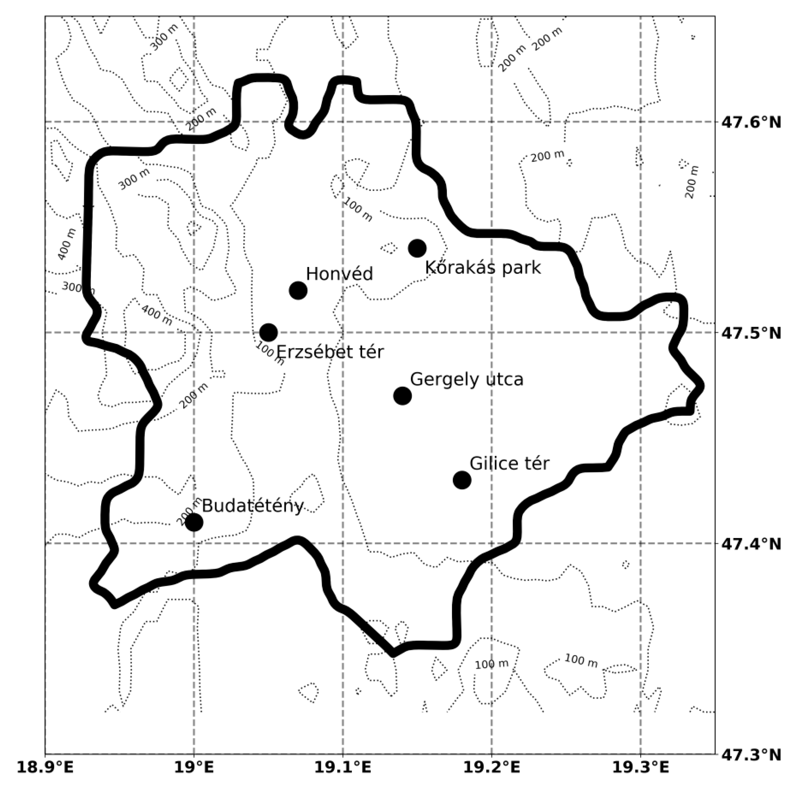
Figure 1. The administrative boundary of Budapest, the locations of monitoring sites and the CAMS output grid. Topography contours are drawn based on the GLOBE 1 km digital elevation model [46].
Atmosphere 11 00669 g001
Figure 2. Twenty-four-hour moving average PM2.5 measurements (black) at three urban monitoring sites compared with the CAMS ensemble median (red) and the fused prediction (blue). Bias-corrected CAMS ensemble and fusion of bias-corrected individual models are shown with points. The World Health Organization (WHO) guideline 25 µg/m3 is marked with a red line.
Atmosphere 11 00669 g002
Figure 3. Time series of daily root mean square error (RMSE) values between available hourly PM2.5 measurements and corresponding CAMS model predictions. RMSE of the fused prediction is marked with a black line. Gray bands indicate the polluted episodes.
Atmosphere 11 00669 g003
Figure 4. Comparison statistics between hourly PM2.5 observations in Budapest; the individual CAMS model predictions, the CAMS ensemble median, the 24-h persistence and the fusion of the models. Red bars indicate results obtained after a 10-day time-dependent additive bias-correction. The left column presents results for the entire 2018–2019 heating season, the center column for polluted episodes, and the right column for pattern shift days.
Atmosphere 11 00669 g004
Figure 5. Time series of fitted model weights. The PM2.5 concentration time series at one of the monitoring sites is presented for reference at the bottom of the figure. The horizontal axis is shared among all graphs.
Atmosphere 11 00669 g005
Table 1. Hourly PM2.5 data availability of monitoring stations and Copernicus Atmospheric Monitoring Service (CAMS) models in Budapest in the heating season 15 October 2018–15 April 2019.
StationLocationData AvailabilityMean ConcentrationNumber of Values Above 25 µg/m3
Budatétény47.41 N 19.00 E4327/4392 120 µg/m31157
Erzsébet tér47.50 N 19.05 E1871/4392 221 µg/m3621
Gergely utca47.47 N 19.14 E4367/439221 µg/m31333
Gilice tér47.43 N 19.18 E3120/4392 321 µg/m31050
Honvéd47.52 N 19.07 E4376/439219 µg/m31253
Kőrakás park47.54 N 19.15 E4389/439215 µg/m3749
ModelAreaData AvailabilityMean ConcentrationNumber of Values Above 25 µg/m3
CHIMERE47.45–47.55 N 19.05–19.15 E 4 4392/439215 µg/m3535
EMEP4368/439218 µg/m3951
EURAD4392/439216 µg/m3809
LOTOS-EUROS4392/439213 µg/m3285
MATCH4392/439212 µg/m3345
MOCAGE4392/439213 µg/m3461
SILAM4392/439224 µg/m31621
ENSEMBLE4392/439214 µg/m3523
1 Observations at Budatétény are missing until 17 October 2018. Data availability between 18 October 2018 and 15 April 2019 is 4317/4320. 2 PM2.5 observations at Erzsébet tér have ceased as of 2019. Data availability between 15 October and 31 December 2018 is 1871/1872. 3 Observations at Gilice tér are missing for March and April 2019. Data availability between 15 October 2018 and 26 February 2019 is 3105/3240 (96%). 4 Values from four CAMS model grid-points (47.45 N 19.05 E, 47.45 N 19.15 E, 47.55 N 19.05 E, 47.55 N 19.15 E) were used. The table shows the availability at all, the mean of all, and the exceedance at all four grid-points, respectively.
Table 2. Selected temporal subsets within the heating season 15 October 2018–15 April 2019.
Episode DaysPattern Shift Days
15–20 Oct 201821 Oct 2018
27 Oct 2018
1–3 Nov 20181 Nov 2018
5–13 Nov 201814 Nov 2018
1–4 Dec 20181 Dec 2018
6–8 Dec 20189 Dec 2018
13 Dec 2018
16–22 Dec 201816 Dec 2018; 23 Dec 2018
7–10 Jan 20197 Jan 2019; 11 Jan 2019
21–25 Jan 201921 Jan 2019
27 Jan–1 Feb 20192 Feb 2019
6–10 Feb 20196 Feb 2019; 11 Feb 2019
15–19 Feb 201915 Feb 2019; 20 Feb 2019
25 Feb 2019
22 Mar 2019
24 Mar 2019

