Evaluation of Hurricane Harvey (2017) Rainfall in Deterministic and Probabilistic HWRF Forecasts

Abstract

Rainfall forecast performance was evaluated for the first time for the Hurricane Weather Research and Forecasting (HWRF) model. This study focused on HWRF performance in predicting rainfall from Hurricane Harvey in 2017. In particular, two configurations of the 2017 version of HWRF were investigated: a deterministic version of the Basin-scale HWRF (HB17) and an ensemble version of the operational HWRF (H17E). This study found that HB17 generated reasonable rainfall patterns and rain-rate distributions for Hurricane Harvey, in part due to accurate track forecasts. However, the estimated rain rates near the storm center (within 50 km) were slightly overestimated. In the rainband region (150 to 300 km), HB17 reproduced heavy rain rates and underestimated light rain rates. The accumulated rainfall pattern successfully captured Harvey’s intense outer rainband with adequate spatial displacement. In addition, the performance of H17E on probabilistic rainfall has shown that the ensemble forecasts can potentially increase the accuracy of the predicted locations for extreme rainfall. Moreover, the study also indicated the importance of high-resolution dynamical models for rainfall predictions. Although statistical models can generate the overall rainfall patterns along a track, extreme rainfall events produced from outer rainbands can only be forecasted by numerical models, such as HWRF. Accordingly, the HWRF models have the capability of simulating reasonable quantitative precipitation forecasts and providing essential rainfall guidance in order to further reduce loss of life and cost to the economy.

1. Introduction

Rainfall is a major hazard associated with a landfalling tropical cyclone (TC). In fact, water causes more TC-related deaths than winds. Overall, about ninety percent of fatalities are caused by water-related events, and rainfall-induced events, such as freshwater flooding and mudslides, contributed about a quarter of fatalities [1]. Although TC rainfall prediction is important, it remains a major forecast challenge. Earlier studies based on statistical models (e.g., [2,3,4]) have illustrated that accurate TC track predictions should lead to an improvement of rainfall prediction in landfalling TCs. Moreover, several other factors such as storm speed, storm structure, topography, and environmental moisture can also influence TC precipitation.

In 2017, Hurricane Harvey made landfall in Texas and Louisiana in the U.S. as a category four hurricane on the Saffir–Simpson Hurricane Wind Scale [5], causing extreme accumulated rainfall of greater than three feet in a large area over five days, with a maximum of 60.58 inches in Jefferson, Texas [6]. Hurricane Harvey reached major hurricane status at 1800 UTC 25 August and made landfall at 0300 UTC 26 August. Harvey was the first major hurricane to make landfall in the U.S. since 2005. After landfall, Hurricane Harvey meandered over southeastern Texas for more than 60 h until moving back over the Gulf of Mexico at 1800 UTC 28 August, delivering prolonged heavy precipitation to the region. Even after Harvey moved offshore, it continued to produce heavy rainfall over Texas and Louisiana until 30 August, when it made a second landfall in Louisiana and finally dissipated. The disastrous rainfall from Harvey’s outer rainbands occurred in the nearly constant onshore flow to the northeast of Harvey’s center, with the Gulf of Mexico continuously supplying moisture to support heavy precipitation [6]. According to the National Oceanic and Atmospheric Administration (NOAA), Hurricane Harvey caused more than 68 direct deaths and about 125 billion dollars in economic loss, making it the second-costliest TC after Hurricane Katrina [7]. Hurricane Harvey’s primary threat was freshwater floods in highly populated regions induced by constant heavy rainfall. Houston’s urbanization may also have exaggerated flood response and increased accumulated rainfall [8,9], and anthropogenic activities may shorten return periods and increase the frequency of such an event [10,11]. Moreover, a slow-moving TC is likely to produce more rainfall than a fast-moving TC. Due to Harvey’s storm speed and constant moisture supplies, this flooding hazard extended well inland, continued to affect an area after landfall, and caused catastrophic destruction. Therefore, an accurate rainfall prediction is critical for disaster management for reducing loss of life and cost to the economy.

Although TC rainfall can cause significant damage or loss of life, it is also an essential source of freshwater in many regions globally [12]. Hence, studies that evaluate and improve current numerical quantitative precipitation forecasts (QPFs) are indispensable. Numerous studies focused on QPF validation techniques to evaluate the utility of rainfall forecasts. Initially, the threat score (TS), which is also known as critical success index (CSI) [13,14], was utilized to validate QPF (e.g., [15]). Nowadays, the equitable threat score (ETS) [16] is more commonly used as it accounts for random model predictions (e.g., [17,18,19]). Ebert et al. [20] used bias score and ETS to verify numerical models, including the NOAA National Centers for Environmental Prediction (NCEP) Eta model and the European Centre for Medium Range Forecasts (ECMWF) Integrated Forecasting System (IFS), against rain gauge data in regions of the United States, Germany, and Australia.

Besides various scoring methods, Lonfat et al. [2] studied the National Aeronautics and Space Administration (NASA) Tropical Rainfall Measuring Mission (TRMM) data and provided guidance on the TC rainfall climatology through evaluating rain profiles with rain rate probability distribution functions (PDFs) and contoured frequency by radial distance (CFRD), which represents PDFs as a function of the radius from the storm center. This study also suggested the use of a decibel rain rate (dBR) scale to produce PDF and CFRD diagrams as rain rate is nearly log-normally distributed [2]. Furthermore, Marchok et al. [4] developed a standard scheme for validating QPF in landfalling TCs to examine NCEP operational models, and this scheme includes three components: the pattern matching ability, mean rainfall and volume matching skill, and the ability to capture extreme amounts. Moreover, a numerical model is typically considered practical and beneficial only when it outperforms a statistical model. The Rainfall Climatology and Persistence (R-CLIPER) model is commonly used as a standard baseline of statistical TC rainfall predictions [4,21]. Lonfat et al. [3] developed another version of R-CLIPER, called Parametric Hurricane Rainfall Model (PHRaM), to take account of shear and topography effects.

With the aid of these rainfall evaluating approaches, several challenges of numerical model prediction for rainfall have been addressed. Tuleya et al. [21] pointed out that rainfall performance was highly dependent on both storm intensity and track from the evaluation of the Geophysical Fluid Dynamics Laboratory (GFDL) model performance. Marchok et al. [4] also emphasized the importance of track forecasts in order to obtain a better rainfall prediction, noting that track bias is possibly caused by physical parameterizations or initialization schemes. Moreover, model resolution may also be key to capture improved storm structure or a more realistic storm intensity. The study from Ebert et al. [20] stated that models may experience more difficulties in predicting convective rainfall in summer than synoptic-scale rainfall in winter in the U.S. On the other hand, Weisman et al. [22] suggested that 4-km resolution is sufficient for simulating mesoscale cloud systems, and cloud parameterization is not required for such a high-resolution model. Roberts and Lean [23] examined the impact of resolution on rainfall prediction of the United Kingdom Met Office Unified Model. Their study addressed that a higher-resolution model can improve the prediction for heavier and more localized rain [23]. Wu et al. [24] verified the NASA-unified Weather Research and Forecasting (NU-WRF) [25] model to investigate the land surface impacts on rainfall; the study also highlighted 3-km NU-WRF has higher accuracy on rainfall predictability than 9-km NU-WRF. Accordingly, a high-resolution forecast model with demonstrated track and intensity prediction skills may potentially lead to more reliable and sensible rainfall estimations.

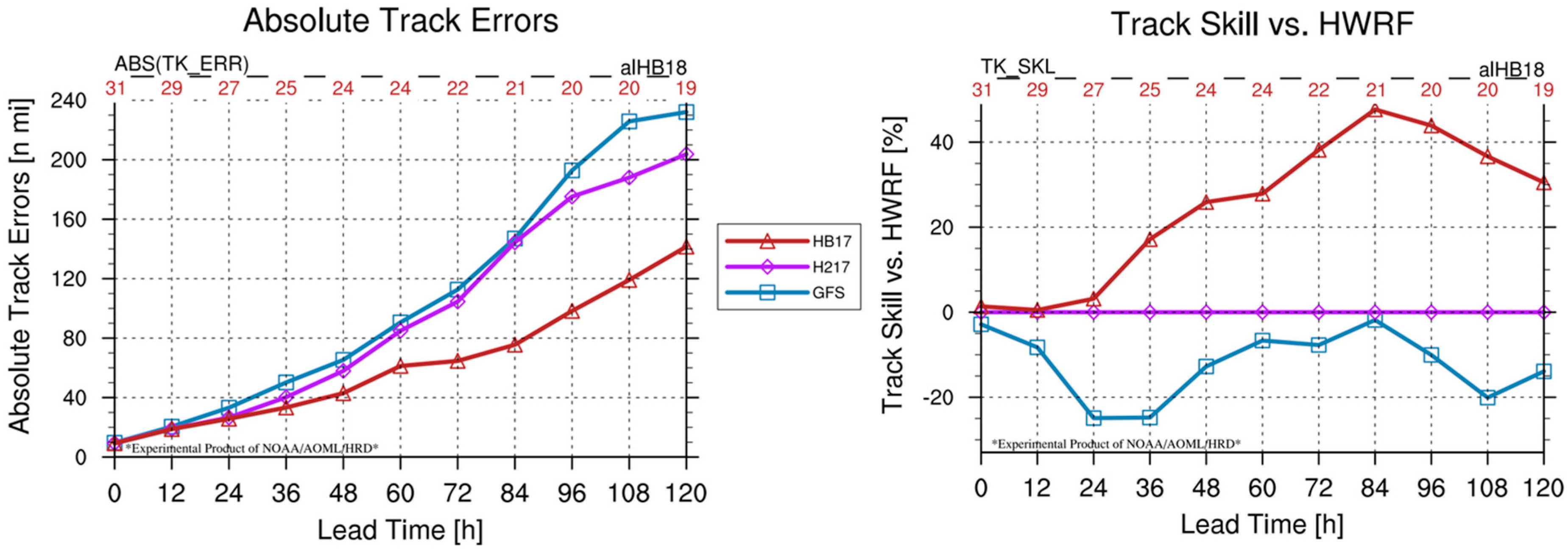
The Hurricane Weather Research and Forecasting (HWRF) modeling system has been critical to the improvement of TC predictions at NOAA and across the globe. The HWRF model is a regional numerical weather prediction (NWP) model that specializes in TC guidance [26,27,28,29]. For the last decade, the Hurricane Forecast Improvement Program (HFIP) [30] has supported improvements to TC track and intensity predictions in HWRF, and, recently, the focus of HFIP has expanded to TC hazards, including rainfall. This study is the first to examine hurricane rainfall predictability of a high-resolution HWRF system following the rainfall evaluation guidance from the studies mentioned above. The NCEP Environmental Modeling Center (EMC) implemented HWRF with high nested resolutions for real-time operation [31]. Apart from a deterministic forecast, HWRF has also implemented an ensemble prediction system (EPS) to provide probabilistic predictions for better forecast guidance. This HWRF-based EPS takes account of initial and boundary condition perturbations and model physics perturbations [32,33]. On the other hand, with the support of HFIP and in collaboration with EMC, the National Weather Service (NWS), and the Developmental Testbed Center (DTC), the Hurricane Research Division (HRD) of the NOAA Atlantic Oceanographic and Meteorological Laboratory (AOML) developed and maintained an experimental “Basin-scale HWRF” model (HWRF-B) [34,35,36]. HWRF-B produced low track errors in 2017 compared with other NOAA models. Due to the high dependence of precipitation on TC track, HWRF-B is leveraged as a rainfall research tool to evaluate the precipitation performance for Hurricane Harvey. In addition, HWRF EPS is also being investigated in this project to explore the potential of probabilistic precipitation forecasting. The ultimate goals of this project are to evaluate TC rainfall performance in NWP and to create new probabilistic rainfall guidance for TC landfalls. Section 2 describes the methodology of this project, including the models, datasets, and forecasts of interest. Section 3 presents the results of the rainfall performance in HWRF-B forecasts and introduces NWP-based probabilistic guidance. Section 4 discusses the overall results and the findings of this case study, and conclusions are provided in Section 5.

2. Materials and Methods

2.1. HWRF Models

In this study, two versions of HWRF-based models are investigated for their rainfall predictability: the 2017 version of HWRF-B (HB17) [36] and HWRF EPS of the same year (H17E). HWRF-B is an experimental non-hydrostatic numerical model maintained by NOAA/AOML/HRD. This model was originally developed in 2012; is updated annually based on the operational HWRF and has been operating as an HFIP real-time demonstration project since 2013. Different from the operational version, HWRF-B has a fixed outermost domain covering both the North Atlantic basin and Eastern North Pacific basin. This gives the advantage of configuring several high-resolution movable multi-level nests (MMLN) [35] for simulating storms simultaneously within the same integration. In 2017, HWRF updated the model resolution to 18/6/2 km for each domain, respectively, to increase the accuracy of TC simulations. As discussed, rainfall forecasts have high dependence on track forecasts. Figure 1 shows that HB17 produced lower track forecast errors than the operational HWRF (H217) [29] and the Global Forecast System (GFS), making it ideal to study precipitation forecasts. The HB17 mean absolute track error was about 70 n mi (130 km) at 72 h and 160 n mi (300 km) at 120 h. HB17 track forecasts were about 30% more accurate than H217 forecasts at 72 h and later lead times. With such skillful track forecasts, HB17’s prediction of rain accumulation was analyzed against observational datasets. The other model examined is H17E, which considers uncertainties induced by initial conditions (data assimilation), boundary conditions (for regional models like HWRF), or model physics or dynamics (such as convective clouds, large scale environment, and multi-scale interactions among sub-grid scales) [32,33]. The EPS has the same nested configuration and resolution as the H217 model and provides 21 ensemble members for probabilistic predictions. This study aims to evaluate the potential of probabilistic rainfall predictions of H17E.

2.2. Baselines

NCEP generates regional multi-sensor quantitative precipitation estimates (QPE) with quality controls from 12 River Forecast Centers (RFCs) and archives them as Stage IV (ST4) products. The multi-sensor Stage IV QPEs combine approximately 140 Weather Surveillance Radars—1988 Doppler (WSR-88D) with hourly precipitation reports from the 1450 Automated Surface Observing Stations (ASOS) sites and about 5500 Hydro-meteorological Automated Data System (HADS) automated gauge reports [37]. The radar estimates are collected within a 10-min window at the top of the hour and used a simple inverse-distance weighted average for overlapping areas between adjacent radars. Fulton et al. [38] documented the details of radar estimate merging and bias removal algorithms. Stage IV products are in the National Weather Prediction Hydrologic Rainfall Analysis Project (HRAP) grid with a 4-km spatial resolution. The HRAP grid is an 1160 × 880 polar stereographic projection covering the Contiguous United States. Nelson et al. [39] found that the Stage IV estimates show an overall general bias of underestimating rain rates. However, the heavier rain rates, such as in TCs, were shown to have lower fractional standard errors than lighter rain rates. Our study focuses on the coastal area of the Gulf of Mexico, which was shown to have better rain rate estimates in the fall season (September to November) with reasonable bias (varying between 0.83 and 1.26) and high general correlations (0.88 to 0.93). Thus, the Stage IV QPEs may provide the best rainfall analysis for evaluating the model TC rainfall in this study.

Another observational data source is the Integrated Multi-satellite Retrievals for NASA Global Precipitation Measurement (IMERG). IMERG combines all available satellite microwave precipitation estimates from microwave-calibrated infrared satellite estimates, and rain gauge data from about 16,000 sites globally [40]. IMERG has provided QPEs half-hourly in 0.1-degree resolution since 1998, and each estimate has three versions: Early, Late, and Final. In this study, we chose the Final version as it is a reanalysis product based on multi-satellite estimates from Early and Late runs (real-time runs) adjusted by monthly rain gauge data and climatological calibration coefficients. Additional information about the algorithms can be found in Huffman et al. [40]’s Algorithm Theoretical Basis Document. Studies noted that IMERG data tends to underestimate intensive rainfall events in warm seasons due to misinterpretation from IMERG microwave sources [41,42]. Moreover, IMERG dataset has a coarser resolution compared to Stage IV, and QPE over the ocean is only from satellite data without any direct ground-based gauge or radar adjustments. Nevertheless, IMERG is currently the best resource to estimate precipitation over the ocean. Stage IV, a ground-based rainfall dataset with a 4-km resolution, may provide more rainfall distribution details than IMERG. Due to different strengths of the two QPE datasets, we assumed that the Stage IV QPE as “truth” over land and the IMERG over the ocean in this study.

The R-CLIPER (RCLP) model was developed for validating the rainfall prediction performance of NWP models. This statistical model was first established based on hourly rain gauge data in the U.S. from 1984 to 2000, including 120 landfalling storms [43]. The rain rate in the R-CLIPER model is a function of the time after landfall and the distance from a storm center, and it is partitioned between tropical storms and hurricanes. R-CLIPER was updated to use the Lonfat et al. [2] TC rainfall climatology that included more than 400 TCs globally allowing the rain rate to be partitioned as a function of storm intensity, with wind speeds at: tropical storm strength; hurricane strength (category 1–2 on Saffir–Simpson wind scale); and major hurricane strength (category 3–5) from TRMM. Tuleya et al. [21] presented a comparison between the two approaches of QPEs. These methods both showed similar azimuthal mean rain-rate profiles on tropical storm cases. TRMM’s hurricane-strength rain-rate profile matched the gauge’s “hurricane” profile. However, the TRMM data was able to provide rain-rate estimations for major hurricanes, while the gauge data could not, and was not restricted to be over land. Therefore, our study chose to validate the TRMM version of R-CLIPER.

2.3. Evaluation

One way to evaluate model performance is to compare with observational data, such as radar, rain gauge, or satellite data. Evaluating against a statistical model can also show whether a model is practical for operations. This study investigates HWRF-based models against Stage IV radar products, IMERG, and R-CLIPER. In order to capture the landfall and subsequent stall for heavy rainfall simulation, we evaluated these forecast cycles from HB17: 0000 UTC 24 August 2017, 1800 UTC 24 August 2017, and 0000 UTC 25 August 2017. These cycles are about 24 to 48 h before landfall, which can provide essential guidance for hurricane warnings. For H17E, as the cost of running the ensemble experiment for the real-time forecasts is not yet realistic, we only selected one cycle here for exploring the potential benefits of utilizing EPS for hurricane rainfall guidance. The selected cycle from H17E is 0000 UTC 25 August 2017, which provides us the probabilistic rainfall prediction at least 24 h before landfall (Figure 2). Due to the limited WSR-88D radar coverage range, the evaluation lead time for 0000 UTC 24 August 2017 cycle is from forecast hour 15 to 126. Forecast hour 15 was the first to capture at least half of the storm structure from Stage IV. For the other two selected cycles, the entire forecast lead time (0–126 h) was examined.

This study follows the evaluation procedures from both Lonfat et al. [2] and Marchok et al. [4] to examine the model rainfall performance. We first evaluate HB17’s ability to capture rainfall patterns by comparing spatial accumulated rainfall distributions, CSI, and bias score against the observational data and R-CLIPER. The spatial rainfall distribution is from the HB17 5-km swath data, which was properly interpolated by HWRF from the original nested output. As the data is on a pre-segmented storm-track domain instead of the entire model domain, defining model random correct forecasts for computing ETS becomes trivial. Therefore, we measure the rainfall pattern-matching skills with CSI and bias scores. Then, we further investigate precipitation structure relative to the storm center for assessing azimuthal rain-rate distribution with the model 2-km-resolution output data. Additionally, the performance of probabilistic rainfall prediction from H17E is generated to understand how the rainfall patterns adjust when considering 21 possible situations.

3. Results

3.1. Pattern Analysis

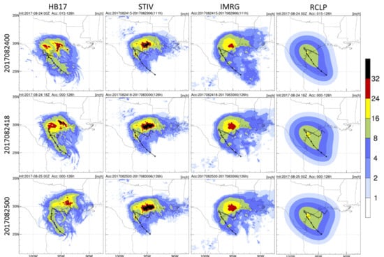
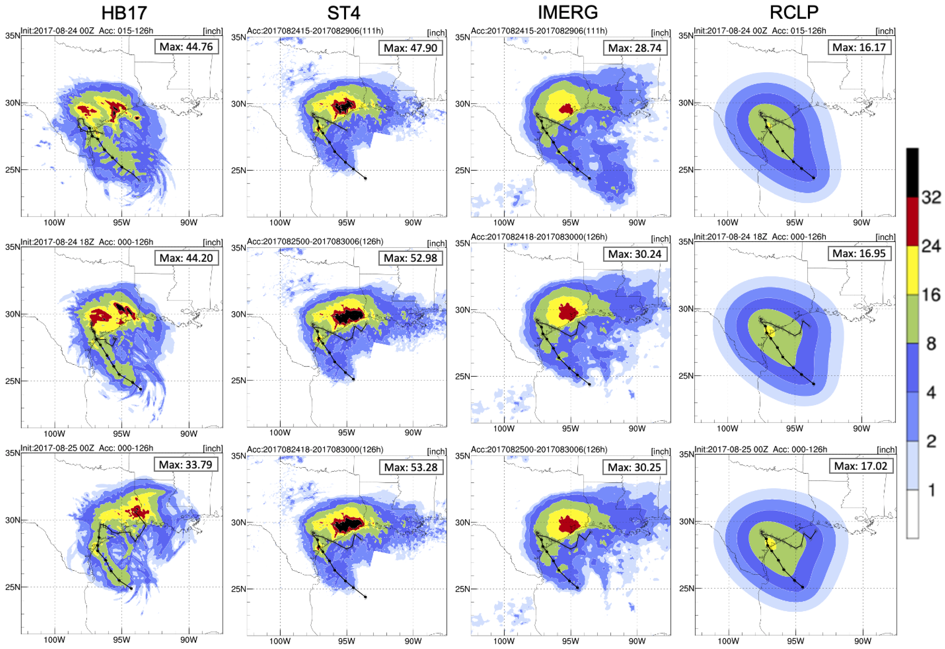
The precipitation pattern analysis is a tool used to examine model performance for accumulated rainfall distribution. Figure 3 shows total precipitation accumulated during Hurricane Harvey for the three deterministic HB17 forecasts corresponding to periods of 111, 126, and 126 h. Rainfall totals from Stage IV, IMERG, and R-CLIPER were calculated for the same periods. Typically, TC rainfall patterns show the heaviest accumulated precipitation in the eyewall region where the strongest convection occurs. Hurricane Harvey was unusual in that it produced significant rainfall in its outer rainbands, especially those remaining offshore. Observations indicate that the greatest rainfall accumulation occurred over the Houston region whereas the eye had limited direct impact. In addition, IMERG shows rainfall over the ocean was not significantly strong along the track. Stage IV and IMERG show similar rainfall distributions over land, yet Stage IV presents more intense and a broader rainfall accumulation maximum over the Houston area to the Texas–Louisiana border. Stage IV captured 47 to 53 inches of extreme accumulated rainfall, which is about 1.7 times higher than the maximum value from IMERG. The disagreement between two observational data is possibly related to the data resolution, data collection, or calibration. Even though both data were corrected by rain gauges, Stage IV, with the higher resolution and the ground-based measurement, can better represent extreme rainfall values.

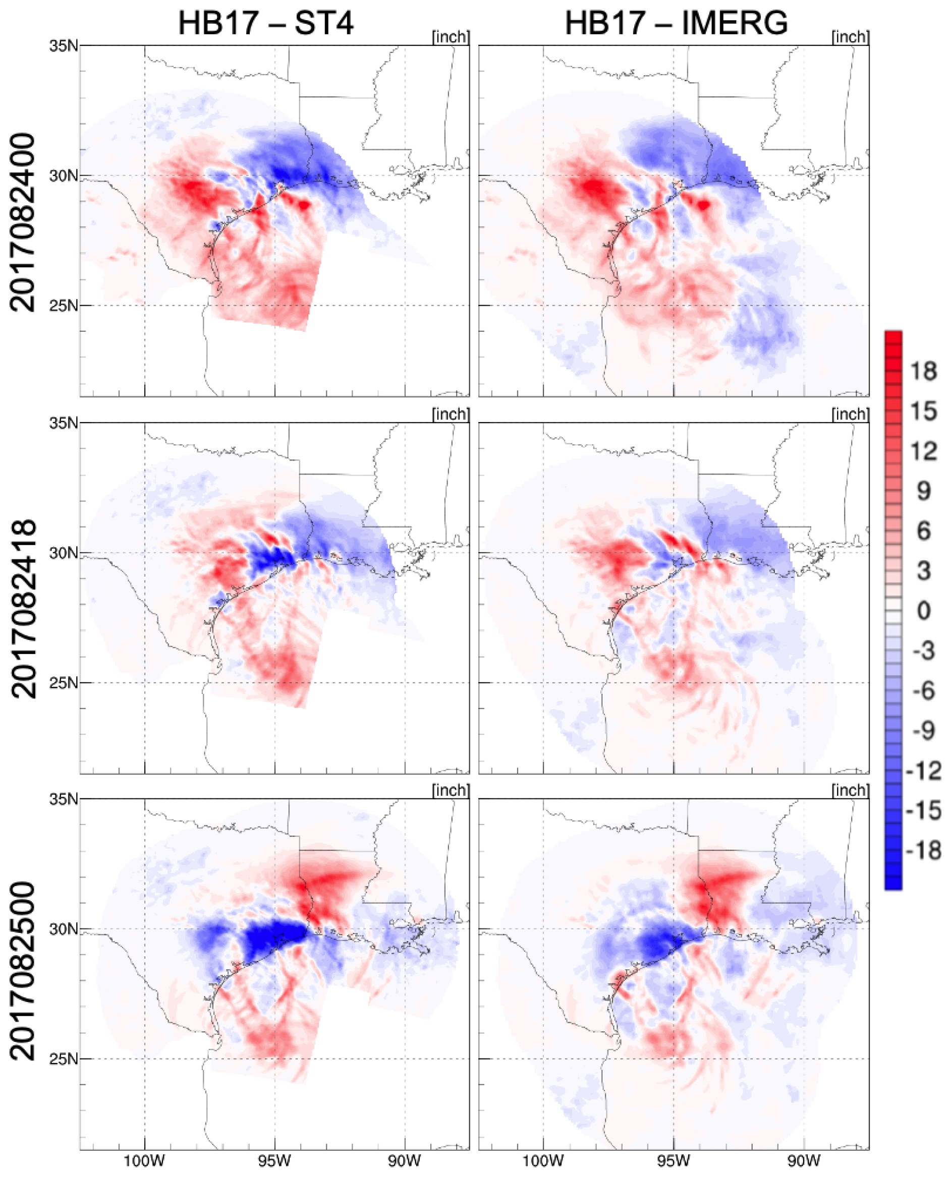
The climatological model, R-CLIPER, only shows a main rainfall accumulation pattern along the track without the heavy rainfall accumulation over Houston. The result indicates the heaviest accumulation was at the landfall location; also, the overall rainfall accumulation on land was below 17 inches, which is much lower than the Stage IV accumulation. Compared to R-CLIPER, HB17’s pattern is more similar to the Stage IV and IMERG estimates. In the first two selected cycles, HB17 predicted a large rainfall accumulation occurring not only over Houston, but also over Austin and San Antonio. This second peak-rainfall accumulation was not present in the 0000 UTC 25 August 2017 cycle. The peak value of Houston’s heavy rainfall accumulation dropped from 44 to 33 inches, and the peak center moved towards the east as the second landfall occurred in Louisiana in this cycle. HB17 also predicted a clear strong rainfall accumulation pattern along its track over the ocean as expected. The general rainfall pattern from HB17 appears much more realistic than the one from R-CLIPER in terms of the prediction of the peak rainfall location and the amount of rainfall. The comparison between the HB17 model prediction and Stage IV and IMERG is shown in Figure 4. The dipole patterns suggest that the rainfall amount is realistic, but the location shifted. In the first two selected cycles, HB17 overestimated rainfall on the west side of the Texas coastal region and underestimated rainfall on the east side. The amplitudes of the contradictory estimations are comparable. However, in the last cycle, the overestimation pattern shifted from the coastal region of Texas to Louisiana. The shifted dipole pattern indicates that the peak rainfall location was too far to the east, and HB17 still missed the rainfall over the east coastal region of Texas. Moreover, over the Gulf of Mexico, the rainfall was mostly overestimated.

The spatial rainfall patterns show that the HB17 rainfall prediction is significantly better than R-CLIPER. Hurricane Harvey’s strong outer rainband violates the simple symmetric rainfall model in R-CLIPER. Also, the R-CLIPER’s rainfall estimates, while a function of intensity, use the mean rain rate for each intensity class preventing it from correctly capturing a realistic rainfall pattern for this storm. On the other hand, HB17 has the capability to predict realistic rainfall patterns when the peak rainfall falls in the outer rainband region, yet the extreme accumulated rainfall values were missed. Moreover, the extreme values indicate that IMERG has difficulty representing extreme rainfall overland. As IMERG only provides the information on the rainfall distribution over the ocean, the later part of this study will focus on the evaluation of the HWRF models against Stage IV and R-CLIPER.

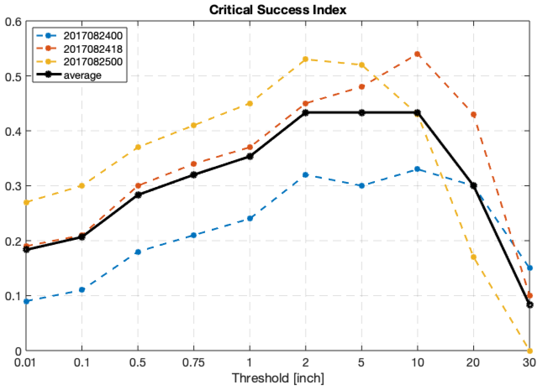
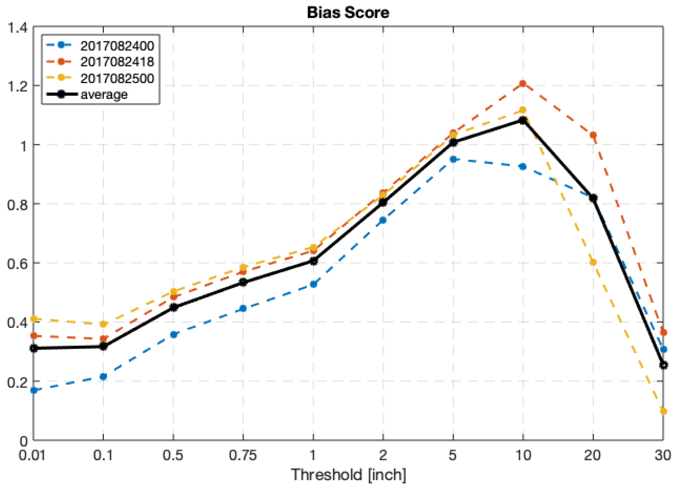
The CSI in Figure 5 shows HB17 made better predictions in the later cycles. The results from 0000 UTC 25 August gave the best simulations on rain rates below 5 inches, and 1800 UTC 24 August presented the best heavy rainfall simulations (above 10 inches). On average, HB17 is more skillful at predicting accumulated rainfall between 2 to 10 inches than predicting light or heavy rainfall amounts. The bias scores in Figure 6 present that the model has overall underestimation of observed rainfall amounts, especially for both light (below 1 inch) and extreme (30 inches) accumulated rainfall. Both CSI and bias scores indicate that HB17 predicted accumulated rainfall between 1 to 10 inches better than other thresholds. The missing light rain over eastern Texas may be the reason for the low bias score and CSI of the light rainfall thresholds; imperfect extreme rainfall values and location are possibly responsible for the low scores of the heavy rainfall thresholds.

In this analysis, we found that, with accurate track prediction, HB17 has the capability of predicting a considerably accurate rainfall pattern. Even though the peak rainfall accumulation from HB17 was not correctly predicted, the general amount of rainfall was convincing and could have been useful forecast guidance. The underestimation of extreme values of rainfall may be resolved by enhancing the model physics or parameterizations, and spatial displacement of extreme rainfall may be further improved by the probabilistic rainfall predictions in order to provide a more sensible guidance for forecasting centers.

3.2. Azimuthal Analyses

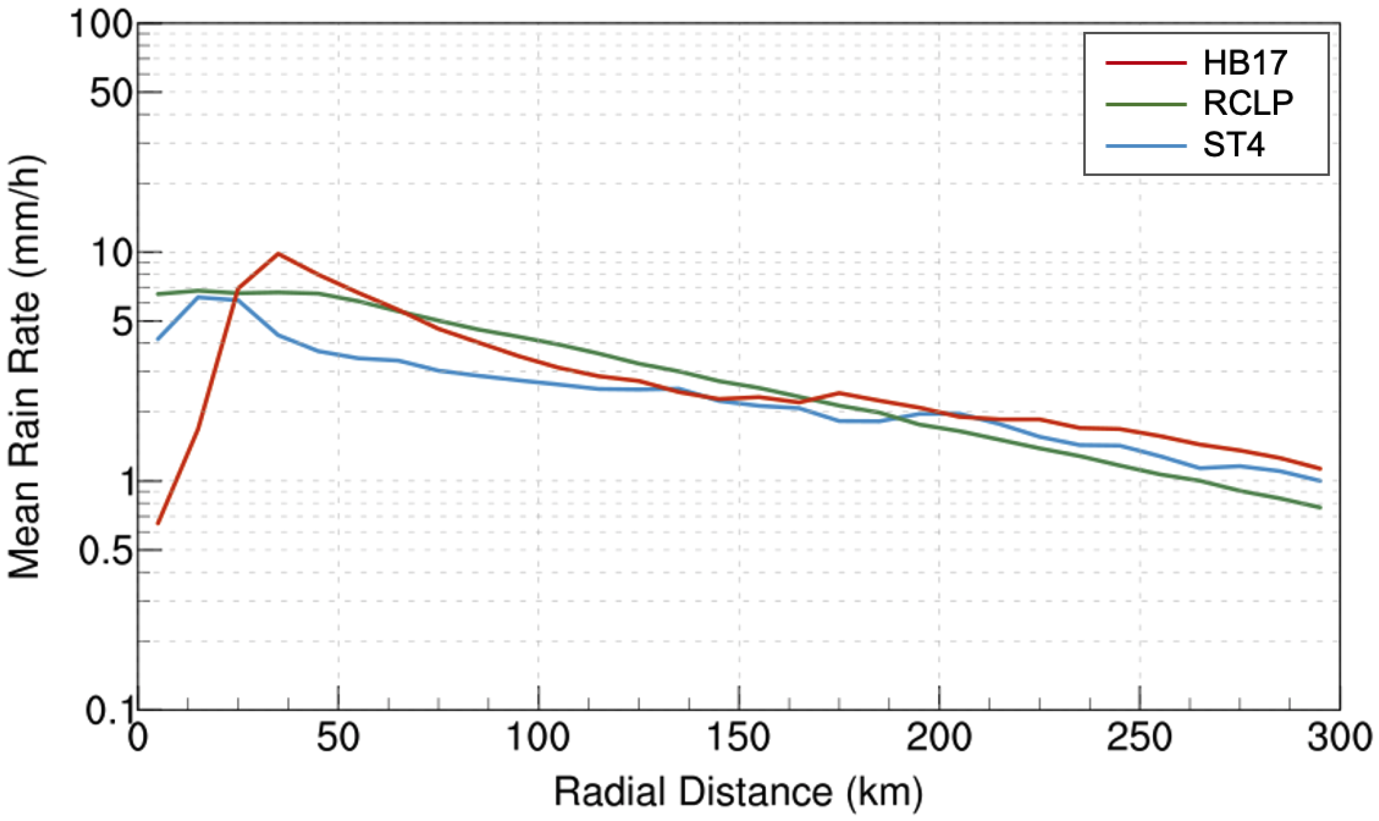
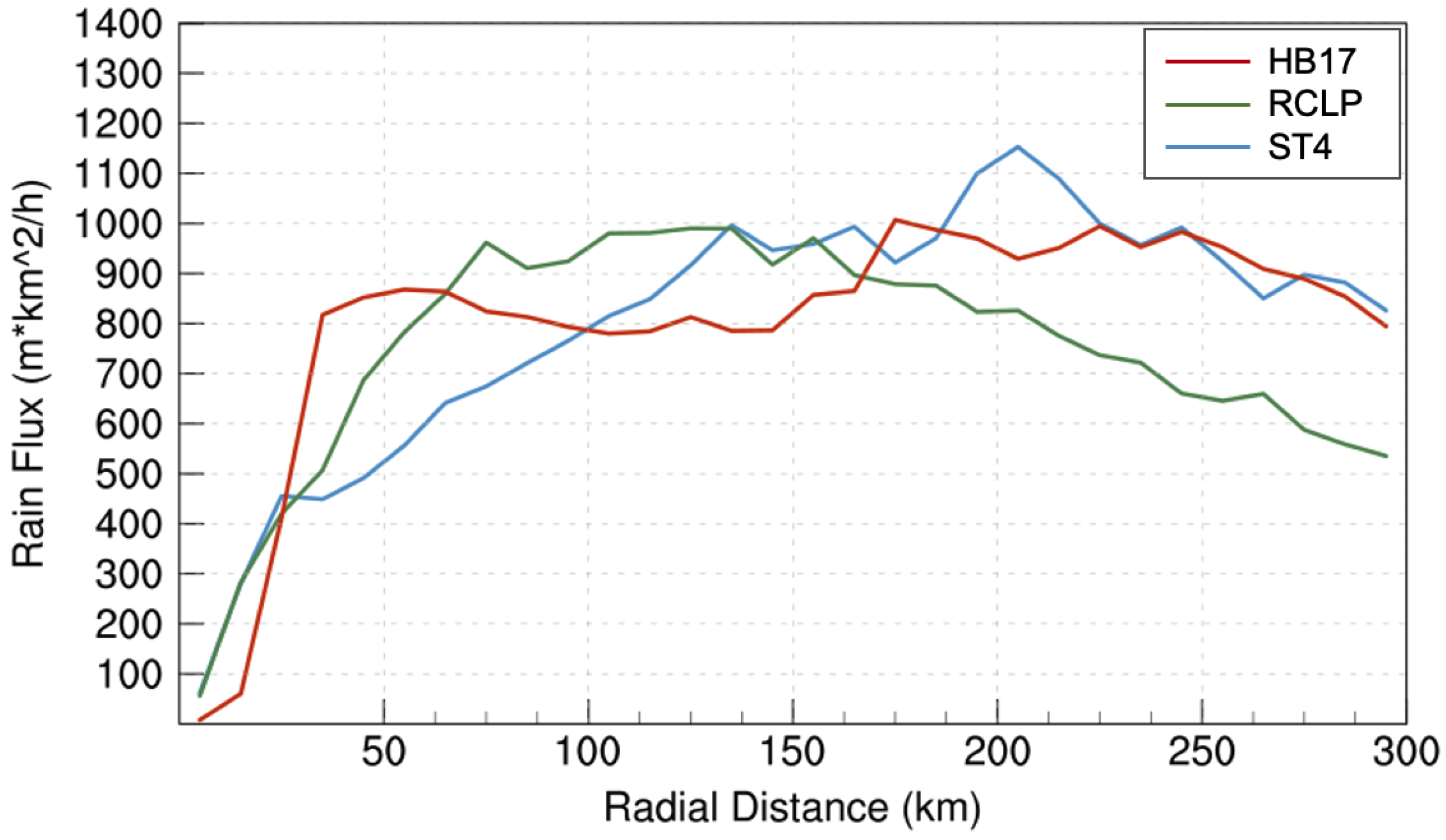
The azimuthal analysis statistically examines precipitation structures from the center to the outer rainband to assess the rain rate performance of peaks, trends, and distributions. In this study, rain rates are plotted on a logarithmic scale as rain is log normally distributed. Rain-rate values are averaged within each 10 km radius interval from 0 to 300 km. Figure 7 shows radial distribution of averaged rain rates. R-CLIPER (green) predicts a slightly steeper slope than the other datasets. The peak averaged rain rate remains at 7 mm h${}^{-1}$ in the core, within 50 km, and the value decreases to 1 mm h${}^{-1}$ in the outer rainband area (100 to 300 km). HB17’s prediction (red) is very close to observational values (blue and purple), especially in the outer rainband. However, in the core region, HB17’s prediction does not match with observational data. Stage IV captures small changes in rain rates varying from 3 to 6 mm h${}^{-1}$, and HB17’s value changes from below 1 mm h${}^{-1}$ at the storm center to a peak of 10 mm h${}^{-1}$ at 40 km from the center. Due to the high resolution (2 km), HB17 is able to present a clearer eye structure compared to the others. The Stage IV estimates also capture an eyewall-like structure with the 4-km resolution. Low-resolution data tend to smooth out extreme values, which are able to be preserved in a high-resolution dataset.

However, both resolution and overestimation can contribute to this peak value, so it is necessary to consider the impact of resolution differences between datasets. Rain flux, shown in Figure 8, is a function of rain rate and resolution.

$$RainFlux=RainRate\ast {\left(Resolution\right)}^2.$$

(1)

Rain flux indicates total amounts of rain within each 10 km annulus around the storm. The rain flux of HB17 is consistent with the observational rain flux from 150 to 300 km, but the amount within 40 to 50 km is almost twice as much as observed. R-CLIPER overestimates the rain flux from the center to 120 km, but it decreases rapidly from 150 to 300 km.

In these radial distribution analyses, HB17 shows skill in producing reasonable rain rates and rain flux for the outer rainband region. R-CLIPER did not produce rain rates similar to Harvey’s rainband region. Similar to Stage IV, HB17 has the capability to produce a clear eyewall structure, but the rain rates in the eye are slightly overestimated.

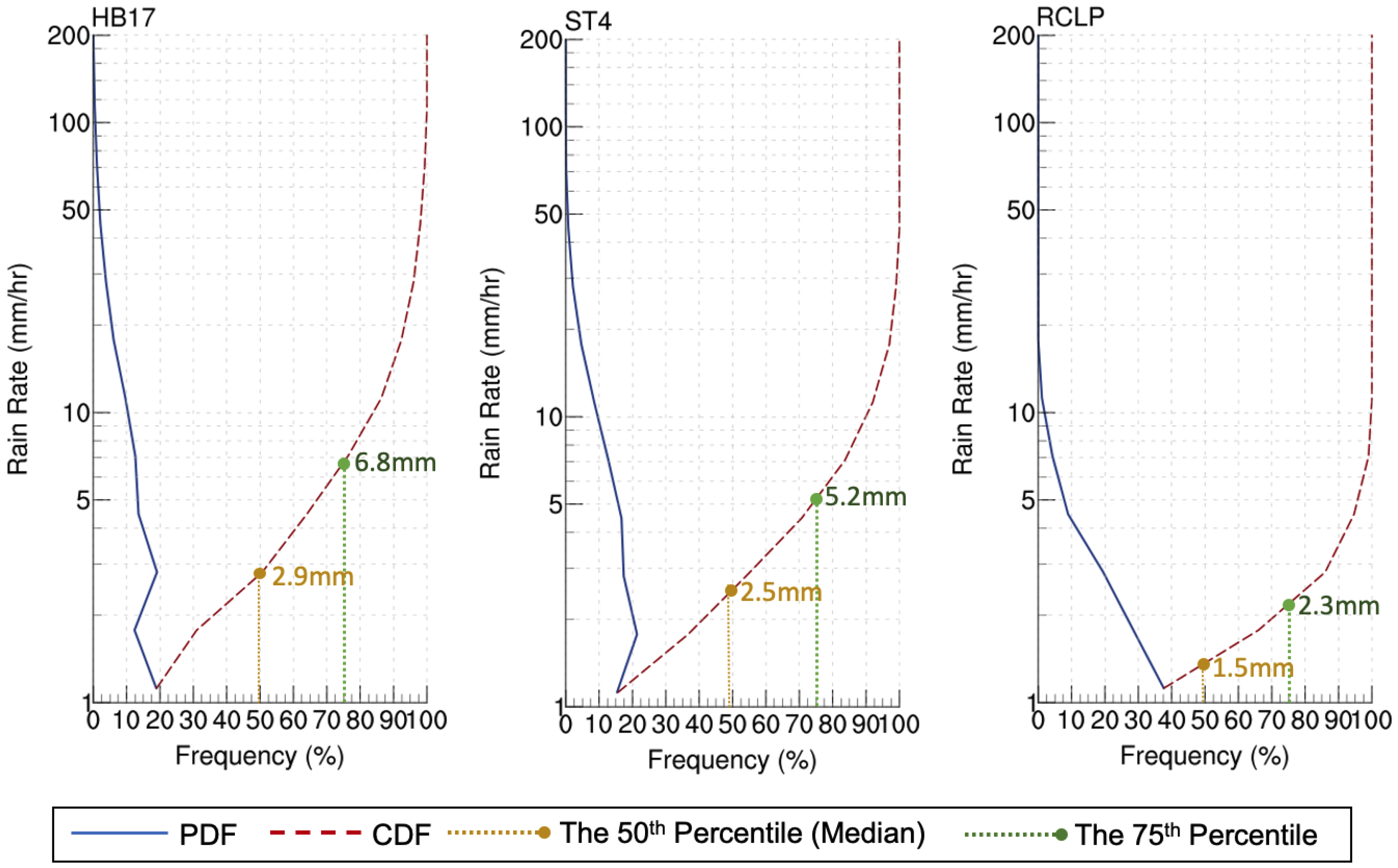
Probability distribution functions (PDFs) and cumulative distribution functions (CDFs) of rain rate (dBR) in Figure 9 shows the model light/heavy precipitation compared to the observations.

$$dBR=10\ast {log}_{10}\left(RainRate\right).$$

(2)

The PDF and the CDF are originally calculated over the rainfall range 0 dBR (1 mm h${}^{-1}$) to 27 dBR (500 mm h${}^{-1}$) in 14 steps, or 2 dBR intervals. Figure 9 only shows up to 200 mm h${}^{-1}$, and the results show that the median rainfall rate for HB17 (yellow dot) is 2.9 mm h${}^{-1}$, R-CLIPER is 1.5 mm h${}^{-1}$, and Stage IV is 2.5 mm h${}^{-1}$. Accordingly, HB17 produces reasonable amounts of both lighter and heavier rainfall, whereas R-CLIPER produces a significant amount of lighter rainfall, resulting in a low value of the median. On the other hand, HB17’s 75th percentile (green dot) is 6.8 mm h${}^{-1}$ while Stage IV is 5.2 mm h${}^{-1}$, suggesting that HB17 produces a greater proportion of extreme rainfall than the observational data. The PDF reveals similar information. R-CLIPER produces a significant amount of light rain (below 5 mm h${}^{-1}$) and rarely produces rainfall above 10 mm h${}^{-1}$. HB17’s PDF shows this model produces about 2% of rainfall above 50 mm h${}^{-1}$ and a very small amount of rainfall around 80–90 mm h${}^{-1}$. However, Stage IV captures less than 1% above 50 mm h${}^{-1}$. In general, HB17’s PDF profile is comparable to the one from Stage IV but 1% exceeds 100 mm h${}^{-1}$. The PDF and the CDF both suggest that HB17 generally produces a representative dBR/rain rate with a slightly higher frequency of extreme rainfall (>50 mm h${}^{-1}$). Compared to the results from HB17, R-CLIPER’s profiles are less representative because many light rain rates were generated.

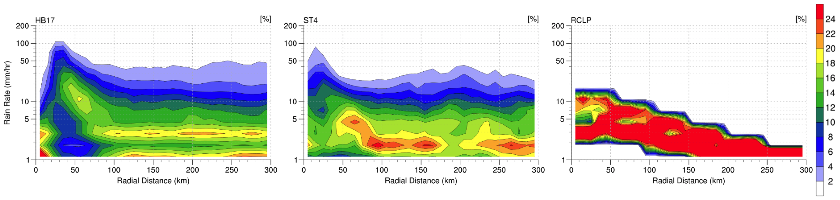
The CFRD plots are shown in Figure 10. These depict the PDFs within each 10 km annulus from 0 to 300 km. CFRD shows how the PDF varies from the center to the outer rainband region and helps locate where the overestimation of extreme rainfall (>50 mm h${}^{-1}$) happened. In Stage IV’s CFRD profile, lighter rain rates are the majority of the rainfall in the core region, but about 20% of rainfall is contributed by heavy rain rates (10–50 mm h${}^{-1}$). The trend of heavy rainfall also decreases with the distance from the eyewall and increases again around 150 to 250 km. The outer rainband as stated contributes to this increasing trend.

R-CLIPER’s CFRD shows rain rate gradually decreased from the center to the outer region. At the center, the rain rate mostly varies from 3 to 10 mm h${}^{-1}$. All rain rates are below 5 mm h${}^{-1}$ from 150 to 300 km. Due to R-CLIPER’s algorithm, the predicted rain rates are highly concentrated in a certain range for each 10-km interval. Unfortunately, compared to the observational dataset, R-CLIPER does not produce a realistic radial rain-rate frequency. In reality, light rain rate can exist in a strong convection area where heavy rainfall usually occurs. On the other hand, heavy rain rates can be observed in a stratiform area. This is not properly represented in the R-CLIPER CFRD profile. HB17 matches Stage IV observations for the most part, except within 50 km, where the rain rate is greater. In the core, HB17 has about 8% frequency above 50 mm h${}^{-1}$ while Stage IV only captures around 4%. Unlike Stage IV, the HB17’s dominant rain rate in the core is heavy rain rates; rain rates below 5 mm h${}^{-1}$ only exist at the center of the core. Otherwise, the profile above 100 km agrees with Stage IV observations with slightly more frequency on the heavy and extreme rain rates and slightly lower frequency on light rain rates.

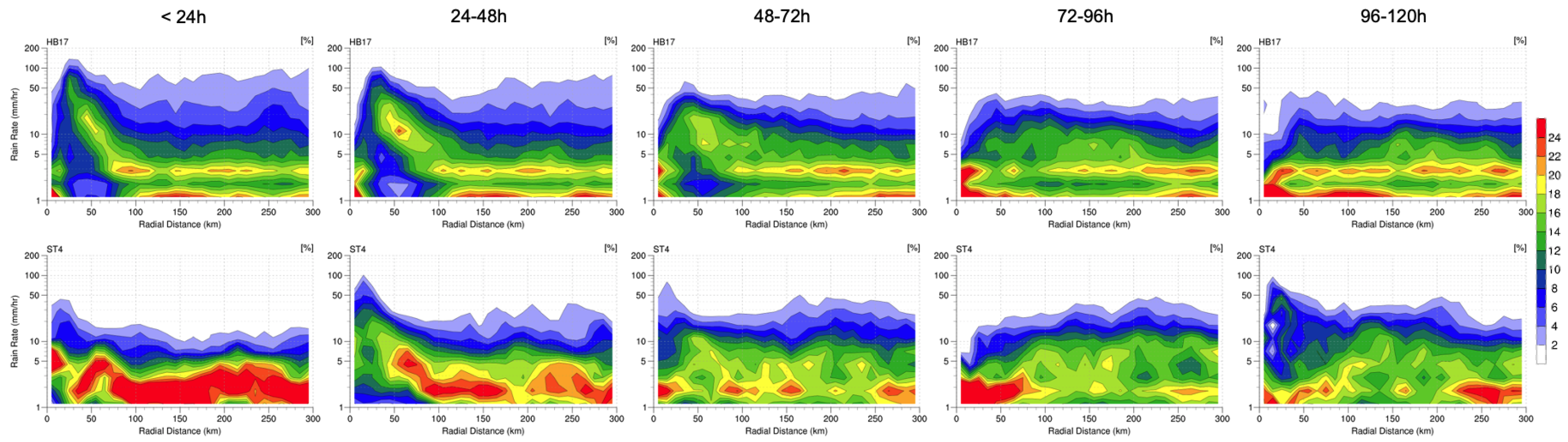
The PDF, the CDF, and the CFRD take the entire forecast cycles into account and provide overall performance on rain-rate frequency. In order to further examine the temporal changes of rain-rate distributions, we calculated the CFRD profiles averaged within 24-h intervals: the period of time within the first 24 h represents the rain-rate frequency prior to the landfall, the 24 to 48 h shows the status during the landfall, and the rain-rate changes during weakening and dissipating are shown in the 48 to 120 h CFRDs. In Figure 11, HB17 (the first row) predicted a realistic rain-rate frequency from landfall to dissipation compared with the Stage IV results (the second row). Shown in the first column of Figure 11, HB17 may have overestimated the heavy rain rate at the core before landfall, but Stage IV might not be accurate over the ocean. Therefore, the overestimation of heavy rain-rate frequency in the core of HB17’s overall CFRD (Figure 10) might be partially contributed by this uncertainty of observations. Despite an underprediction of high rainfall totals in HB17 forecasts (Section 3.1), the rain rate frequencies were remarkably predicted in terms of radial distributions and temporal changes.

3.3. Precipitation Probabilities

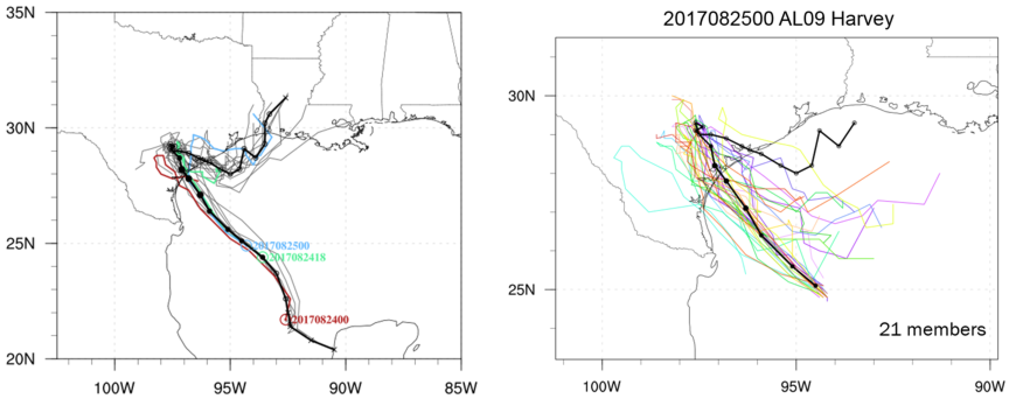
In order to minimize the uncertainty of deterministic forecasting, this study also evaluates an experiment of probabilistic precipitation forecasting using an HWRF ensemble model. This model generated 21 ensemble members (Figure 2 right panel), and most of the members show that Hurricane Harvey curved back to the Gulf of Mexico after making landfall. However, only a few members predicted the storm track moving towards Louisiana through the Gulf of Mexico. 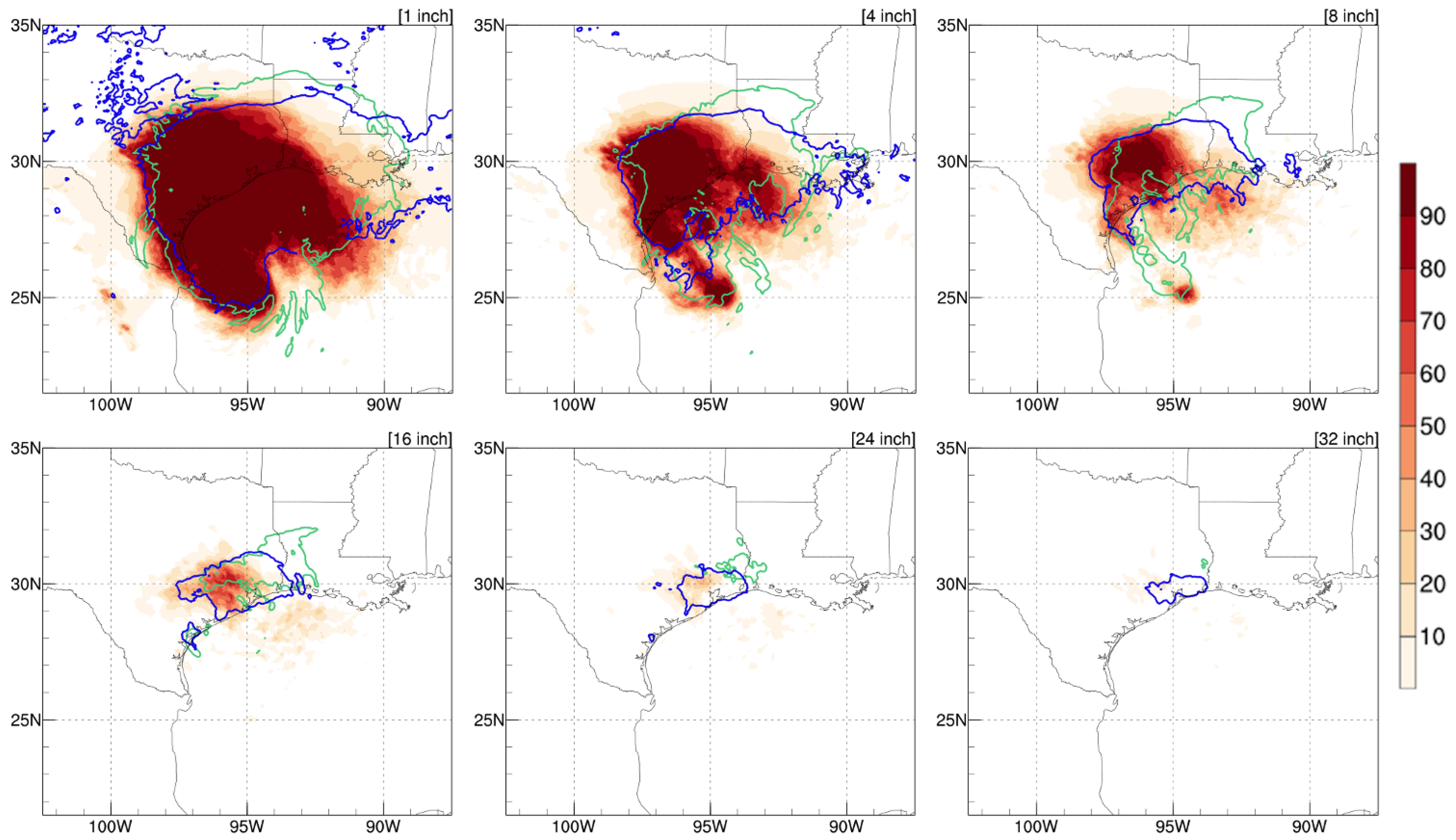Figure 12 shows the probabilistic precipitation forecasts of 1, 4, 8, 16, 24, and 32 inches compared to Stage IV (blue contours) and HB17 (green contours) at 0000 UTC 25 August. In general, H17E produced reasonable rainfall patterns and predicted realistic rainfall locations. The top 3 panels show 1-, 4-, and 8-inch accumulated rainfall probability. The predictions were mostly contained within Stage IV observations, except the rainfall in Louisiana and southern Mississippi was not successfully captured by the majority of ensemble members. HB17 shows accumulated rainfall is above 8 inches along the track in the Gulf of Mexico, but H17E predicts that the accumulated rainfall in this region is most likely in between 4 inches and 8 inches. The 16-inch accumulated rainfall panel indicates a similar result: even though most of the high possibility region is contained within the observation contours but the predicted region is not sufficient. Unlike the result of the deterministic run where the 16-inch prediction overextended to Louisiana, the probabilistic run only presents the rainfall over Houston and misses the area east of Houston. Moreover, in the 24-inch and 32-inch probabilistic panels, few members indicate that the location of these amounts of rainfall occurs around Houston. H17E matches Stage IV better than HB17, which predicted a peak rainfall closer to Louisiana. However, too few of the members show this extreme rainfall amount as the ensemble members unsuccessfully predicted Harvey’s intensity. The storm intensity was underestimated, which could contribute to the probability of extreme rainfall. This experiment shows that probabilistic rainfall prediction of areas exceeding certain thresholds considering several track possibilities can deliver more realistic extreme rainfall locations than HB17. However, in our case, H17E did not provide the correct rainfall amounts exceeding certain thresholds and missed the lighter rain totals over eastern Texas.

4. Discussion

This study demonstrated the performance and utility of the HWRF precipitation forecasts for Hurricane Harvey (2017) using a deterministic version (HB17) and a probabilistic version (H17E). These versions were compared with robust baselines (Stage IV, IMERG, and R-CLIPER) to show that HWRF is capable of producing realistic rainfall totals and improving the prediction of heavy rainfall locations. Overall, the HWRF precipitation forecasts for Harvey were encouraging. Details of the findings are discussed below:

4.1. Deterministic Hwrf Rainfall Prediction

Deterministic rainfall forecasts are useful because the models that make them can be configured at convective-scale resolutions to better simulate processes important for precipitation. HB17 produced realistic forecasts of rainfall patterns and rain rate distributions over land associated with Hurricane Harvey, including an intense and stationary outer rainband near Houston that had precipitation totals in excess of 32 inches over the forecast period. Although this rainband location was not perfectly predicted, this case study supports the utility of HWRF precipitation forecasts even in difficult scenarios, such as the landfall and subsequent stall of Harvey in southeastern Texas. Further investigation revealed a realistic radial distribution of rain rates and rain flux in Harvey, especially at larger radii where the intense rainband was located. Further modification of the HWRF physics may further improve precipitation forecasts. For example, the convection parameterization in HB17 may have contributed to a frequency of extreme rain rates that was higher than expected. It is recommended that HWRF be considered as QPF guidance for landfalling TCs.

4.2. Probabilistic Hwrf Rainfall Prediction

An advantage of probabilistic rainfall forecasting is that it comprehensively considers several possible atmospheric conditions to account for uncertainty and limited predictability in NWP models. H17E predicted the extreme rainfall location more reliably than HB17. However, the ensemble missed the rainfall in Louisiana, and the heavy rainfall probability was potentially low due to the weaker ensemble intensity forecasts. For practically interpolating the probabilistic outputs, the uncertainty between members should be taken into account. Extreme rainfall should be emphasized even when only a handful of members show the tendency. Also, utilizing an ensemble model with a higher number of members could possibly help to further improve estimates of uncertainty in extreme amounts, but relies on increased computational resources. Regardless, H17E has already shown the potential benefits of the HWRF probabilistic prediction for identifying extreme rainfall locations.

4.3. R-Cliper Rainfall Prediction

Due to the simplicity of the R-CLIPER model, the rainfall pattern was not well presented for Hurricane Harvey. R-CLIPER predicted that rainfall accumulated only along the track while Hurricane Harvey had a strong outer rainband. It is worthy to note that the computational cost of R-CLIPER is very small and this model was originally developed to serve as a climatological baseline for dynamic model rainfall evaluation. The TRMM mode of R-CLIPER rainfall is simply based on a storm intensity, and this method is highly efficient. However, the strongest rainfall does not necessarily happen within eyewall where the strongest wind is. Moreover, shear and topography effects are important elements for rainfall evaluation [3,12]. Hence, R-CLIPER can be further upgraded to increase its predictability within affordable computational cost. For example, an ensemble version of R-CLIPER or PHRaM can be developed to take different possibilities of extreme rainfall patterns into account.

4.4. The Limitations of Observational Data

Our study validated model performance against the observational data, which we assumed are the ground truth for rainfall amounts. However, there are limitations of data collections, which might increase the uncertainty of a model’s performance evaluation. In other words, Stage IV is a combination of rain gauge and radar datasets. Rain gauges might not be fully functional during severe weather events, and they only can collect data on land at certain locations. Like gauges, radar sensors only cover a certain range and have limited data over the ocean. Thus, even though Stage IV has a better resolution compared to other datasets, Stage IV is limited to in-land rainfall evaluation. To overcome this limitation, we also examined model performance against IMERG satellite data, which provides rainfall observations over the ocean. However, the drawback of this data is that its resolution is lower than Stage IV.

5. Conclusions

Overall, this case study of Hurricane Harvey shows that HWRF is capable of producing realistic precipitation, including patterns, totals, and rain rate distributions. In particular, the deterministic HWRF model can capture heavy precipitation in outer rainbands successfully. Moreover, probabilistic forecasts can potentially enhance the prediction skill of extreme rainfall locations. In general, low track errors are an ingredient for good QPF forecasts. However, QPF performance also relies on varied atmospheric conditions other than rainfall parameterization [20]. To further improve the HWRF QPF, more examination of the convection, microphysics, and rainfall-relative parameterizations are required. Meanwhile, probabilistic rainfall forecasts from the ensemble model may be an alternative way to further improve QPF by considering multiple atmospheric scenarios. HWRF may be leveraged as a real-time rainfall forecasting tool to provide useful guidance for disaster management. It is important to note that this study only discussed one TC, and this evaluation procedure can be extended to multiple cases to increase the confidence of these HWRF QPF results. Furthermore, the procedure is applicable for any NWP system, such as the NOAA next generation models. As precipitation forecasts from hurricane models become more reliable, this manuscript can serve as a roadmap for how to improve QPF guidance in the future.

References

1. Rappaport, E.N. Fatalities in the United States from Atlantic Tropical Cyclones: New Data and Interpretation. Bull. Am. Meteorol. Soc. 2014, 95, 341–346. [Google Scholar] [CrossRef]
2. Lonfat, M.; Marks, F.D.; Chen, S.S. Precipitation Distribution in Tropical Cyclones Using the Tropical Rainfall Measuring Mission (TRMM) Microwave Imager: A Global Perspective. Mon. Weather Rev. 2004, 132, 1645–1660. [Google Scholar] [CrossRef]
3. Lonfat, M.; Rogers, R.; Marchok, T.; Marks, F.D. A Parametric Model for Predicting Hurricane Rainfall. Mon. Weather Rev. 2007, 135, 3086–3097. [Google Scholar] [CrossRef]
4. Marchok, T.; Rogers, R.; Tuleya, R. Validation Schemes for Tropical Cyclone Quantitative Precipitation Forecasts: Evaluation of Operational Models for U.S. Landfalling Cases. Weather Forecast. 2007, 22, 726–746. [Google Scholar] [CrossRef] [Green Version]
5. Simpson, R.H.; Saffir, H. The Hurricane Disaster—Potential Scale. Weatherwise 1974, 27, 169–186. [Google Scholar] [CrossRef]
6. Murphy, J.D. August–September 2017 Hurricane Harvey; Noaa Service Assessment; NOAA/NWS: Silver Spring, MD, USA, 2018. Available online: https://www.weather.gov/media/publications/assessments/harvey6-18.pdf (accessed on 15 April 2019).
7. Blake, E.S.; Zelinsky, D.A. Hurricane Harvey (AL092017); National Hurricane Center tropical cyclone report; National Hurricane Center: Miami, FL, USA, 2018; p. 77.
8. Zhang, W.; Villarini, G.; Vecchi, G.; Smith, J.A. Urbanization exacerbated the rainfall and flooding caused by hurricane Harvey in Houston. Nature 2018, 563, 384–388. [Google Scholar] [CrossRef] [PubMed]
9. van Oldenborgh, G.J.; van der Wiel, K.; Sebastian, A.; Singh, R.; Arrighi, J.; Otto, F.; Haustein, K.; Li, S.; Vecchi, G.; Cullen, H. Attribution of extreme rainfall from Hurricane Harvey, August 2017. Environ. Res. Lett. 2017, 12, 124009. [Google Scholar] [CrossRef]
10. Knutson, T.; Camargo, S.J.; Chan, J.C.L.; Emanuel, K.; Ho, C.H.; Kossin, J.; Mohapatra, M.; Satoh, M.; Sugi, M.; Walsh, K.; et al. Tropical Cyclones and Climate Change Assessment: Part I: Detection and Attribution. Bull. Am. Meteorol. Soc. 2019, 100, 1987–2007. [Google Scholar] [CrossRef] [Green Version]
11. Emanuel, K. Assessing the present and future probability of Hurricane Harvey’s rainfall. Proc. Natl. Acad. Sci. USA 2017, 114, 12681–12684. [Google Scholar] [CrossRef] [Green Version]
12. Rogers, R.; Marks, F.; Marchok, T. Tropical Cyclone Rainfall. In Encyclopedia of Hydrological Sciences; Chapter Part 3. Meteorology and Climatology; American Cancer Society: Atlanta, GA, USA, 2009; p. 24. [Google Scholar] [CrossRef]
13. Stanski, H.R.; Wilson, L.J.; Burrows, W.R. Survey of Common Verification Methods in Meteorology; Wmo/td no. 358; WMO: Geneva, Switzerland, 1989. [Google Scholar]
14. Schaefer, J.T. The Critical Success Index as an Indicator of Warning Skill. Weather Forecast. 1990, 5, 570–575. [Google Scholar] [CrossRef] [Green Version]
15. Olson, D.A.; Junker, N.W.; Korty, B. Evaluation of 33 Years of Quantitative Precipitation Forecasting at the NMC. Weather Forecast. 1995, 10, 498–511. [Google Scholar] [CrossRef] [Green Version]
16. Wilks, D.S. Statistical Methods in the Atmospheric Sciences; Academic Press: Cambridge, MA, USA, 1995; p. 467. [Google Scholar]
17. Jankov, I.; Gallus, W.A.; Segal, M.; Shaw, B.; Koch, S.E. The Impact of Different WRF Model Physical Parameterizations and Their Interactions on Warm Season MCS Rainfall. Weather Forecast. 2005, 20, 1048–1060. [Google Scholar] [CrossRef]
18. Aligo, E.A.; Gallus, W.A.; Segal, M. On the Impact of WRF Model Vertical Grid Resolution on Midwest Summer Rainfall Forecasts. Weather Forecast. 2009, 24, 575–594. [Google Scholar] [CrossRef] [Green Version]
19. Wang, C.C. On the Calculation and Correction of Equitable Threat Score for Model Quantitative Precipitation Forecasts for Small Verification Areas: The Example of Taiwan. Weather Forecast. 2014, 29, 788–798. [Google Scholar] [CrossRef]
20. Ebert, E.E.; Damrath, U.; Wergen, W.; Baldwin, M.E. The WGNE Assessment of Short-term Quantitative Precipitation Forecasts. Bull. Am. Meteorol. Soc. 2003, 84, 481–492. [Google Scholar] [CrossRef]
21. Tuleya, R.E.; DeMaria, M.; Kuligowski, R.J. Evaluation of GFDL and Simple Statistical Model Rainfall Forecasts for U.S. Landfalling Tropical Storms. Weather Forecast. 2007, 22, 56–70. [Google Scholar] [CrossRef]
22. Weisman, M.L.; Skamarock, W.C.; Klemp, J.B. The Resolution Dependence of Explicitly Modeled Convective Systems. Mon. Weather Rev. 1997, 125, 527–548. [Google Scholar] [CrossRef]
23. Roberts, N.M.; Lean, H.W. Scale-Selective Verification of Rainfall Accumulations from High-Resolution Forecasts of Convective Events. Mon. Weather Rev. 2008, 136, 78–97. [Google Scholar] [CrossRef]
24. Wu, D.; Peters-Lidard, C.; Tao, W.K.; Petersen, W. Evaluation of NU-WRF Rainfall Forecasts for IFloodS. J. Hydrometeorol. 2016, 17, 1317–1335. [Google Scholar] [CrossRef]
25. Peters-Lidard, C.D.; Kemp, E.M.; Matsui, T.; Santanello, J.A.; Kumar, S.V.; Jacob, J.P.; Clune, T.; Tao, W.K.; Chin, M.; Hou, A.; et al. Integrated modeling of aerosol, cloud, precipitation and land processes at satellite-resolved scales. Environ. Model. Softw. 2015, 67, 149–159. [Google Scholar] [CrossRef] [Green Version]
26. Gopalakrishnan, S.G.; Marks, F.; Zhang, X.; Bao, J.W.; Yeh, K.S.; Atlas, R. The Experimental HWRF System: A Study on the Influence of Horizontal Resolution on the Structure and Intensity Changes in Tropical Cyclones Using an Idealized Framework. Mon. Weather Rev. 2011, 139, 1762–1784. [Google Scholar] [CrossRef]
27. Gopalakrishnan, S.G.; Goldenberg, S.; Quirino, T.; Zhang, X.; Marks, F.; Yeh, K.S.; Atlas, R.; Tallapragada, V. Toward Improving High-Resolution Numerical Hurricane Forecasting: Influence of Model Horizontal Grid Resolution, Initialization, and Physics. Weather Forecast. 2012, 27, 647–666. [Google Scholar] [CrossRef]
28. Gopalakrishnan, S.G.; Marks, F.; Zhang, J.A.; Zhang, X.; Bao, J.W.; Tallapragada, V. A Study of the Impacts of Vertical Diffusion on the Structure and Intensity of the Tropical Cyclones Using the High-Resolution HWRF System. J. Atmos. Sci. 2013, 70, 524–541. [Google Scholar] [CrossRef]
29. Biswas, M.K.; Bernardet, L.; Abarca, S.; Ginis, I.; Grell, E.; Kalina, E.; Kwon, Y.; Liu, B.; Liu, Q.; Marchok, T.; et al. Hurricane Weather Research and Forecasting (HWRF) Model: 2017 Scientific Documentation. NCAR Techn. Note NCAR/TN-544+STR 2017. [Google Scholar] [CrossRef]
30. Gopalakrishnan, S.; Toepfer, F.; Forsythe-Newell, S.; Marks, M.D.F.; Rappaport, E.N.; Tallapragada, V.; Franklin, J.; Abarca, S.; Aksoy, A.; Alaka, G., Jr.; et al. 2017 HFIP R&D Activities Summary: Recent Results and Operational Implementation; Hfip Technical Report; NOAA: Silver Spring, MD, USA, 2018. Available online: http://www.hfip.org/documents/HFIP_AnnualReport_FY2017.pdf (accessed on 1 May 2020).
31. Tallapragada, V.; Kieu, C.; Trahan, S.; Zhang, Z.; Liu, Q.; Wang, W.; Tong, M.; Zhang, B.; Strahl, B. Forecasting Tropical Cyclones in the Western North Pacific Basin Using the NCEP Operational HWRF: Real-Time Implementation in 2012. Weather Forecast. 2015, 30, 1355–1373. [Google Scholar] [CrossRef]
32. Zhang, Z.; Tallapragada, V.; Kieu, C.; Trahan, S.; Wang, W. HWRF Based Ensemble Prediction System Using Perturbations from GEFS and Stochastic Convective Trigger Function. Trop. Cyclone Res. Rev. 2014, 3, 145–161. [Google Scholar] [CrossRef]
33. Zhang, Z. Introduction to the HWRF-Based Ensemble Prediction System. 2018 Hurricane WRF Tutorial; NCEP/NOAA/EMC. 2018, p. 31. Available online: https://dtcenter.org/HurrWRF/users/tutorial/2018_NCWCP_tutorial/lectures/21-HWRFtutJan2018_HWRFEnsemble_ZZhang.pdf (accessed on 1 March 2020).
34. Zhang, X.; Quirino, T.; Yeh, K.; Gopalakrishnan, S.; Marks, F.; Goldenberg, S.; Aberson, S. HWRFx: Improving Hurricane Forecasts with High-Resolution Modeling. Comput. Sci. Eng. 2011, 13, 13–21. [Google Scholar] [CrossRef]
35. Zhang, X.; Gopalakrishnan, S.G.; Trahan, S.; Quirino, T.S.; Liu, Q.; Zhang, Z.; Alaka, G.; Tallapragada, V. Representing Multiple Scales in the Hurricane Weather Research and Forecasting Modeling System: Design of Multiple Sets of Movable Multilevel Nesting and the Basin-Scale HWRF Forecast Application. Weather Forecast. 2016, 31, 2019–2034. [Google Scholar] [CrossRef]
36. Alaka, G.J.; Zhang, X.; Gopalakrishnan, S.G.; Goldenberg, S.B.; Marks, F.D. Performance of Basin-Scale HWRF Tropical Cyclone Track Forecasts. Weather Forecast. 2017, 32, 1253–1271. [Google Scholar] [CrossRef]
37. Lin, Y.; Mitchell, K.E. The NCEP Stage II/IV Hourly Precipitation Analyses: Development and Applications. In Proceedings of the Extended Abstracts, Nineteenth Conf. on Hydrology, American Meteorological Society, San Diego, CA, USA, 9–13 January 2005. [Google Scholar]
38. Fulton, R.A.; Breidenbach, J.P.; Seo, D.J.; Miller, D.A.; O’Bannon, T. The WSR-88D Rainfall Algorithm. Weather Forecast. 1998, 13, 377–395. [Google Scholar] [CrossRef]
39. Nelson, B.R.; Prat, O.P.; Seo, D.J.; Habib, E. Assessment and Implications of NCEP Stage IV Quantitative Precipitation Estimates for Product Intercomparisons. Weather Forecast. 2016, 31, 371–394. [Google Scholar] [CrossRef]
40. Huffman, G.J.; Bolvin, D.T.; Braithwaite, D.; Hsu, K.; Joyce, R.; Kidd, C.; Nelkin, E.J.; Sorooshian, S.; Tan, J.; Xie, P. NASA Global Precipitation Measurement (GPM) Integrated Multi-satellitE Retrievals for GPM (IMERG). Algorithm Theoretical Basis Document (atbd), NASA; 2017. Available online: https://pmm.nasa.gov/sites/default/files/document_files/IMERG_ATBD_V5.1.pdf (accessed on 15 April 2019).
41. Cui, W.; Dong, X.; Xi, B.; Feng, Z.; Fan, J. Can the GPM IMERG Final Product Accurately Represent MCSs’ Precipitation Characteristics over the Central and Eastern United States? J. Hydrometeorol. 2020, 21, 39–57. [Google Scholar] [CrossRef]
42. Maranan, M.; Fink, A.H.; Knippertz, P.; Amekudzi, L.K.; Atiah, W.A.; Stengel, M. A Process-Based Validation of GPM IMERG and Its Sources Using a Mesoscale Rain Gauge Network in the West African Forest Zone. J. Hydrometeorol. 2020, 21, 729–749. [Google Scholar] [CrossRef]
43. Marks, F.; Kappler, G.; DeMaria, M. Development of a Tropical Cyclone Rainfall Climatology and Persistence (R-CLIPER) Model. In Proceedings of the 25th Conference on Hurricanes and Tropical Meteorology, San Diego, CA, USA, 29 April–3 May 2002; p. 7D.2. Available online: https://ams.confex.com/ams/pdfpapers/35695.pdf (accessed on 15 June 2019).
Figure 1. Track performance for Hurricane Harvey. HB17 is shown in red lines with triangle markers, H217 is purple with diamond markers, and GFS is blue with square markers. The left panel shows the absolute track errors and the right panel shows the track skill using H217 as a baseline.
Atmosphere 11 00666 g001
Figure 2. Left panel: HB17 deterministic track forecasts for Hurricane Harvey in the Gulf of Mexico: 0000 UTC 24 August 2017 (red line), 1800 UTC 24 August 2017 (green), and 0000 UTC 25 August 2017 (blue). Gray lines represent the track forecasts from unselected cycles. Right panel: H17E ensemble track forecasts for Hurricane Harvey on 0000 UTC 25 August 2017 are shown in colored lines. The black line is the Best Track.
Atmosphere 11 00666 g002
Figure 3. Rain swaths for HB17 (1st column), Stage IV (2nd column), IMERG (3rd column), and R-CLIPER (4th column). The first row represents the model forecast start time at 0000 UTC 24 August 2017, the second row is at 1800 UTC 24 August 2017, and the third row is at 0000 UTC 25 August 2017. Black lines are the forecast/best tracks of models/observations. The markers are 6 hourly storm locations. The maximum values of accumulated rainfall are shown in the top-right corner of each panel.
Atmosphere 11 00666 g003
Figure 4. Rain swath difference between HB17 and observational datasets. The difference between HB17 and Stage IV data are shown in the left panels. The right panels show the different plots of HB17 and IMERG. Red indicates overestimation from the HB17 model and blue is underestimation.
Atmosphere 11 00666 g004
Figure 5. Colored lines are the critical success index (CSI) corresponding to three selected cycles: blue is 0000 UTC 24 August 2017, red is 1800 UTC 24 August 2017, and yellow is 0000 UTC 25 August 2017. The black line is the averaged CSI. The x-axis shows the accumulated rainfall thresholds.
Atmosphere 11 00666 g005
Figure 6. Similar to Figure 5 but for bias scores.
Atmosphere 11 00666 g006
Figure 7. Radial distribution of average rain rate of Hurricane Harvey. HB17’s distribution is the red line, R-CLIPER is green, and Stage IV is blue.
Atmosphere 11 00666 g007
Figure 8. Radial distribution of rain flux of Hurricane Harvey. Similar to Figure 7.
Atmosphere 11 00666 g008
Figure 9. Probability distribution functions (PDF) and CDF of decibel rain rates (dBR). The blue line is PDF and the dashed red line is CDF. The 50th percentile of CDF is indicated via yellow points and the 75th percentile via green points. From the left to the right panel, the results are from HB17, Stage IV, and R-CLIPER sequentially.
Atmosphere 11 00666 g009
Figure 10. Contoured frequency by radial distance (CFRD). The distance interval is 10 km starting from 0 to 300 km, and the rain rate interval is 2 dBR. From the left to the right panel, the results are from HB17, Stage IV, and R-CLIPER sequentially.
Atmosphere 11 00666 g010
Figure 11. Similar to Figure 10 but for a 24-h interval. The top row is HB17’s CFRD and the bottom row is Stage IV. The first column is calculated from the first 24 h, the second is between 24 to 48 h, the third is 48 to 72 h, the fourth is 72 to 96 h, and the last is 96 to 120 h.
Atmosphere 11 00666 g011
Figure 12. 126-h probabilistic rainfall for Harvey cycle 0000 UTC 25 August. Thresholds are 1, 4, 8, 16, 24, and 32 inches for panels from left to right and top to bottom. The blue lines are contours of thresholds from Stage IV, and the green lines are from HB17. The shaded contours are from H17E. The corresponding H17E, HB17, and Best Track positions are shown in Figure 2.
Atmosphere 11 00666 g012