Article

Statistical Learning of the Worst Regional Smog Extremes with Dynamic Conditional Modeling

1
School of Statistics and Mathematics, Central University of Finance and Economics, Beijing 100081, China
2
Department of Operations Research and Financial Engineering, Princeton University, Princeton, NJ 08540, USA
3
Department of Statistics, University of Wisconsin, Madison, WI 53706, USA
*
Author to whom correspondence should be addressed.
These authors contributed equally to this work.
Atmosphere 2020, 11(6), 665; https://doi.org/10.3390/atmos11060665
Submission received: 19 May 2020 / Revised: 11 June 2020 / Accepted: 19 June 2020 / Published: 22 June 2020
(This article belongs to the Special Issue Statistical Approaches to Investigate Air Quality)

Abstract

:
This paper is concerned with the statistical learning of the extreme smog (PM 2.5 ) dynamics of a vast region in China. Differently from classical extreme value modeling approaches, this paper develops a dynamic model of conditional, exponentiated Weibull distribution modeling and analysis of regional smog extremes, particularly for the worst scenarios observed in each day. To gain higher modeling efficiency, weather factors will be introduced in an enhanced model. The proposed model and the enhanced model are illustrated with temporal/spatial maxima of hourly PM 2.5 observations each day from smog monitoring stations located in the Beijing–Tianjin–Hebei geographical region between 2014 and 2019. The proposed model performs more precisely on fittings compared with other previous models dealing with maxima with autoregressive parameter dynamics, and provides relatively accurate prediction as well. The findings enhance the understanding of how severe extreme smog scenarios can be and provide useful information for the central/local government to conduct coordinated PM 2.5 control and treatment. For completeness, probabilistic properties of the proposed model were investigated. Statistical estimation based on the conditional maximum likelihood principle is established. To demonstrate the estimation and inference efficiency of studies, extensive simulations were also implemented.

1. Introduction

Modeling extreme climatic conditions [1,2], extreme weather [3,4,5,6,7,8], and rather harmful air pollutants, together with their social, economic, political, and human impacts, is a contemporary research topic. It was concluded by [9] that extreme weather is the new normal. References [10,11] studied the air quality in the USA, and air pollution and health effects in a pyramid figure of effects. Smog as a more serious type of harmful air pollutant has been drawing more and more attention recently. Studies on the masses and chemical compositions, as well as the concentrations, formation, and source of smog have been done [12,13,14,15,16,17,18,19]. Considering the significant impact that some meteorological conditions may have on the PM 2.5 concentrations [20,21,22], statistical approaches, as well as physical and chemical ones, were also conducted [23,24,25]. Except for the studies based on annual averaged PM 2.5 data [26,27,28], the cases when extreme smog happens are especially concerned [29,30,31,32,33]. For example, public attitudes and responses to the first two red warnings for air pollution in Beijing in 2015 were examined [34].
China’s smog problem stands out in its extremely high frequency, long duration, and high concentration. There are eleven long-lasting rounds of severe smog in 2015, which occurred mainly during the last two months of that year. On 30th November 2015, the PM 2.5 concentration in Beijing and the south of Hebei exceeded 900 μ g/m 3 and even reached 976 μ g/m 3 at Liuli River station, Beijing. The worst smog in 2016 started from 16th December and ended on 21st, covering 17 provinces; i.e., over one seventh of the national territory area. Three fourths of the cities are located in the Beijing–Tianjin–Hebei region and its surrounding regions. The PM 2.5 concentration in the downtown of Shijiazhuang city even broke 1000 μ g/m 3 . These observations clearly direct us to be more concerned with the statistical learning of extreme smog (PM 2.5 ) dynamics of a vast region in China. For example, classical extreme value analysis to hourly PM 2.5 data from 2014 to 2016 in China have been obtained [35]. It is also worth noting that the smog problem is not a unique phenomenon in China. It occurs elsewhere in the world, especially in developing countries; e.g., Dehli, India [36].
Understanding the extreme features of smog problems in China is very important since severe smog levels are more dangerous than ordinary levels and will do greater harm to China’s public health [37,38,39,40,41,42]. For example, in 2013, 83 % of the whole population in China was exposed to the air pollution with PM 2.5 level exceeding 35 μ g/m 3 , which might cause 1.3 million premature mortalities [43]. The smog also causes a significant economic loss for China [44,45] and even for the whole world [46,47].
Using classical extreme value theory, one could fit the generalized extreme value distribution to extreme observations recorded from each of those hundreds of smog monitoring stations. Recently, Dombry [48] studied properties of the maximum likelihood estimators for the extreme value index within the block maxima framework. Studies [49,50] are the most recent ones dealing with spatial extremes and processes. Study [51] proposed a dynamic modeling approach, the autoregressive conditional Fréchet (AcF) model, for maxima of daily negative log returns of 100 stocks in S&P100. These new models and modeling approaches can certainly be applied to the extreme observations in smog extremes in this study. However, static extreme value models do not offer a dynamic view and may be of less interest to administrators; in addition, the AcF model does not have good performance in climate extremes either. Different from published work in the literature, a new study approach is applied to smog extremes in our work, which intends to integrate a new type of extreme value modeling and dynamic modeling into a dynamic conditional distribution modeling and analysis of regional smog extremes, particularly the worst scenarios observed in each day. The results show a significant improvement compared with using existing extreme value modeling approaches. In addition, weather factors will be introduced in the model to gain higher modeling efficiency. The proposed model and the enhanced model are illustrated with real data of hourly PM 2.5 observations during 2014–2019 from smog monitoring stations located in the Beijing–Tianjin–Hebei geographical region. In particular, we studied the worst smog dynamic scenarios in the vast region of Beijing–Tianjin–Hebei in China. For joint regional extreme event monitoring and control, knowing first what can be the worst scenario in a day clearly will be very useful for administrators to decide whether or not to make warnings and some necessary control treatments. This paper enhances the understanding of how severe extreme smog scenarios can be and provide useful information for the central/local government to conduct coordinated PM 2.5 control and treatment. In the literature, researchers have paid much attention to extreme values in environmental studies; e.g., extreme temperature [2], precipitation [2,4,5,6], snowfall [52], and biomedical physics in brain image analysis [53], among many others. Our new model can certainly find applications in these areas. On the other hand, our model can also be applicable to studying systematic risk in financial systems [54], which is a contemporary research topic. Moreover, in terms of systematic risk study in air-quality control and treatment in regional risk and hazard management, our model can be very useful.

Roadmap

The rest of the paper is organized as follows. Section 2 conducts a preliminary analysis of smog in a vast region of Beijing–Tianjin–Hebei. In Section 3, we introduce our dynamic model by specifying a latent independent standard random process of standard Weibull random variables. Probabilistic properties of stationarity and ergodicity of the proposed model are investigated. Statistical estimation based on the conditional maximum likelihood principle is established. To demonstrate the estimation and inference efficiency of studies, extensive simulations are implemented in Section 4. Section 5 contains advanced modeling of smog extremes together with weather data. Section 6 offers conclusions of the paper regarding our applied study of smog extremes. Technical arguments are deferred to Appendix A.

2. Preliminary Analysis of Smog in the Vast Region of Beijing–Tianjin–Hebei
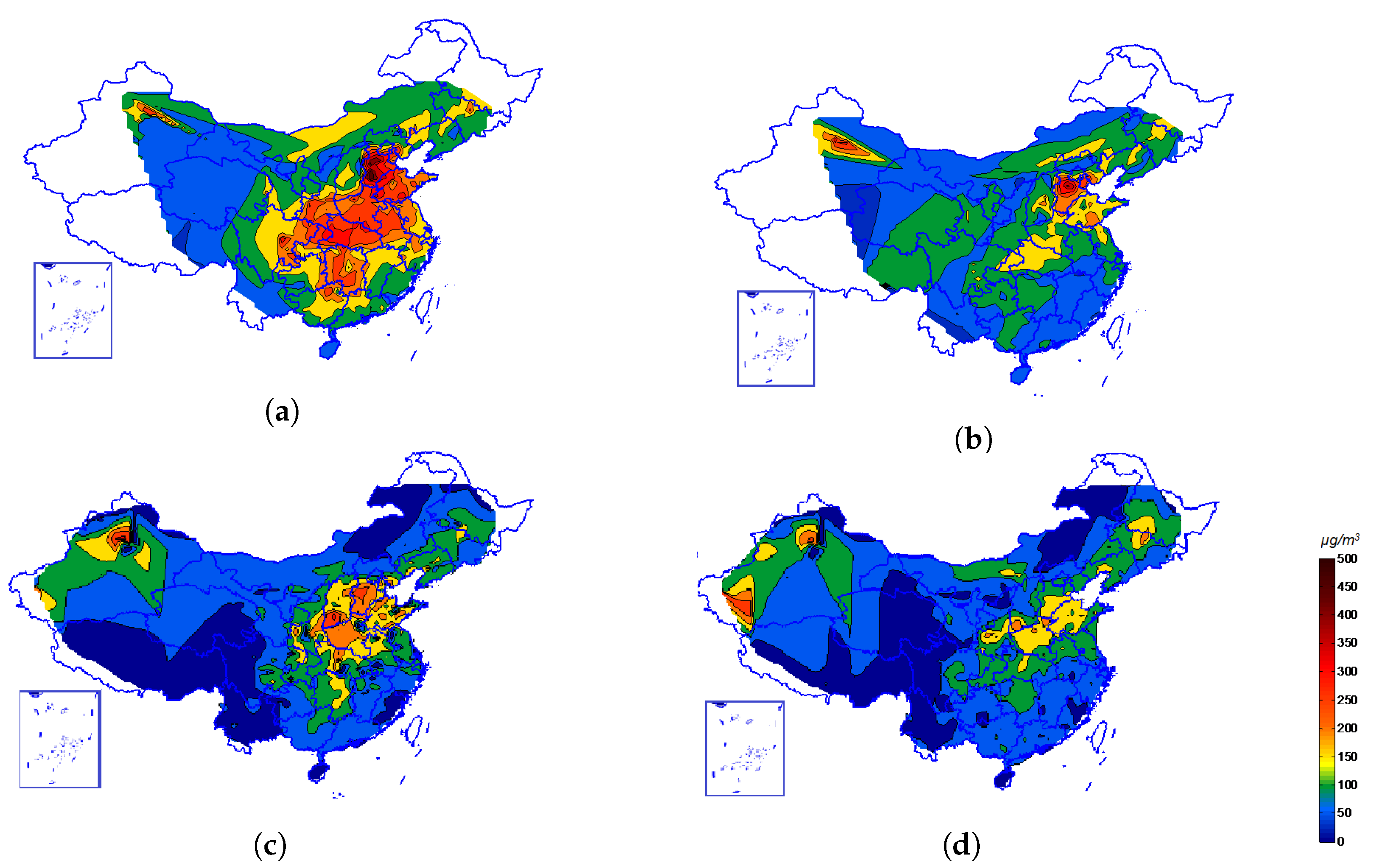
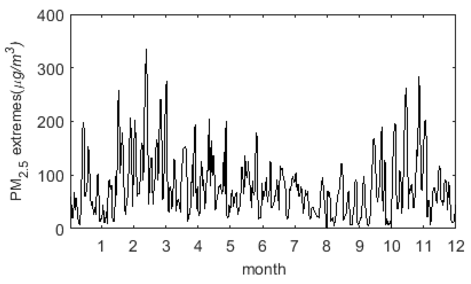
2.1. Which Time Scale of PM 2.5 Data Is to Be Analyzed?

When considering extreme smog as an extremely harmful air pollutant which may last a few hours in a day or last a couple of days, it becomes rather meaningful to study the hourly characteristics of radical smog movements, instead of daily traits. One can consider an analysis of daily data as well. We will not consider this time scale in this applied project.
To adequately demonstrate the variation of smog in different years, data from 2014 to 2019 are used to fit our proposed model. The first three months’ data of 2020 are used to check the predictability of our model. All the data are from the China National Environmental Monitoring Center. Due to technological testing, transition problems, hardware failure, possible delayed updates, etc., some of the data are missing and taken as non-observable smaller values to the observed daily maxima in this study.

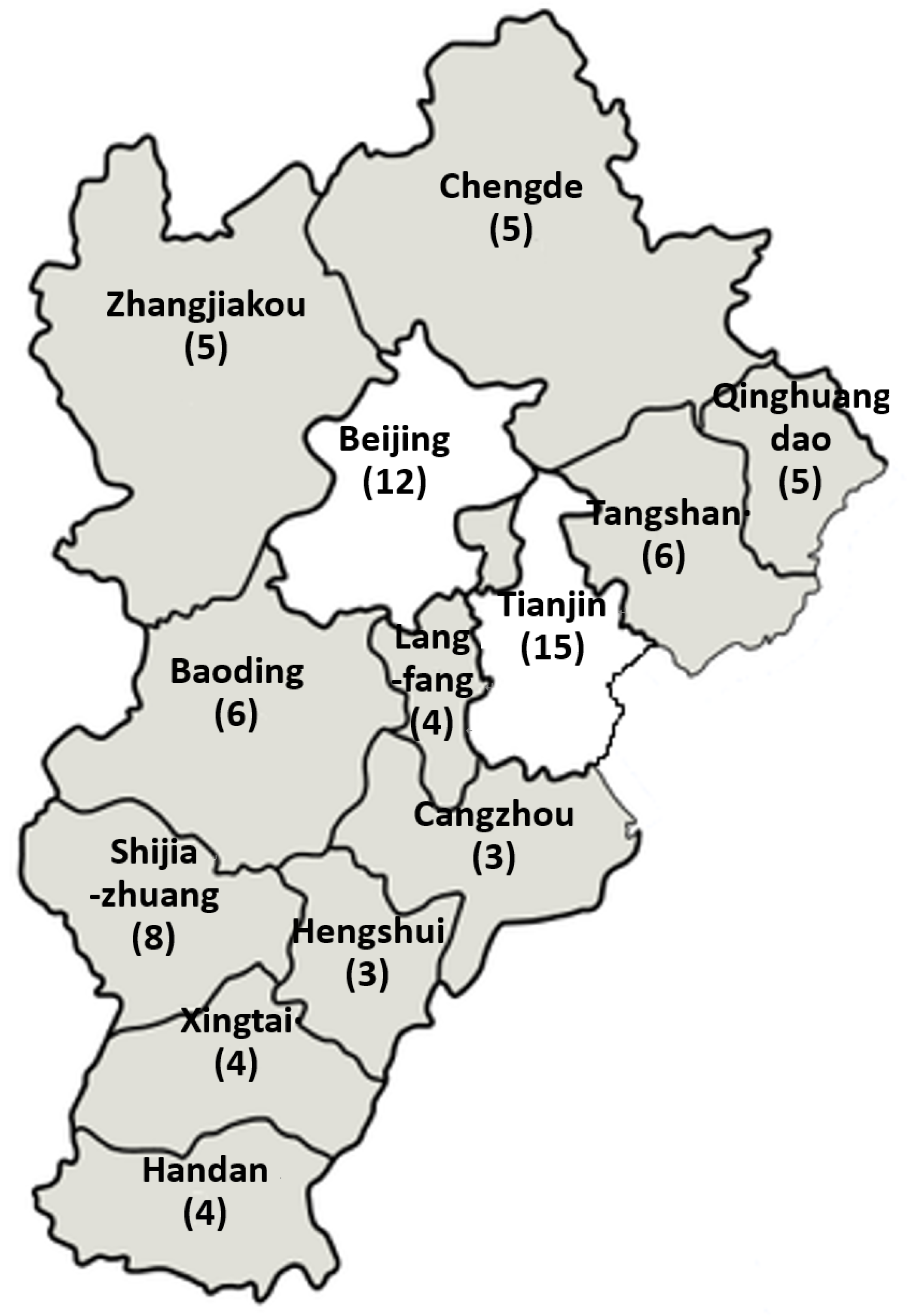
2.2. The Geographical Region to Be Focused on

Figure 1 demonstrates 90% quantile maps for January and December of 2014 and 2019 among the monitoring stations in mainland China.
As shown in Figure 1a, in January 2014, most of the monitored areas spanning the north, east, and middle of China (especially those red areas) had quantiles exceeding 150.4 μ g/m 3 , which is the starting point of the very unhealthy level of air quality according to the US standard [55]. There are five intervals of PM 2.5 levels according to the US (EPA) standard: (1) 35 μ g/m 3 is the highest PM 2.5 level for the good and moderate category; (2) the range from 35 to 55.4 μ g/m 3 is unhealthy for sensitive groups; (3) the range from 55.5 to 150.4 μ g/m 3 is unhealthy; (4) the range above 150.4 μ g/m 3 is widely viewed as very unhealthy; and (5) it is hazardous when the smog level is above 250.5 μ g/m 3 . We see then that south Hebei, Beijing, and Tianjin showed the highest smog levels with the 90% quantile values being close to an outstanding 500 μ g/m 3 , which is the maximum value given in the US standard. A similar conclusion can be drawn from Figure 1b is that in December 2014, south Hebei, Beijing, and Tianjin were still the worst air quality areas, although the quantiles of the smog values in most areas of China were much lower than their counterpart values in January. In January and December 2019 (as shown in Figure 1c,d respectively), the thresholds among all of China decreased significantly; that shows great improvement in extreme smog problems; south Hebei, Beijing, and Tianjin are still some of the key regions with the severest smog conditions (relatively higher threshold). Monthly 90% quantiles of 2015 and 2018 confirm this conclusion as well.
This study focuses on the smog problem in the Beijing–Tianjin–Hebei region; i.e., not all of mainland China, whose smog issues may be too diversified to draw consensus conclusions about. The importance of focusing the study on the smog problem in the Beijing–Tianjin–Hebei region is due to the fact that the areas are not only geographically connected but also economically significant in their immense contribution to China’s GDP (nearly 9% in 2019 with 8% of population). With the implementation of the collaborative development of the Beijing–Tianjin–Hebei region as a national strategy, the coordination among these three areas has been becoming more and more intimate. It has been taken as an indivisible whole, especially in the issues of smog prevention and control.
The smog problem in this region has been recognized on account of health concerns as early as in January 2013, when long-lasting severe smog prevailed and caused a significant increase in the number of patients with respiratory tract infections and allergic symptoms in hospitals and clinics in Beijing, Tianjin, and Shijiazhuang (the capital city of Hebei province). Research also indicated that bad air quality in northern China causes 5.5 years reductions of people’s life expectancy [56].
In the Beijing–Tianjin–Hebei region, besides two metropolitan cities, Beijing (the capital of China) and Tianjin (a major port city in northeastern China), there are 11 cities in Hebei province. Among these 11 cities, Zhangjiakou and Chengde are located in north Hebei; Qinghuangdao, Tangshan, and Cangzhou are in east Hebei; Baoding and Langfang are located in the middle of Hebei; Shijiazhuang, Hengshui, Xingtai, and Handan combine south Hebei. Their locations along with Beijing and Tianjin are shown in Figure 2. The number of smog monitoring stations in the region nearly remained the same during 2014–2019 (after deleting stations still under test, the numbers of valid stations are around 80 for all years). Worth noticing is that the station type is the key parameter to explain diurnal variability of atmospheric pollutants due to sources proximity. In this paper, however, since only the daily maxima of PM 2.5 across the whole region rather than a spatial model is considered, the station type and geographical information which describe the spatial relations are not used in the study.

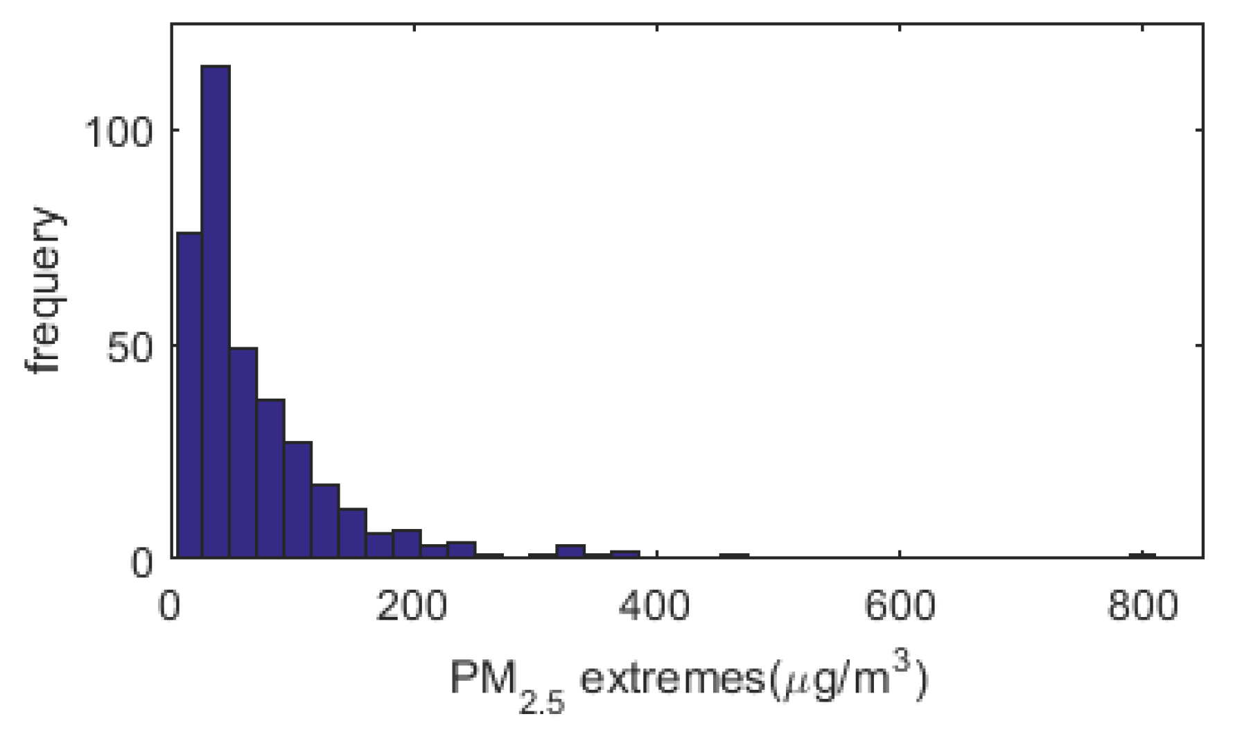
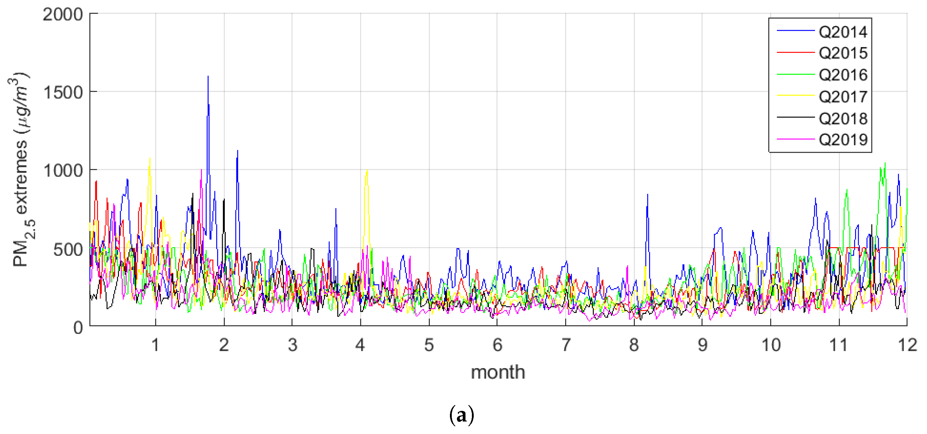
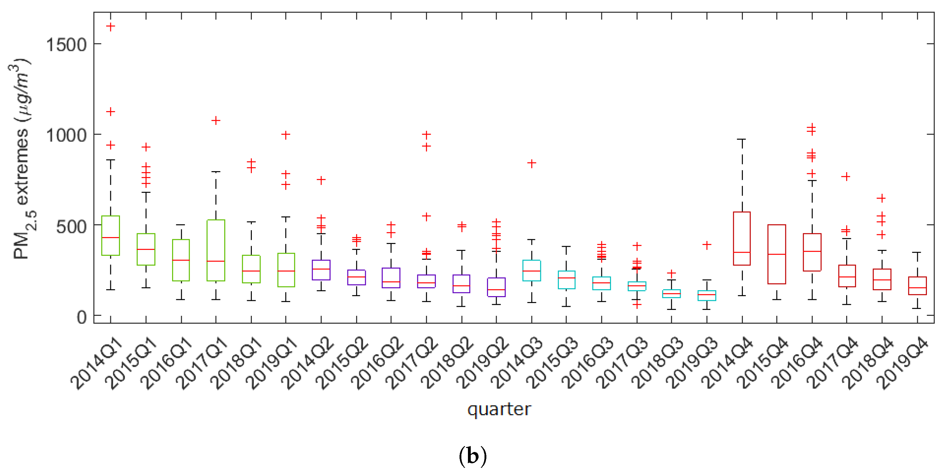
2.3. Why Model the Extremes Rather than the Average Levels?

This paper focuses on the extreme smog instead of average levels for two reasons. Firstly, the extreme smog rather than the ordinary smog affects the public health and causes more loss to the welfare of the whole society [36,38,41]. Secondly, when investigating the severity of smog, the results can be very different from the use of the annual averages or the extreme values of PM 2.5 data. Taking stations of Zhangjiakou and Chengde during 2014–2016 as an example, their annual average PM 2.5 levels rank as the best 30% among the whole country, showing relatively good air quality on average. However, as far as the means of extreme values (here extreme values refers to those PM 2.5 levels above the annual 90% quantile) are concerned, those stations belong to the worst third of the whole country. This difference in ranks gives two implications. On the one hand, the poorer grades using more extreme values than those using the annual averages show that the air quality of Zhangjiakou and Chengde may not be as good as one has thought; i.e., a city that performs well on average does not guarantee an absence of extreme smog. On the other hand, for Zhangjiakou and Chengde, while their extreme PM 2.5 levels were relatively lower most of the time, there were still a few occurrences of very high PM 2.5 levels to which considerable attention should be paid. The histograms of hourly PM 2.5 extreme values for those stations also confirm such arguments. One of those histograms at one representative station in Zhangjiakou in 2014 is given in Figure 3 as example.
For studies on the average PM 2.5 level rather than the extreme PM 2.5 value, we refer readers to [26,27,28].

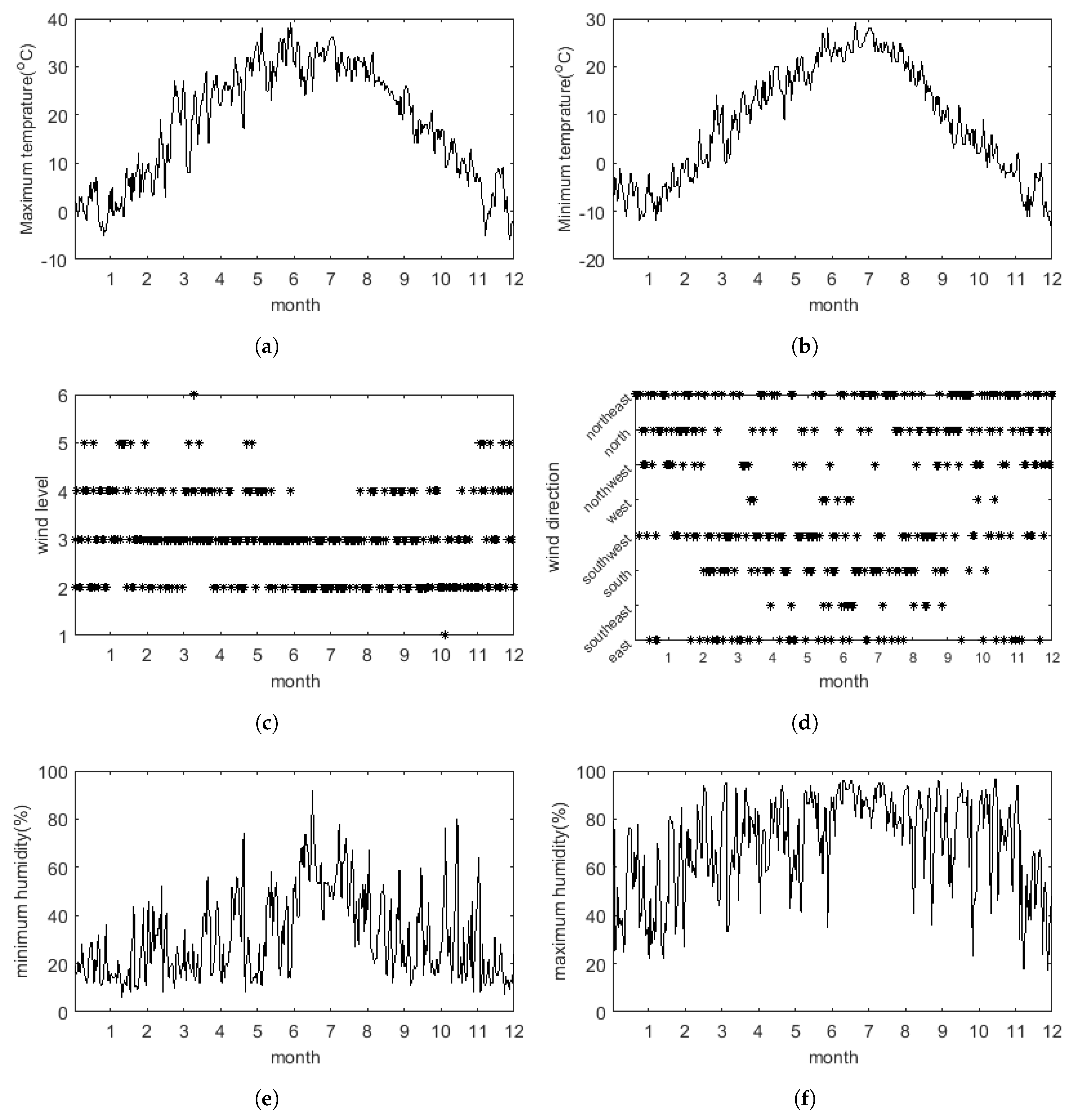
2.4. The Study Approach and the Inclusion of Meteorological Variables

With the established arguments in the prior section, this applied study focuses on the extreme values rather than the average values of PM 2.5 data. Ideally, one should build a model to describe extreme smog level dependencies among monitoring stations in the region. Then, all analyses and inferences, even policy recommendations, are to be based on the constructed model. To achieve this goal, a model builder has to consider many location/spatial parameters and extreme spatial dependencies, which can be very complicated and hardly implementable in a multivariate/spatial extreme value and time series context. We note that in the literature, workable and meaningful air quality models, including a comprehensive air quality model with extensions (CAMx), the community multiscale air quality modeling system (CMAQ), etc., have been developed for various applications and for developing public policies. In this study, we adopt an alternative approach in modeling regional extremes in a time series modeling framework. This paper tries to model the maximum PM 2.5 values of 24 h a day among all stations in the Beijing–Tianjin–Hebei region. Here, the extreme value represents the highest daily PM 2.5 concentration of the area as a whole. It is particularly useful when planning smog prevention and control measurements, since such measurements as well as the smog pre-warning systems are integrated and unified in the Beijing–Tianjin–Hebei region. The pre-warnings should be activated and corresponding measurements should also be taken so long as the predicted PM 2.5 level at one single station inside the region exceeds a specific breakpoint wherever the station is. In this circumstance, only the maximum value of the whole part rather than the particular concentrations of all individual stations is concerned.
The line graphs of the regional daily maximum (based on hourly observations) PM 2.5 levels from 2014 to 2019 are plotted in Figure 4a. It can be seen that extreme smog levels were much worse in 2014 since its extreme values were mostly much higher compared to the same period of the following five years. It is further demonstrated in Table 1 that the extreme values in 2014 have a much higher sample mean, median, maximum and standard deviation; they improved significantly in recent years with these statistics decreasing in general. More importantly, the maximum PM 2.5 levels over the years are persistent with an exceptional high value in 2014. Meanwhile, the skewness and kurtosis are persistently larger than those from a Gaussian distribution. The extreme values also show significant seasonality for all six years in that their sample means and standard deviations are much higher in the first and fourth seasons than the other two seasons, as shown in Figure 4b. We shall consider these dynamic characteristics in our model building.
In the literature, extensive research shows that climate factors may cause a significant impact on the PM 2.5 levels [20,21] at one location. These meteorological conditions include temperature, humidity (the humidity mentioned in this paper is relative humidity (%)), wind speed, wind direction, etc.; see [23,24]. Taking Beijing as an example, Figure 5 is the daily maximum PM 2.5 level of Beijing in 2018 that is computed using the hourly PM 2.5 levels among all monitoring stations in Beijing. The selected meteorological conditions are Beijing’s daily maximum and minimum temperature, daily maximum and minimum humidity, daily maximum wind levels, and its related wind direction in 2018, as shown in Figure 6. All the data are from the National Meteorological Information Center.
The annual maximum PM 2.5 level in Beijing is around 350 μ g/m 3 in 2018, which is much higher than the hazardous breakpoints (250 μ g/m 3 ) according to the US standard. Although the annual maximum of the PM 2.5 values in Beijing is lower than that of the regional extremes given in Table 1 (850 μ g/m 3 ), around one tenth of the daily regional extremes are observed from stations in Beijing. Actually, the locations of the highest daily regional extremes are well spread among cities in the Beijing–Tianjin–Hebei region, which exactly demonstrates that modeling the regional extremes instead of local PM 2.5 dynamics is very important. Besides, the smog in the first and last seasons is much more sever than that in the other two seasons; meanwhile, the daily minimum and maximum temperatures in the first and last seasons are much lower, showing potential negative correlations between the PM 2.5 level and temperature. As for wind and humidity, they affect the concentration of smog in different ways: it is known that humidity affects the atmospheric chemistry and the formation of secondary pollutants such as particulate matter and ozone. However, wind influences the concentrations of the trace gases, which react at rates determined by their concentrations. The fourth level wind coming from the north or northeast most often occurs in the first season, which tends to decrease the PM 2.5 level. However, the smog is still severe when the wind becomes weak. In this season, the differences between the daily maximum and minimum humidity are relatively larger (mainly caused by the lower minimum humidity), which is an adverse diffusion condition for the smog [57]. In the second and third seasons, winds with the third level coming from the south and south-west dominate. In these two seasons, the smog problem is much less sever and both the maximum and minimum humidity are relatively high (resulting in lower humidity difference). In the last season, winds seem to be weaker with the second level coming from the northeast, and both the daily maximum and minimum humidity are barely low (with a relatively smaller minimum humidity), which could be reasons leading to the severe smog. Generally speaking, it is observed that the lower the wind level and the higher the humidity difference (or the lower the minimum humidity), the higher the daily PM 2.5 extremes. These observations coincide with the general results from other studies [57,58]. More details about the specification of covariates (climate factors) when modeling the regional daily maximum PM 2.5 levels will be addressed in Section 5.2. The data source is also the National Meteorological Information Center.

3. Model Specification

Suppose X t i j is the PM 2.5 level on day t at time i (hour) of the jth station in a group containing m stations. Define Q t as
Q t = max 1 i 24 , j = 1 , , m X t i j .
An illustration of daily regional smog extremes’ time series { Q t } is given in Figure 4.
In the extreme value theory, under suitable conditions ([59]), the normalized maximum of a sequence (a group, a block, or an array) of random variables is distributed as a generalized extreme value (GEV) distribution in its limit when the size of the sequence tends to infinity. In view of the definition in Q t , random variables X t i j ’s are potentially showing time dependence and spatial dependence, and the distributions can be different. As a result, Q t can be hardly distributed as a GEV random variable, and the dependence between Q t and Q t 1 cannot be modeled using the models (e.g., [51,60]) developed for GEV distributed random variables.

3.1. The Proposed General Model

Inspired by the AcF model (autoregressive conditional Fréchet model) proposed by [51], we propose the following model for smog extremes modeling:
Q t = μ t + σ t Y t 1 / α t ,
where μ t is the lowest level of PM 2.5 in the region on day t, σ t > 0 is the scale parameter, α t > 0 is the shape parameter, and { Y t } t 0 is a sequence of i.i.d. exponentiated Weibull (unit exponential) random variables.
One notices that the standardized Q t , ( Q t μ t ) / σ t follows an exponentiated Weibull distribution with the shape parameter α t . By introducing the additional parameter α t , the distributions of Q t possess great variability and flexibility. In the literature, the exponentiated Weibull distribution has been applied to model climate extremes; e.g., in flood modeling in ([61]). Unlike the AcF model, wherein unit Fréchet distributions are assumed to capture the heavy-tailedness of financial data, Weilbull-distributed { Y t } s are considered here to fit the characteristics of smog data which are not necessarily being heavy-tailed. It has been observed in [35] that the station-wise extremes in the Beijing–Tianjin–Hebei region belong to the maximum domain of attraction of Weibull type, which leads to a reasonable assumption of Y t being standard Weibull distributed. To be more rigorous, we also fit the AcF model in Section 5 for comparison.
The next stage is to build a time series model for the { Q t } series. Following the arguments above and those in [51], to reduce the model complexity, we treat μ t as constant μ and interpret μ as the lowest level of PM 2.5 fpr all the time across the Beijing–Tianjin–Hebei region, and treat σ t and α t as dynamic.
Noticing that the smog levels can be affected by the past smog levels and weather conditions, we assume the following dynamic equations for the time varying parameters:
log σ t = β 0 + β 1 log σ t 1 + η σ ( Q t 1 , T p t 1 , H u t 1 , W d s t 1 , W d d t 1 ) ,
log α t = γ 0 + γ 1 log α t 1 + η α ( Q t 1 , T p t 1 , H u t 1 , W d s t 1 , W d d t 1 ) ,
in which T p t , H u t , W d s t , and W d d t denote the maximum temperature, minimum humidity, mode of wind speed, and mode of wind direction respectively. These four weather condition variables have been commonly discussed in the smog study literature; e.g., [62,63], and the references therein. Other weather factors can also be considered. However, adding too many variables increases the model complexity and weakens the effects of important variables. For this reason, we only focus on the dynamics of variables given in (3) and (4). We call model (2)–(4) the dynamic conditional Weibull (DCW) model. In this paper, we consider functions η σ ( . ) and η α ( . ) defined in (3) and (4) as exponential functions which are widely adopted in the literature, e.g., [51], due to their flexibilities in functional properties of boundedness, differentiability, and monotonicity. It is worth noting that the functions of η σ ( . ) and η α ( . ) given in (3) and (4) can also take other forms, as long as they meet some conditions that guarantee the dynamic processes being stationary and ergodic. For clarity and simplicity in the proofs of stationarity and ergodicity, we first omit terms related to weather factors and express model (2)–(4) as:
log σ t = β 0 + β 1 log ( σ t 1 ) + β 2 exp ( β 3 Q t 1 ) ,
log α t = γ 0 + γ 1 log ( α t 1 ) + γ 2 exp ( γ 3 Q t 1 ) .
Q t = μ + σ t Y t 1 / α t
Moreover, we will discuss the model related to weather factors in Section 4 and Section 5.
In the following Theorem 1, we prove that the process ( σ t , α t ) generated from (5)–(7) is stationary and ergodic.
Theorem 1.
(Stationarity and ergodicity.) If we have 0 | β 1 | | γ 1 | < 1 , β 0 , γ 0 , β 2 , γ 2 , μ R and β 3 , γ 3 0 the process { σ t , α t } defined in (5)–(7) is stationary and geometrically ergodic.
In Section 3.2, we study our parameter estimation procedures and characterize asymptotic behaviors of the estimators.

3.2. Parameter Estimation and Asymptotic Properties

We begin by introducing some notation. We denote Θ s = { θ = ( μ , β 0 , β 1 , β 2 , β 3 , γ 0 , γ 1 , γ 2 , γ 3 ) | β 0 , γ 0 , μ , β 2 , γ 2 R , 1 < β 1 , γ 1 < 1 , β 3 , γ 3 0 } as the parameter space for the estimation problem in (5)–(7) and set the true parameter as θ 0 = ( μ 0 , β 0 0 , β 1 0 , β 2 0 , β 3 0 , γ 0 0 , γ 1 0 , γ 2 0 , γ 3 0 ) . After letting ( σ ˜ 1 , α ˜ 1 ) be an arbitrary initial value, we then denote ( σ ˜ t ( θ ) , α ˜ t ( θ ) ) as the t-th iterate generated from model with initializer ( σ ˜ 1 , α ˜ 1 ) and an arbitrary parameter θ in Θ s . In addition, ( σ t 0 , α t 0 ) is denoted as the t-th iterate generated from the model with true ( σ 1 , α 1 ) and θ 0 . Moreover, we also denote ( σ t ( θ ) , α t ( θ ) ) as the values generated from the true initializer ( σ 1 , α 1 ) and an arbitrary θ in Θ s .
With the known { μ , σ ˜ t ( θ ) , α ˜ t ( θ ) } , the conditional p.d.f. of Q t is given by
f t ( θ ) = f t ( Q t | μ , σ ˜ t , α ˜ t ) = α ˜ t σ ˜ t Q t μ σ ˜ t α ˜ t 1 exp Q t μ σ ˜ t α ˜ t
for any fixed t. By leveraging the conditional independence property of { Q t } t 0 , we further write the log-likelihood function with respect to parameter θ as
L ˜ n ( θ ) = 1 n t = 1 n ˜ t ( θ ) = 1 n t = 1 n log α ˜ t α ˜ t log σ ˜ t + ( α ˜ t 1 ) log ( Q t μ ) Q t μ σ ˜ t α ˜ t ,
where ˜ t ( θ ) = log ( f t ( θ ) ) .
Next, we impose two assumptions of the model that we are investigating in.
Assumption 1.
Assume the parameter space Θ is a compact set of Θ s . Suppose the observations { Q t } t = 1 n are generated from a stationary and ergodic DCW process with true parameter θ 0 being an interior point of Θ.
Due to the compactness of Θ , there exists a uniform upper and lower bound of the sequence ( σ t ( θ ) , α t ( θ ) ) and ( σ t ˜ ( θ ) , α t ˜ ( θ ) ) with θ Θ , which are denoted as ( σ U , α U ) and ( σ L , α L ) respectively. We next make an assumption on the lower bound of our sequence α t .
Assumption 2.
The uniform lower bound α L is larger than 2.
It is noted that [64] studied the consistency and asymptotic normality of irregular MLEs from a group of distributions, including the three-parameter Weibull distribution, using i.i.d. observations. We extend the existing results to a dynamic model with dependent observations. In addition, Assumption 2 coincides with the results given by [64] that the classical asymptotic properties holds only if α > 2 under their static settings. We next theoretically characterize the consistency property of the local maximizer of likelihood function L ˜ n ( θ ) in the following Theorem 2.
Theorem 2.
(Consistency) Under Assumptions 1 and 2, there exists a sequence { θ ^ } n 1 that maximizes { L ˜ n ( θ ) } n 1 and satisfies θ ^ n θ 0 τ n with τ n = O p ( n r ) , and 1 / α L < r < 1 / 2 .
Theorem 2 shows that there exists a sequence { θ ^ n } n 1 which contains not only consistent estimators to θ 0 but local maximizers of { L ˜ n ( θ ) } n 1 as well. Next, we derive the asymptotic distributions of our estimators θ ^ n in the following Theorem 3.
Theorem 3.
(Asymptotic normality) Under the same assumptions in Theorem 2, we have n ( θ ^ n θ 0 ) d N ( 0 , M 0 1 ) , where θ ^ n is given in Theorem 2, and M 0 is the Fisher information matrix with the value estimated at θ 0 . Furthermore, the variance of the plugged-in estimated score functions { θ l t ( θ ^ n ) = log α ˜ t α ˜ t log σ ˜ t + ( α ˜ t 1 ) log ( Q t μ ) ( Q t μ σ ˜ t ) α ˜ t } t = 1 n is a consistent estimator of M 0 .
Although the existence of the θ ^ n and their asymptotic distributions are shown in Theorem 2 and Theorem 3 respectively, the uniqueness of MLE remains open. Proposition 1 provides a segmentary answer to the uniqueness of MLE.
Proposition 1.
(Asymptotic uniqueness) Define the set V n = { θ Θ | μ μ 0 + ϵ n } with Θ given in Theorem 2 and ϵ n = O p ( n α ) , 1 / α L < α < 1 / 2 . Under the the same assumptions in Theorem 2, there exists a sequence of θ ^ n = arg max θ V n L ˜ n ( θ ) such that we have θ ^ n θ 0 τ n , and P ( θ ^ n is the unique global maximizer of L ˜ n ( θ ) over V n ) 1 , where τ n = O p ( n r ) , 1 / α L < α < r < 1 / 2 .
Note that, given observations { Q t } t 1 , the parameter space of θ is defined as Θ n = { θ Θ | μ < Q n , 1 } after ranking { Q t } t 0 . One is able to see that V n Θ n since we have Q n , 1 μ 0 O p ( n 1 / α L ) . In addition, Proposition 1 states that with the probability tending to 1, θ ^ n = arg max θ V n L ˜ n ( θ ) is a unique consistent estimator of θ 0 over V n . The formal proof of this Proposition 1 can be found in Appendix A.5.
In Section 4, we use simulation examples to illustrate the numerical evidence of the established theory, and then in Section 5, we study smog dynamics in the Beijing–Tianjin–Hebei region.

4. Numerical Studies Using Simulations

In this section, we present two simulation examples. Example 1 does not involve weather variables. Example 2 contains weather variables. In each simulation, we generate the process using parameter values from real applications and i.i.d. standard Weibull random variates with lengths of 2000 and 5000 respectively. Then we fit the parameters by conditional MLE, starting with the paired values which we used to get the true MLE. The codes for simulation studies in this Section 4 and for model estimation and prediction in Section 5, which were developed in R software, have been put in GitHub for free assessments. (URL is https://github.com/MaxineYu/DynamicConditionalWeibullModel-DCWcodes.)
Example 1.
Simulations without weather factors: In Table 2, we list all parameter values (taken from the estimated values for a real application based on model (10)–(12) using data from 2014–2016, and report the estimated mean values and standard deviations from 500 repetitions of time series with lengths of 2000 (scenario SC1) and 5000 (scenario SC2) respectively.
The following Table 2 presents our estimation results for simulations without considering weather factors.
One can see that the mean values of 500 estimates are very close to their corresponding true values. The corresponding standard deviations also illustrate the significance of our estimation.
Table 2 also presents the ratios between the standard errors with n = 2000 and those corresponding ones with n = 5000. It is noticed that the ratios are close to 0.632 = 2000 / 5000 , which is consistent with our theoretical justification in Theorem 3 with n ( θ ^ n θ 0 ) d N ( 0 , M 0 1 ) .
Next, we study simulations involving weather factors.
Example 2.
Simulations with weather factors. In Table 3, we list all parameter values (taken from the estimated values for a real application based on model (16)–(18) using data from 2014–2016), and report the estimated mean values and standard deviations from 500 repetitions of time series with lengths of 2000 and 5000 respectively.
We note that in the simulations, we used the observed weather values of the maximum temperature, minimum humidity, mode of wind-level, and modes of wind-direction (see Section 5 for more details) of a day (24 h).
Comparing the results related to parameter estimation and standard errors in Table 2 and Table 3, we can see that the common parameters like θ = ( μ , β 0 , β 1 , β 2 , β 3 , γ 0 ) in Examples 1 and 2 have comparable estimation accuracy. Moreover, the estimated parameter values associated with the weather variables are close to their corresponding true values, while the Monte Carlo standard deviations of the parameters associated with modes of wind-directions are relatively large with n = 2000, which suggests low estimation accuracy, though they are improved when n = 5000. This phenomenon is understandable, as the corresponding observations are zero inflated.
In summary, two simulation examples confirm that our estimation procedure (the conditional MLE) works for our proposed model parameter estimation, which provides an empirical support in our theoretical results and real data applications. The computational times of Examples 1 and 2 along with the computing environment are listed in Appendix B.

5. Real Data Inferences

5.1. Inference without Weather Factors

With the established model and notation in Section 3, we first fit model (5)–(7) using the data from 2014–2019. Given the fitted parameters in the above model, we generate and plot the fitted σ t and α t dynamics in Figure 7. In this process, for every t 1 , we apply real values of smog data Q t 1 in Equations (5) and (6) to generate fitted ( σ t , α t ) . In addition, initial values of ( σ 1 , α 1 ) can be arbitrarily chosen (greater than zero), as their effects on the generated sequences are negligible by our theoretical justification given in Appendix A.
Figure 7a depicts dynamics of σ t which represents the scale of the maximum extreme smog. It is shown that σ t enjoys smaller values during the second and third season and enhances greatly during the first and fourth seasons. This seasonality matches one of the extreme smog values, which means that when the extreme smog goes severe, the maximum value among the whole region fluctuates more. The observed phenomenon is similar to the volatility sequence in GARCH (generalized autoregressive conditional heteroscedasticity) model ([65]) which reflects the local volatilities. The σ t in DCW plays the same role as the volatility in GARCH model. From Figure 7b, one can see that values of α t converge to a constant very quickly once a fluctuation occurs. Moreover, considering the fact that the parameter γ 2 is neither significant nor stable in Monte Carlo simulations, the parameter γ 2 is set as zero here. As a result, the equation of α t , which only contains γ 0 and γ 1 this time, also converges to a constant. Based on the above arguments, we constrain γ 1 = γ 2 = 0 in Equation (6), which simplified to the following model (11), and our final model without the weather factor becomes (10)–(12):
log σ t = β 0 + β 1 log ( σ t 1 ) + β 2 exp ( β 3 Q t 1 ) ,
α t = γ 0 ,
Q t = μ + σ t Y t 1 / α t .
The estimated results are presented in Table 4.
It is worth noting that the simplified model (10)–(12) and the model (5)–(7) have very closed maximum likelihood values (−5.84223 and −5.84348 respectively). The likelihood ratio statistic testing the two constraints ( γ 1 = γ 2 = 0) equals 0.0025, which is much smaller than the critical value χ 2 (2) = 5.991. This confirms the validity of the two constraints; i.e., the simplified model should be used. Using the estimated parameters given in Table 4, we generate a sequence of fitted Q t (notated as Q ˜ t thereafter) based on Equation (12), in which σ t and α t are obtained by Equations (10) and (11) with the same procedure we used to plot Figure 7. QQ-plot(quantile–quantile plot) of the real data Q t against the generated one Q ˜ t is presented in Figure 8a and the line graphs of these two series are given in Figure 8b.
It is observed that points in Figure 8a distribute around the line of 45-degree, implying that the distribution of fitted data Q ˜ t is close to the one of real Q t . Tendencies of Q ˜ t also fits well with Q t in Figure 8b.
An alternative approach is also considered here. As discussed in Section 3, one may apply the AcF model proposed in [51] to capture the heavy-tailedness of financial data. To illustrate the validity of the AcF model in its application on smog data, it is also fitted here then the estimated parameters are used to generate a fitted sequence Q ˜ t . The density curves of the generated values Q ˜ t from both the AcF model and our DCW model combined with the histogram of real data Q t are depicted in Figure 9a. The QQ-plot based on the AcF model are also given in Figure 9b.
As shown in Figure 9a, the density curve of generated values Q ˜ t from the DCW model approximate that of real values better than that from the AcF model in both the tail length and location of the peak. Taking the tail as an example, simulated values from the AcF model which exceed 1500 or even 2000 μ g/m 3 show much more frequency than that of real data. The same argument can also be put forward according to QQ-plot in Figure 9b, in which the points are obviously lower than the 45-degree line. This bias in fitting extreme high values does not happen in our DCW model in Figure 8a.
It is also worth noting that in Figure 9a, the histogram shows a salient at value 500 μ g/m 3 , which is caused by the recording mechanism. Under some unknown circumstances, during the period from the end of 2015 to the start of 2016, the PM 2.5 values larger than 500 are truncated to 500; that causes an unusually high frequency at 500 in the histogram. Even so, the overall fitting efficiency of our DCW model looks reasonably acceptable using those truncated values 500 μ g/m 3 by seeing the generated values Q ˜ t displayed by the red density curve in Figure 9a.

5.2. Inference with Weather Factors

As mentioned before, the smog extremes Q t often relate to weather factors. We extend Equation (5) to the following (13); then model (5)–(7) becomes (13)–(15):
log σ t = β 0 + β 1 log σ t 1 + β 2 exp ( X t 1 ) ,
log α t = γ 0 + γ 1 log ( α t 1 ) + γ 2 exp ( γ 3 Q t 1 ) ,
Q t = μ + σ t Y t 1 / α t .
where X t 1 = β 3 Q t 1 + β 4 T p t 1 + β 5 H u t 1 + β 6 W d s t 1 + i = 1 7 c σ , i W d d i , t 1 and T p t , H u t , W d s t , and W d d i , t represent the maximum temperature, the minimum humidity, the mode of wind-level (taking values: 1, 2, 3, 4, …), and the mode of wind-directions of a day (24 h) of the related city respectively. Seven dummy variables are used to represent eight different wind-directions. Considering the lagged effects and non-negligible impacts that weather factors have on the scale parameter of smog data, the values of weather factors from the last day are used to generate current σ t . For simplicity, the linear function of weather variables is used here. It can also be extended to non-linear functions to gain higher modeling efficiency. Adding weather factors in model Equation (6) can also be studied, but may lead to a much more difficult parameter estimation process due to the increase of model complexity and dimension of the parameter space. The advanced modeling and analysis will be deferred to our future projects. After fitting model (13)–(15), the fitted parameter values are used to generate ( σ t , α t ) by plugging in real values of the ( t 1 ) t h day in model (13) and (14), where initial values of ( σ 1 , α 1 ) are chosen to be greater than zero.
In Figure 10a, the estimated σ t shows similar seasonality as mentioned in Section 5.1. Besides, from the tendency of estimated σ t from 2014–2019, it can be seen that both the value and fluctuation of σ t decrease after 2017 (except that the values larger than 500 during the period from the end of 2015 to the start of 2016 are truncated), showing improvements in air quality. Figure 10b shows that the sequence of α t shrinks to a constant value quickly. Based on this observation, we set both γ 1 and γ 2 to be zero in Equation (14), which is simplified to the following Equation (17) (the same to Equation (11)). The final model with weather factors is specified as follows:
log σ t = β 0 + β 1 log σ t 1 + β 2 exp ( X t 1 ) ,
α t = γ 0 ,
Q t = μ + σ t Y t 1 / α t ,
The estimates of model (16)–(18) are listed in Table 5 (The computational times of Table 4 and Table 5 along with the computing environment are listed in Appendix B). The last term in Equation (16) is an increasing function of Q t 1 and a decreasing function of ( T p t 1 , H u t 1 , W d s t 1 ) , which coincides with the fact (see Section 2.4) that the scale of the smog tends to be higher when the prior day has higher extreme PM 2.5 values, together with lower temperature, lower minimum humidity, and lower wind-speed than a normal day.
The estimated parameter values are also used to generate a sequence of fitted values Q ˜ t using the same procedure as is the case without weather factors; then Q ˜ t and real Q t are plotted in Figure 11 with the left panel being the QQ-plot and the right panel being the line graph.
The QQ-plot in Figure 11a shows that the simulated sequence and its true values almost distribute in a line of 45-degrees. Moreover, the scale of Q ˜ t in Figure 11b fits the real values better than it does in Figure 8b, showing more precise description on the overall pattern of the real scenarios. The root mean squared errors between Q ˜ t and real values are also computed in order to compare the two models. They are 155 for the model without weather factors, and 153 for the model with weather factors. From the above, it can be concluded that the model, including weather factors, performs better than the model without weather factors. Considering the truncated extremes during the period from the end of 2015 to the start of 2016, the fitted values from the models with weather factors may be good choices for those missing values. It is also interesting to notice that the fitted σ t in Figure 10a and Q ˜ t in Figure 11b have very similar variation tendencies.
Finally, the predictability of our introduced models is explored. Two estimated models (10)–(12) and (16)–(18) are used respectively to forecast the regional daily PM 2.5 extreme values from January to March in 2020.
Similar results are obtained from the two models. The results from the second model are used to illustrate the prediction process. For the given t-th day, the predicted σ t (see Figure 12a) is generated via Equation (16) with the one-step-ahead prediction method (the ( t 1 ) -th day’s real Q t 1 and weather factors are used). Then we predict the t-th day’s smog value Q t based on our obtained scale σ t and fitted parameters μ , γ 0 according to Equation (18). The mean values of the 500 repetitions based on the simulated standard Weibull random variables of Y t are taken as our final predicted values, shown as the red line in Figure 12b.
Compared Figure 12a with the fitted σ t from 2014–2019 (Figure 7a and Figure 10a); both the value and fluctuation of predicted σ t in 2020 decrease to some extent, showing that the fluctuations of extreme PM 2.5 become smaller. Figure 12b shows that our results give a relatively good prediction of the future variation of extreme smog in that the real values almost lie in the 95% prediction intervals. Specifically, our predictions capture the characteristics of extreme smog lying in 200 μ g/m 3 –500 μ g/m 3 well, although under certain circumstances, the real values exceed this bound due to irregular random factors. These two figures show a similar tendency; i.e., the predicted σ t and the regional extremes co-move to some extent. Moreover, the values and fluctuations of both series decline more in February and March than in January 2020.

6. Conclusions and Discussion

The Beijing–Tianjin–Hebei region is one of the key regions suffering from the severest extreme smog in China. However, it is difficult to model all the PM 2.5 monitoring stations at the same time; more importantly, the regional extremes are what really matters for this region in order to conduct a joint control strategy. To describe the potential dynamic variation of the regional extremes, this paper integrated classical extreme value modeling and dynamic modeling into a dynamic conditional Weibull distribution modeling and analysis framework, in which the worst scenarios observed among multiple locations in each day during 2014–2019 are described. In addition, weather factors were introduced in the model to gain higher modeling efficiency. The proposed model performs more precisely on fittings compared with other previous models dealing with maxima with autoregressive parameter dynamics (taking the AcF model as an example).
Using the proposed model, the fitted scale parameter and fitted regional smog extremes are obtained and given to show the variation tendency during 2014–2019. It indicates that the extreme smog in the Beijing–Tianjin–Hebei region shows strong seasonality that both its extreme values and fluctuation are higher in the first and fourth season than the second and the third season. It can also be seen that the extreme values and fluctuations during 2014–2017 are almost the same; i.e., the regional extremes did not improve much during this period, although other works show that a lot cities in the Beijing–Tianjin–Hebei region have experienced lower PM 2.5 levels since 2014 [35]. However, the extreme values and fluctuations decrease after 2017, showing some improvements in air quality. These findings imply that if the central/local government wants to conduct coordinated joint PM 2.5 control, the strict treatment strategy must be maintained as long as the regional extremes remain at a high level. It is worth noting that although the regional extremes larger than 500 μ g/m 3 during the period from the end of 2015 to the start of 2016 are truncated in the original data, they can be fitted by our model, which might be a promising choice for estimating the missing data.
The proposed models can be used to predict the maximum PM 2.5 level among all monitoring stations in the Beijing–Tianjin–Hebei region. The results of one-step-ahead prediction show that the real values almost lie in the 95% prediction intervals and our predictions capture the variation tendency of extreme smog lying in 200 μ g/m 3 –500 μ g/m 3 well. Considering that the widely-used meteorologic models for forecasting often require more computation complexity, the one-step-ahead prediction of our model is especially suitable for the short-term forecast and quick response due to its simplicity, operability, and accuracy. More importantly, the predictions of regional extremes rather than single stations are greatly useful to the regional joint early warning system. Under this mechanism, once the future PM 2.5 level of a single station rather than the average level of the whole region exceeds the breakpoints of a certain grade, the early warning will be activated and the corresponding treatment measures will be taken. In fact, in practical applications, when the current PM 2.5 values rise rapidly, it will attract public attention. We suggest that most strict measures should be taken when our prediction is close to 500 μ g/m 3 . In this relatively stricter way, the regional coordinate PM 2.5 prevention and control can be better performed.
This paper gives some theoretical implications as well. Our DCW model can be extended to contain log σ t q 1 and log α t q 2 , which is very similar to the GARCH( q 1 , q 2 ) model. In our application, we have already fit the data very well; there is no need to increase the number of the parameters in our model, which may increase the instability. The advanced method may be more useful in some other situations.
There also exist some needs to investigate dynamics of the sequence of μ , and to add some smooth penalty functions onto the equation in order to guarantee that μ t is always below the value of Q t .
It is worth mentioning that existing non-parametric techniques based on GAMs (generalized additive models) or MARS (multivariate adaptive regression splines) discussed in [66,67,68,69,70,71] are also widely used for fitting nonlinear time series data. In addition, a discussion about joint modeling of the scale and shape parameters of the Weibull distribution with GAMs methodology can be found in [68,71]. Certainly, some comparisons of our model with the existing non-parametric techniques based on GAMs or MARS can give the readers more information about the model suitability in applications. We will implement such comparisons in future projects.
In our simplified model, we did not consider the interactions between the weather factors. However, in reality, interaction effects can exist. Sometimes, they also play an important part. There still remains more work to be done to study the interaction effects. We only added the weather factors onto the equation of scale parameter because they always play a key role. It would be interesting to add the weather factors onto the dynamic tail parameter equation. We shall explore this idea in a different project.

Author Contributions

Conceptualization, Z.Z.; methodology, Z.Z. and M.Y.; software, M.Y. and L.D.; validation, Z.Z., M.Y., and L.D.; formal analysis, M.Y. and L.D.; investigation, Z.Z., M.Y., and L.D.; resources, L.D.; data curation, M.Y. and L.D.; writing—original draft preparation, Z.Z., M.Y., and L.D.; writing—review and editing, Z.Z., M.Y., and L.D.; project administration, Z.Z. All authors have read and agreed to the published version of the manuscript.

Funding

This research was funded by the MOE (Ministry of Education in China) Project of Humanities and Social Sciences (grant number 19YJA790004), the Young Talents Supporting Program of Central University of Finance and Economics (grant number QYP2005), and the Discipline Funds of Central University of Finance and Economics.

Conflicts of Interest

The authors declare no conflict of interest.

Appendix A. Technical Arguments

Appendix A.1. Proof of Theorem 1

In this subsection, we would like to give our proof for Theorem 1 and our demonstration is built upon some conclusions in [72].
Proof. 
Without loss of generality, the parameter μ is set as 0, and our model (DCW) defined in (5)–(7) (up to the sign filippings of parameters which does not affect our conclusion) becomes:
log σ t = β 0 + β 1 log ( σ t 1 ) β 2 exp ( β 3 ( σ t 1 Y t 1 1 / α t 1 ) ) ,
log α t = γ 0 γ 1 log ( α t 1 ) γ 2 exp ( γ 3 ( σ t 1 Y t 1 1 / α t 1 ) ) .
Under assumptions given in Theorem 1, without loss of generality, we further assume parameters in Equations (A1) and (A2) satisfy β 1 , γ 1 , β 2 , γ 2 > 0 . We then have that
log σ t = [ β 0 z 1 + β 1 log ( σ t 1 ) ] + [ z 1 β 2 exp ( β 3 ( σ t 1 Y t 1 1 / α t 1 ) ] ,
log α t = [ γ 0 z 2 γ 1 log ( α t 1 ) ] + [ z 2 γ 2 exp ( γ 3 ( σ t 1 Y t 1 1 / α t 1 ) ]
which holds for any z 1 , z 2 that satisfies 0 < z 1 < β 2 and 0 < z 2 < γ 2 . Next, after denoting X t = ( log σ t , log α t ) , we then define:
T ( X t 1 ) = [ β 0 z 1 + β 1 log ( σ t 1 ) , γ 0 z 2 γ 1 log ( α t 1 ) ] ,
S ( X t 1 , Y t 1 ) = [ z 1 β 2 exp ( β 3 ( σ t 1 Y t 1 1 / α t 1 ) , z 2 γ 2 exp ( γ 3 ( σ t 1 Y t 1 1 / α t 1 ) ] .
Hence, we obtain
X t = T ( X t 1 ) + S ( X t 1 , Y t 1 ) ,
where { Y t } t 0 is a sequence of i.i.d. unit Weibull random variables. Following the terminologies of [72], we obtain that T ( · ) has a compact attractor Λ = ( β 0 z 1 1 β 1 , γ 0 z 2 1 + γ 1 ) . In other words, for any x R 2 , we have T n ( x ) Λ as n . Further, we set G 0 as the area G 0 = ( β 0 β 2 1 β 1 , β 0 1 β 1 ) × ( γ 0 γ 2 1 γ 1 1 + γ 1 , γ 0 + γ 1 γ 2 1 γ 1 1 + γ 1 ) , which is an open area in R 2 .
Then we are able to prove that the process { X t } meets five conditions given in Theorem 1 of [72]. Condition (a: Λ has a dense orbit) is proved, since for any x in R 2 , we have T n ( x ) Λ as n by our argument above. Conditions (c: Lipschitz continuous over G 0 ) and (e: E [ S ( X n , Y n ) | X n = x ] is uniformly bounded on G 0 ) are satisfied because the area G 0 is bounded and S ( X n , Y n ) is continuous in Y n . Next, we will verify the condition (b: exponentially attracting) by leveraging our conclusion from the following Lemma A1. □
Lemma A1.
The area G 0 we have constructed above is an absorbing area for X t .
Proof. 
The proof of Lemma A1 is deferred to Appendix A.1.1. □
For the remaining part, we need to check the condition (d), which is demonstrated by our Lemma A2 below.
Lemma A2.
For all x G 0 , 0 is in the support set of S ( x , Y t 1 ) . Then for all x G 0 , there exists a positive constant r, s.t. the second step transition probability of X t , P 2 ( x , d y ) has an absolutely continuous component, of which the probability density function is positive over B ( T 2 ( x ) , r ) with B ( x , r ) being the open ball in G 0 with center x and radius r.
Proof. 
The detailed proof of Lemma A2 is given in Appendix A.1.2. □
Now we have proved those five conditions given in [72]. Therefore, the Markov chain { X t = ( log σ t , log α t ) } t 0 defined in (A1) and (A2) possesses the characteristic of geometrically ergodic. Moreover, { X t } t 0 defined in G 0 is irreducible; the Markov chain { X t } t 0 is also stationary in G 0 . Thus, we claim our conclusion of Theorem 1.
Next, we prove the following Lemmas A1 and A2, which are two major ingredients in proving our Theorem 1.

Appendix A.1.1. Proof of Lemma A1

Proof. 
It is easy to verify this conclusion, if we let log α t 1 < γ 0 + γ 1 γ 2 1 γ 1 1 + γ 1 ; then we have log ( α t ) = γ 0 γ 1 log ( α t 1 ) γ 2 exp ( γ 3 Q t 1 ) > γ 0 γ 1 γ 0 + γ 1 γ 2 1 γ 1 1 + γ 1 γ 2 = γ 0 γ 2 1 γ 1 1 + γ 1 . On the other hand, if we set log ( α t 1 ) > γ 0 γ 2 1 γ 1 1 + γ 1 , we can also prove log ( α t ) < γ 0 + γ 1 γ 2 1 γ 1 1 + γ 1 . □

Appendix A.1.2. Proof of Lemma A2

Proof. 
We set 0 < z 1 < β 2 , 0 < z 2 = γ 2 exp ( γ 3 β 3 log ( z 1 β 2 ) ) < γ 2 < γ 2 1 γ 1 . We have for any fixed X t , that there always exists a 0 < Y t < s.t. Q t : = σ t Y t 1 / α t = 1 β 3 log z 1 β 2 . Considering the value of z 1 and z 2 we have set above, we obtain that given X t , Y t is the only solution to S ( X t , Y t ) = 0 . Therefore, for any x G 0 , 0 is always in the support of | S ( x , Y t 1 ) | . Thus, we have completed the first part of Lemma A2.
In the following paragraph, we verify that there exists a positive constant r s.t. P 2 ( x , d y ) has an absolutely continuous component whose probability density function is positive over B ( T 2 ( x ) , r ) . In addition, we denote Q as Q = 1 β 3 log ( z 1 β 2 ) for convenience. Given X t 1 , for X t + 1 = ( log σ t + 1 , log α t + 1 ) , we obtain the following equations:
log ( σ t + 1 ) = T 2 ( X t 1 ) [ 1 ] + [ z 1 β 2 exp ( β 3 Q t ) ] + β 1 [ z 1 β 2 exp ( β 3 Q t 1 ) ] , log ( α t + 1 ) = T 2 ( X t 1 ) [ 2 ] + [ z 2 γ 2 exp ( γ 3 Q t ) ] γ 1 [ z 2 γ 2 exp ( γ 3 Q t 1 ) ] .
We notice that given X t 1 , X t + 1 is a function of ( Q t 1 , Q t ) ; we then denote X t + 1 as X t + 1 = F X t 1 ( Q t 1 , Q t ) . It can be seen that we have X t + 1 = F X t 1 ( Q , Q ) = T 2 ( X t 1 ) and the determinant of the Jacobean matrix at point ( Q , Q ) is given by ( γ 1 + β 1 ) β 2 β 3 γ 2 γ 3 exp ( ( β 3 + γ 3 ) Q ) which is not zero if γ 1 β 1 and β 2 , β 3 , γ 2 , γ 3 0 .
By the inverse function theorem, one knows that there exists an open neighborhood at X t + 1 = F X t 1 ( Q , Q ) = T 2 ( X t 1 ) , denoted by B ( T 2 ( X t 1 ) , r ( X t 1 ) ) , and another open neighborhood at ( Q , Q ) s.t. there is a bijection between them. It is worth noting that the value of X t 1 does not affect the radius of that open neighborhood, since it is determined by the landscape around point ( Q , Q ) . Thus, for all X t 1 , we can write B ( T 2 ( X t 1 ) , r ( X t 1 ) ) as B ( T 2 ( X t 1 ) , r ) for some constant r.
Then given X t 1 G 0 , we prove that there exist one-to-one maps between every value in B ( X t + 1 , r ) with values in some open neighborhood of ( Q , Q ) , so that it can also form a bijection with the neighborhood of ( Y t 1 , Y t ) . According to the formulation of the density function of Weibull distribution, we see that the function P 2 has a positive density over the neighborhood of ( Y t 1 , Y t ) given X t 1 , and due to the existence of the bijection, P 2 ( x , d y ) has an absolutely continuous component whose probability density function is positive over B ( T 2 ( x ) , r ) . Then we complete our proof of the second part of Lemma A2. □
Before proceeding our proof for Theorems 2 and 3 and Proposition 1, we would like to remind the readers of some assumptions and notation given in Section 3.2. We assume the true parameter θ 0 is the interior point in Θ , a compact subset of Θ s ; and the observations are generated from a stationary and ergodic DCW with the true parameter θ 0 . In addition, we denote ( σ t ( θ ) , α t ( θ ) ) as the sequence which is generated from the true initial value ( σ 1 0 , α 1 0 ) and ( σ ˜ t ( θ ) , α ˜ t ( θ ) ) as the one generated from an arbitrary initial value ( σ ˜ 1 , α ˜ 1 ) and θ Θ . Moreover, due to the compactness of Θ , there exist uniform upper and lower bounds of the sequence ( σ t , α t ) which are denoted as ( σ U , α U ) and ( σ L , α L ) respectively. Next, in the following part of our proof, we use notation L n ( θ ) to denote the conditional likelihood of θ given { ( σ t , α t ) } t 0
L n ( θ ) = 1 n t = 1 n l t ( θ ) = 1 n t = 1 n log α t α t log σ t + ( α t 1 ) log ( Q t μ ) Q t μ σ t α t
and notation L ˜ ( θ ) defined in Equation (9). In the next Appendix A.2, we will first prove several technical lemmas which build blocks for proving Theorems 2 and 3 and Proposition 1.

Appendix A.2. Technical Lemmas

First, we will illustrate the identifiability of our model by the following Lemma A3.
Lemma A3.
(Identifiability) If Q t ( θ ) = Q t ( θ 0 ) a.s. for all t, then θ = θ 0 . Here a.s. is for the infinite product space generated by { , Y 1 , Y 0 , Y 1 , Y 2 , }, in which Y t ’s are i.i.d unit Weibull random variables.
Proof. 
The proof of Lemma A3 is the same as the proof of Lemma 3 in [51]. □
In the following Lemma A4, we will discuss some characteristics of the score function as well as the Fisher information matrix, based on the true initial value ( σ 1 0 , α 1 0 ) , at the true parameter θ 0 .
Lemma A4.
Under the conditions in Theorem 2, we get E θ 0 [ θ ł t ( θ 0 ) ] = 0 and M 0 = V a r θ 0 ( θ ł t ( θ 0 ) ) = E θ 0 [ 2 θ θ T ł t ( θ 0 ) ] , in which M 0 is the Fisher information matrix at θ 0 . M 0 is also well defined and positive definite.
Proof. 
For the first part: E θ 0 [ θ ł t ( θ 0 ) ] = 0 , after interchanging the integration operator with differential operator we obtain
E θ 0 log f t ( Q t , θ 0 | σ t , α t ) θ = log f t ( q t , θ 0 | σ t , α t ) θ f ( q t , θ 0 | σ t , α t ) d q t = 1 f t ( q t , θ 0 | σ t , α t ) f t ( q t , θ 0 | σ t , α t ) θ f ( q t , θ 0 | σ t , α t ) d q t = f t ( q t , θ 0 | σ t , α t ) θ d q t .
Note that for any x ( 0 , 1 ) and α L > 2 (we will assume this in the next lemma) there exists a c > 0 s.t. | log ( x ) | c x ; then it is easy to find a g ( q t ) s.t. | f t ( q t , θ | σ t , α t ) θ | g ( q t ) and g ( q t ) d q t < for all θ ( θ 0 ϵ , θ 0 + ϵ ) and some ϵ > 0 . Then we get f t ( q t , θ 0 | σ t , α t ) θ d q t = θ f t ( q t , θ 0 | σ t , α t ) d q t = 0 by dominate convergence theorem, which gives: E θ 0 [ θ l t ( θ 0 ) ] = 0 .
Next, after assuming those regular conditions (we can change the integration with the second derivative for the p.d.f) are satisfied by our model, we get:
E θ 0 2 log f t ( q t , θ 0 | σ t , α t ) θ θ = θ 1 f t ( q t , θ 0 | σ t , α t ) f t ( q t , θ 0 | σ t , α t ) θ f t ( q t , θ 0 | σ t , α t ) d q t = 1 f t ( q t , θ 0 | σ t , α t ) f t ( q t , θ 0 | σ t , α t ) θ 1 f t ( q t , θ 0 | σ t , α t ) f t ( q t , θ 0 | σ t , α t ) θ f t ( q t , θ 0 | σ t , α t ) d q t + 2 f t ( q t , θ 0 | σ t , α t ) θ θ d q t ,
in which we have
2 f t ( q t , θ 0 | σ t , α t ) θ θ d q t = 2 θ θ f t ( q t , θ 0 | σ t , α t ) d q t = 0 .
Then, we have M 0 = V a r θ 0 ( θ l t ( θ 0 ) ) = E θ 0 [ 2 θ θ T l t ( θ 0 ) ] . As the sequence 2 θ θ T l t ( θ 0 ) is strictly stationary when t tends to infinity, M 0 is independent with t and is also well defined ( M 0 < ).
In order to prove that M 0 is positive definite, we observe that there does not exist a c R 9 s.t. c T θ l t ( θ 0 ) = 0 a.s. by following our Lemma A3. □
According to our expression of the first and second order derivatives of L n ( θ 0 ) given in Appendix A.6, the following Lemma A5 shows that their expectations exist.
Lemma A5.
Under the assumptions given in Theorem 2, we have ( a ) for any α > 0 , 1 n t = 1 n ( Q t μ 0 ) α p E θ 0 [ ( Q 1 μ 0 ) α ] < , ( b ) For any positive k, 1 n t = 1 n [ log ( Q t μ 0 ) ] k p E θ 0 [ log ( Q 1 μ 0 ) ] k < . Further, if we set 1 / α L < 1 / 2 , we further obtain ( c ) , 1 n t = 1 n ( Q t μ 0 ) α p E θ 0 [ ( Q 1 μ 0 ) α ] < with any 0 α 2 .
Proof. 
Here we leverage the fact that the scale sequence { σ t } and the tail sequence { α t } enjoy the boundedness condition stated in Section 3.2. We obtain E θ 0 [ ( Q t μ 0 ) α ] < for any α since Y t follows standard Weibull distribution and Q t μ 0 < σ U max ( Y t 1 / α L , Y t 1 / α U ) . Then ( a ) is established by the pointwise ergodicity Theorem [73].
As for ( b ) , we have | log ( Q t μ 0 ) | k = | log σ t + 1 / α t log Y t | k 2 k 1 ( C + 1 / α L | log Y t | k ) by the convexity of x k , k 1 . We also know that log ( Y t ) follows a Gumbel distribution so we have E θ 0 [ | log Y t | k ] < for any positive integer k. Then (b) can also be proved by using pointwise ergodicity Theorem [73].
Next, we will prove ( c ) . We know that ( Q t μ 0 ) > σ L min ( Y t 1 / α L , Y t 1 / α U ) holds and Y t 1 follows the unit Fréchet distribution. After restricting 2 < α L α U , we obtain our conclusion by utilizing the fact that E [ Y t r ] exists when 0 < r < 1 . □
The following Lemma A6 states that the convergence rate of min ( Q t ) μ 0 is larger than n r , r > 1 / α L .
Lemma A6.
Under the conditions given in Theorem 2, we have Q n , 1 μ 0 O p ( ( n ) 1 / α L ) .
Proof. 
The conclusion follows directly from n Y n , 1 p 1 and Q n , 1 μ 0 σ L Y n , 1 1 / α L a.s. when n .  □
The next Lemmas A7–A10 will build blocks for proving L n ( θ ^ n ) L n ( θ 0 ) p 0 in which θ ^ n denotes the local maximizer of L ˜ n ( θ ) .
Lemma A7.
We denote (a) S n α ( μ ) = n 1 k = 1 n ( Q n , k μ ) α , α > 0 or (b) S n α ( μ ) = n 1 k = 1 n log ( Q n , k μ ) or (c) S n α ( μ ) = n 1 k = 1 n ( Q n , k μ ) α [ log ( Q n , k μ ) ] m for α 0 and m = 1 , 2 , 3 . Under the conditions in Theorem 2, given positive sequence τ n , s.t. τ n n r , r > 1 / α L , the following result holds uniformly over | μ n μ 0 | < τ n ,
| S n α ( μ n ) S n α ( μ 0 ) | O p ( τ n ) .
Remark A1.
For X = 1 n k = 1 n ( Q n , k μ n ) α , α 0 we have X 1 n k = 1 n ( Q n , k μ 0 + τ n ) α . Since we have obtained Q n , 1 μ 0 O p ( ( n ) 1 / α L ) in Lemma A6, for any fixed 0 < ρ < 1 , τ n n r , 1 / α L < r < 1 / 2 , we are able to verify that P ( ρ ( Q n , 1 μ 0 ) > τ n ) p 1 holds. Then, as we have P ( ρ ( Q n , k μ 0 ) > τ n , 1 k n ) p 1 , we obtain X 1 n k = 1 n ( ( 1 + ρ ) ( Q n , k μ 0 ) ) α . When we have 2 α < 0 , X 1 n k = 1 n ( Q n , k μ 0 τ n ) α 1 n k = 1 n ( ( 1 ρ ) ( Q n , k μ 0 ) ) α can also be proved by using similar arguments.
Proof. 
For the proof of ( a ) , we obtain | S n α ( μ n ) S n α ( μ 0 ) | 1 n k = 1 n | ( Q n , k μ n ) α ( Q n , k μ 0 ) α | 1 n k = 1 n [ α ( Q n , k μ n ) α 1 + α ( Q n , k μ 0 ) α 1 ] | μ n μ 0 | τ n n k = 1 n [ α ( Q n , k μ n ) α 1 + α ( Q n , k μ 0 ) α 1 ] 2 τ n n k = 1 n α max { ( Q n , k μ n ) α 1 , ( Q n , k μ 0 ) α 1 } , from the remark given above. Thus, we conclude that ( a ) | S n α ( μ n ) S n α ( μ 0 ) | O p ( τ n ) holds with probability going to 1.
The Proof of ( b ) is similar with the corresponding part in Lemma 7 given in [51].
For ( c ) , when m = 1, first, we separate the inequality into two parts, | S n α ( μ n ) S n α ( μ 0 ) | 1 n k = 1 n ( Q n , k μ n ) α | log ( Q n , k μ n ) log ( Q n , k μ 0 ) | + 1 n k = 1 n | ( Q n , k μ n ) α ( Q n , k μ 0 ) α | | log ( Q n , k μ 0 ) | . Then for the first part, we get 1 n k = 1 n ( Q n , k μ n ) α | log ( Q n , k μ n ) log ( Q n , k μ 0 ) | 1 n k = 1 n ( Q n , k μ n ) α log ( 1 + μ n μ 0 Q n , k μ n ) τ n n k = 1 n ( Q n , k μ n ) α 1 . As for the second part, we obtain 1 n k = 1 n | ( Q n , k μ n ) α ( Q n , k μ 0 ) α | | log ( Q n , k μ 0 ) | 2 τ n n k = 1 n α max { ( Q n , k μ n ) α 1 , ( Q n , k μ 0 ) α 1 } | log ( Q n , k μ 0 ) | 2 τ n ( 1 n k = 1 n α 2 max { ( Q n , k μ n ) 2 α 2 , ( Q n , k μ 0 ) 2 α 2 } ) 1 / 2 ( 1 n k = 1 n | log ( Q n , k μ 0 ) | 2 ) 1 / 2 = O p ( τ n ) . This is the case when μ n μ 0 . For μ n < μ 0 , the process of our proof is similar so we just omit the details here.
For m = 2, we get | S n α ( μ n ) S n α ( μ 0 ) | 1 n k = 1 n ( Q n , k μ n ) α log ( Q n , k μ n ) | log ( Q n , k μ n ) log ( Q n , k μ 0 ) | + 1 n k = 1 n | ( Q n , k μ n ) α log ( Q n , k μ n ) ( Q n , k μ 0 ) α log ( Q n , k μ 0 ) | log ( Q n , k μ 0 ) . Similarly, for the first part, we obtain 1 n k = 1 n ( Q n , k μ n ) α log ( Q n , k μ n ) | log ( Q n , k μ n ) log ( Q n , k μ 0 ) | τ n n k = 1 n ( Q n , k μ n ) α 1 | log ( Q n , k μ n ) | τ n ( 1 n k = 1 n ( Q n , k μ n ) 2 α 2 ) 1 / 2 ( 1 n k = 1 n | log ( Q n , k μ n ) | 2 ) 1 / 2 = O p ( τ n ) . For the second part, we next use some conclusions that we got in the process of proving the case of m = 1. So the second part is proved as follows:
1 n k = 1 n | ( Q n , k μ n ) α log ( Q n , k μ n ) ( Q n , k μ 0 ) α log ( Q n , k μ 0 ) | log ( Q n , k μ 0 ) 1 n k = 1 n [ τ n ( Q n , k μ n ) α 1 + 2 τ n α max { ( Q n , k μ n ) α 1 , ( Q n , k μ 0 ) α 1 } × | log ( Q n , k μ 0 ) | ] | log ( Q n , k μ 0 ) | τ n n k = 1 n max { ( Q n , k μ n ) α 1 , ( Q n , k μ 0 ) α 1 } P 2 ( | log ( Q n , k μ 0 ) | ) τ n ( 1 n k = 1 n max { ( Q n , k μ n ) 2 α 2 , ( Q n , k μ 0 ) 2 α 2 } ) 1 / 2 ( 1 n k = 1 n P 2 2 ( | log ( Q n , k μ 0 ) | ) ) 1 / 2 ,
in which P j ( x ) denotes a polynomial of order j.
For m = 3, we have | S n α ( μ n ) S n α ( μ 0 ) | 1 n k = 1 n ( Q n , k μ n ) α log 2 ( Q n , k μ n ) | log ( Q n , k μ n ) log ( Q n , k μ 0 ) | + 1 n k = 1 n | ( Q n , k μ n ) α log 2 ( Q n , k μ n ) ( Q n , k μ 0 ) α log 2 ( Q n , k μ 0 ) | log ( Q n , k μ 0 ) . It is easy to see that the first part can be regarded as O p ( τ n ) . As for the second part, we have τ n n k = 1 n max { ( Q n , k μ n ) α 1 , ( Q n , k μ 0 ) α 1 } P 3 ( | log ( Q n , k μ 0 ) | ) . Then the proof for Lemma A7 is completed after applying the Holder’s inequality. □
In the next Lemmas A8 and A9 we will prove that the supremum of the difference between the first n values of σ t and σ t 0 (so as α t and α t 0 ), which are generated by using arbitrary parameter θ in the neighborhood of the true value and the true one θ 0 respectively, converges at the rate of τ n . This convergence rate also holds for their partial derivatives.
Lemma A8.
Denote Φ = ( γ 0 , γ 1 , γ 2 , γ 3 ) and Φ 0 = ( γ 0 0 , γ 1 0 , γ 2 0 , γ 3 0 ) , if Φ Φ 0 < τ n and τ n 0 . under the conditions in Theorem 2, we have:
( a ) sup 1 t n | α t α t 0 | = O ( τ n ) , ( b ) sup 1 t n | α t Φ i α t 0 Φ i | = O ( τ n ) , ( c ) sup 1 t n | 2 α t Φ i Φ j 2 α t 0 Φ i Φ j | = O ( τ n )
uniformly over Φ Φ 0 < τ n .
Proof. 
Here we briefly illustrate our proof of ( a ) , the proofs of ( b ) , ( c ) are almost the same. The domain of α t is bounded so the function exp ( · ) defined on a compact set is Lipschitz continuous. Then it is equivalent to prove: sup 1 t n | log α t log α t 0 | = O ( τ n ) . As we can express log α t as
log α t = γ 0 k = 1 t 1 ( γ 1 ) k 1 γ 2 k = 1 t 1 ( γ 1 ) k 1 exp ( γ 3 Q t k ) + ( γ 1 ) t 1 log α 1 0 ,
we further obtain
| log α t log α t 0 | | γ 0 k = 1 t 1 ( γ 1 ) k 1 γ 0 0 k = 1 t 1 ( γ 1 0 ) k 1 | + | ( γ 1 ) t 1 log α 1 0 ( γ 1 0 ) t 1 log α 1 0 |
+ | γ 2 k = 1 t 1 ( γ 1 ) k 1 exp ( γ 3 Q t k ) γ 2 0 k = 1 t 1 ( γ 1 0 ) k 1 exp ( γ 3 0 Q t k ) | .
The rest parts are similar with the corresponding parts in Lemma 8 [51]. □
Lemma A9.
We denote Ψ = ( β 0 , β 1 , β 2 , β 3 ) and Ψ 0 = ( β 0 0 , β 1 0 , β 2 0 , β 3 0 ) . Under the conditions in Theorem 2, if we have Ψ Ψ 0 < τ n and τ n 0 , we obtain
( a ) sup 1 t n | σ t σ t 0 | = O ( τ n ) , ( b ) sup 1 t n | σ t Ψ i σ t 0 Ψ i | = O ( τ n ) , ( c ) sup 1 t n | 2 σ t Ψ i Ψ j 2 σ t 0 Ψ i Ψ j | = O ( τ n )
uniformly over Ψ Ψ 0 < τ n .
Proof. 
The proof of this Lemma is almost the same of the proof of Lemma A8. □
The next Lemma A10 will build blocks for the proof of Lemma A11.
Lemma A10.
Suppose we have τ n n r and sup 1 t n | α t α t 0 | = O ( τ n ) , where { α t } and { α t 0 } represent two different sequences of tail index that are generated basing on different parameters ( Φ , Φ 0 and Φ Φ 0 < τ n ) with the true initial value. Under the conditions in Theorem 2, we have
1 n t = 1 n | ( Q t μ n ) α t ( Q t μ n ) α t 0 | = O p ( τ n ) ,
uniformly over | μ n μ 0 | < τ n . The same result also holds for
1 n t = 1 n | ( Q t μ n ) α t ( Q t μ n ) α t 0 | [ log ( Q t μ n ) ] k , k = 1 , 2 .
Proof. 
We will only give our proof for the case of 1 n t = 1 n | ( Q t μ n ) α t ( Q t μ n ) α t 0 | here, the proofs of other two cases are similar. Without loss of generality, we assume α t 0 > α t , then we obtain
1 n t = 1 n | ( Q t μ n ) α t ( Q t μ n ) α t 0 | C n t = 1 n ( Q t μ n ) α * | log ( Q t μ n ) | τ n
C τ n n t = 1 n ( ( Q t μ n ) α L + ( Q t μ n ) α U ) | log ( Q t μ n ) | = O p ( τ n ) ,
in which α * ( α t , α t 0 ) .  □
Together with our conclusions from Lemma A7–A10, we prove L n ( θ ^ n ) L n ( θ 0 ) p 0 when θ ^ n θ 0 = O p ( τ n ) in the following Lemma A11.
Lemma A11.
We denote m θ i θ j ( θ 0 ) = E θ 0 [ 2 θ i θ j l 1 ( θ 0 ) ] . Under the conditions in Theorem 2, for all second order derivatives of L n ( θ ^ n ) we have 2 θ i θ j L n ( θ ^ n ) p m θ i θ j ( θ 0 ) , uniformly over θ ^ n θ 0 < τ n , where τ n n r , 1 / α L < r < 1 / 2 .
Proof. 
Here we just give our proof for the case of μ 2 L n ( θ ^ n ) ; the proofs of remaining cases are similar. Note that the first and second order of the partial derivatives of L n ( · ) are measurable functions of the stationary and ergodic series { Q t } t 0 , so they are also ergodic and strictly stationary. By the pointwise ergodicity Theorem [73], we have θ i θ j L n ( θ 0 ) p m θ i θ j ( θ 0 ) . Thus, we next need to prove that μ 2 L n ( θ ^ n ) μ 2 L n ( θ 0 ) p 0 holds. By definition, we obtain
μ 2 L n ( θ ^ n ) μ 2 L n ( θ 0 ) = 1 n t = 1 n [ ( α t 1 ) ( Q t μ n ) 2 + ( α t 0 1 ) ( Q t μ 0 ) 2 ] 1 n t = 1 n [ α t ( α t 1 ) σ t α t ( Q t μ n ) α t 2 + α t 0 ( α t 0 1 ) ( σ t 0 ) α t 0 ( Q t μ 0 ) α t 0 2 ] : = I + II .
If I is greater than zero, we have
[ ( α t 1 ) ( Q t μ n ) 2 + ( α t 0 1 ) ( Q t μ 0 ) 2 ] = ( Q t μ n ) 2 ( α t 0 1 ) Q t μ n Q t μ 0 2 ( α t 1 ) .
When μ 0 μ n , we get
= ( Q t μ n ) 2 ( α t 0 1 ) 1 + μ 0 μ n Q t μ 0 2 ( α t 1 ) ( Q t μ n ) 2 sup [ ( α t 0 1 ) ( α t 1 ) ] .
From Lemma A6, we have ( n Y n , 1 ) 1 / α L p 1 and τ n n r , 1 / α L < r < 1 / 2 , so it holds that τ n / ( α L Y n , 1 1 / α L ) = O p ( n α ) p 0 , with 0 < α < r 1 / α L . Thus, if μ 0 > μ n , we have
( Q t μ n ) 2 ( α t 0 1 ) 1 + μ 0 μ n Q t μ 0 2 ( α t 1 ) ( Q t μ n ) 2 ( α t 0 1 ) 1 + τ n α L Y n , 1 1 / α L 2 ( α t 1 )
( Q t μ n ) 2 [ sup | α t 0 α t | + sup | α t 0 1 | O p ( n α ) ] .
When I is less than zero, we have:
[ ( α t 1 ) ( Q t μ n ) 2 ( α t 0 1 ) ( Q t μ 0 ) 2 ] = ( Q t μ n ) 2 ( α t 1 ) ( α t 0 1 ) 1 + μ 0 μ n Q t μ 0 2 .
If μ 0 > μ n , we get:
( Q t μ n ) 2 ( α t 1 ) ( α t 0 1 ) 1 + μ 0 μ n Q t μ 0 2 ( Q t μ n ) 2 sup | α t α t 0 | .
Then if μ 0 μ n , we have:
( Q t μ n ) 2 ( α t 1 ) ( α t 0 1 ) 1 + μ 0 μ n Q t μ 0 2 ( Q t μ n ) 2 ( α t 1 ) ( α t 0 1 ) 1 τ n α L Y n , 1 1 / α L 2 ( Q t μ n ) 2 [ sup | α t α t 0 | + sup | α t 0 1 | O p ( n α ) ] .
So it can be seen that the first part O p ( τ n ) + O p ( n α ) p 0 , 0 < α < r 1 / α L .
Further, for the second term II , we have
II = | 1 n t = 1 n [ α t ( α t 1 ) σ t α t ( Q t μ n ) α t 2 + α t 0 ( α t 0 1 ) ( σ t 0 ) α t 0 ( Q t μ 0 ) α t 0 2 ] | 1 n t = 1 n α t 0 ( α t 0 1 ) ( σ t 0 ) α t 0 | ( Q t μ n ) α t 0 2 ( Q t μ 0 ) α t 0 2 | + 1 n t = 1 n α t 0 ( α t 0 1 ) ( σ t 0 ) α t 0 | ( Q t μ n ) α t 0 2 ( Q t μ n ) α t 2 | + 1 n t = 1 n | α t 0 ( α t 0 1 ) ( σ t 0 ) α t 0 α t ( α t 1 ) ( σ t ) α t | ( Q t μ n ) α t 2 : = i + ii + iii .
The first term ( i ) goes to zero by Lemma A7 ( a ) , and the second term ( ii ) goes to zero by Lemma A10. Due to the boundedness of the α t , σ t , by utilizing the differential mean value Theorem, we prove that the third term ( iii ) converges to 0 in probability. □
We have already proved L n ( θ ^ n ) L n ( θ 0 ) p 0 when θ ^ n θ 0 = O p ( τ n ) . And note that verifying L ˜ n ( θ ^ n ) L n ( θ 0 ) p 0 is one of our final goals. Thus, we will prove the next Lemma A12 as well as Lemma A13 in order to demonstrate L ˜ n ( θ ^ n ) L n ( θ ^ ) p 0 .
Lemma A12.
Under the conditions in Theorem 2, there exists a positive constant C and 0 < C b < 1 s.t. for all θ Θ and t 1 .
( a ) | α t α ˜ t | C · C b t 1 , ( b ) | α t Φ i α ˜ t Φ i | C · t C b t 1 , ( c ) | 2 α t Φ i Φ j α ˜ t Φ i Φ j | C · t 2 C b t 1 ,
( d ) | σ t σ ˜ t | C · C b t 1 , ( e ) | σ t Ψ i σ ˜ t Ψ i | C · t C b t 1 , ( f ) | 2 σ t Ψ i Ψ j σ ˜ t Ψ i Ψ j | C · t 2 C b t 1 .
Proof. 
The proof of this lemma follows from direct calculation, so we just omit the detailed parts here. □
Lemma A13.
Under the conditions of Theorem 2, we have 1 n t = 1 n | ( Q t μ n ) α t ( Q t μ n ) α ˜ t | p 0 , uniformly over | μ n μ 0 | < τ n , where τ n n r , r > 0 . The same result holds for
1 n t = 1 n | ( Q t μ n ) α t ( Q t μ n ) α ˜ t | [ log ( Q t μ n ) ] k , k = 1 , 2 .
Proof. 
By mean value theorem, we have
1 n t = 1 n | ( Q t μ n ) α t ( Q t μ n ) α ˜ t | C n t = 1 n ( Q t μ n ) α t * | log ( Q t μ n ) | C b t 1
C n t = 1 n [ ( Q t μ n ) α L + ( Q t μ n ) α U ] | log ( Q t μ n ) | C b t 1 p 0 .
Thus, we claim our conclusion for Lemma A13. □
Next, we would like to discuss Lemma A14 which can be utilized to prove Theorems 2 and 3.
Lemma A14.
Under the conditions in Theorem 2, we have ( a ) : for all second order derivatives of L ˜ n ( θ ^ n ) , we have 2 θ i θ j L ˜ n ( θ ^ n ) p m θ i θ j ( θ 0 ) , uniformly over θ ^ n θ 0 < τ n , where τ n n r , 1 / α L < r < 1 / 2 . ( b ) : for the score function of L ˜ n ( θ ) , we have ( τ n * ) 1 ( θ L ˜ n ( θ 0 ) θ L n ( θ 0 ) ) p 0 if τ n * n .
Proof. 
For the proof of part ( a ) , first, we see that 2 θ i θ j L ˜ n ( θ ) 2 θ i θ j L n ( θ ) p 0 holds for any θ by using our conclusions from Lemmas A12 and A13. In addition, we also know that 2 θ i θ j L n ( θ ^ n ) 2 θ i θ j L n ( θ 0 ) p 0 holds uniformly over θ ^ n θ 0 τ n by Lemma A11. Thus, we get 2 θ i θ j L ˜ n ( θ ^ n ) 2 θ i θ j L n ( θ 0 ) p 0 over θ ^ n θ 0 τ n , which claims the first part of Lemma A14.
For the proof of part ( b ) , here we just prove the case of μ L ˜ n ( θ 0 ) and the proof of remaining parts are similar. For convenience, we set g ( σ t , α t ) = α t σ t α t , then we are able to verify that | g ( σ t , α t ) g ( σ ˜ t , α ˜ t ) | C · C b t 1 holds by utilizing Lemma A12 after assuming σ L is greater than zero. Next, we obtain
1 τ n * ( μ L ˜ n ( θ 0 ) μ L n ( θ 0 ) ) = 1 n τ n * t = 1 n α t α ˜ t Q t μ 0 + g ( σ ˜ t , α ˜ t ) ( Q t μ 0 ) α ˜ t 1 g ( σ t , α t ) ( Q t μ 0 ) α t 1
= 1 n τ n * t = 1 n α t α ˜ t Q t μ 0 + [ g ( σ ˜ t , α ˜ t ) g ( σ t , α t ) ] ( Q t μ 0 ) α t 1 + g ( σ ˜ t , α ˜ t ) [ ( Q t μ 0 ) α ˜ t 1 ( Q t μ 0 ) α t 1 ] .
The rest parts of our proof of Lemma A14 are similar with the corresponding proof (Lemma 14) in [51], so we omit the details. □
We will leverage on the martingale difference to prove the following Lemma A15 which displays the asymptotic distribution of the score function.
Lemma A15.
Under the conditions in Theorem 2,
1 n t = 1 n l t ( θ 0 ) θ N ( 0 , M 0 ) ,
where M 0 is the Fisher information matrix valued at θ 0 .
Proof. 
We use CLT for martingale difference [74], then we have:
E θ 0 l t ( θ 0 ) θ | F t 1 = 0 , V a r θ 0 l t ( θ 0 ) θ = M 0 < .
So for any λ R 9 , { λ l t ( θ 0 ) θ , F t } t is a square-integrable stationary martingale difference. Note that the sequences σ t , α t and Q t are both stationary and ergodic, so the sequences α t Φ , σ t Ψ are also strictly stationary and ergodic. We also know that l t ( θ 0 ) θ i (for i = 1, …,9) are generated from α t , σ t , Q t , α t Φ , σ t Ψ so they also follow the properties of strict stationarity and ergodicity. Then by CLT and Wold-Cramer device in [74], we can finally get the conclusion that Lemma A15 holds. □
Given these technical Lemmas, we next give our proof of our Theorems 2 and 3 and Proposition 1.

Appendix A.3. Proof of Theorem 2

Proof. 
We let { τ n } n Z + be any sequence with τ n n r , 1 / α L < r < 1 / 2 . Next we set t R , y R 8 and define f n ( t , y ) = τ n 2 L ˜ n ( μ 0 + τ n t , ϕ 0 + τ n y ) , in which ϕ 0 is defined as ϕ 0 = ( β 0 0 , β 1 0 , β 2 0 , β 3 0 , γ 0 0 , γ 1 0 , γ 2 0 , γ 3 0 ) .
By Taylor Expansion, we get
t f n ( t , y ) = τ n 1 L ˜ n ( μ 0 + τ n t , ϕ 0 + τ n y ) μ = τ n 1 L ˜ n ( μ 0 , ϕ 0 ) μ + 2 L ˜ n ( μ * , ϕ * ) μ 2 t + i = 1 8 2 L ˜ n ( μ * , ϕ * ) μ ϕ i y i = τ n 1 L ˜ n ( μ 0 , ϕ 0 ) μ L n ( μ 0 , ϕ 0 ) μ + τ n 1 L n ( μ 0 , ϕ 0 ) μ + 2 L ˜ n ( μ * , ϕ * ) μ 2 t + i = 1 8 2 L ˜ n ( μ * , ϕ * ) μ ϕ i y i .
It can be observed that | μ * μ 0 | < τ n t and ϕ * ϕ 0 < τ n y due to mean value theorem. Hence, the first term goes to 0 according to Lemma A14 (b) and the second term goes to 0 by Lemma A15. Further, the last two terms converge in probability by utilizing Lemma A14 (a) i.e.,
2 L ˜ n ( μ * , ϕ * ) μ 2 t + i = 1 8 2 L ˜ n ( μ * , ϕ * ) μ ϕ i y i p m μ μ ( θ 0 ) t i = 1 8 m μ ϕ i ( θ 0 ) y i ,
in which m μ ϕ i ( θ 0 ) = E θ 0 [ 2 μ ϕ i l 1 ( θ 0 ) ] and m μ μ ( θ 0 ) = E θ 0 [ 2 μ 2 l 1 ( θ 0 ) ] . Then we obtain t f n ( t , y ) = m μ μ ( θ 0 ) t i = 1 8 m μ ϕ i ( θ 0 ) y i + o p ( 1 ) . Similarly, we also have y i f n ( t , y ) = m ϕ i μ ( θ 0 ) t j = 1 8 m ϕ i ϕ j ( θ 0 ) y i + o p ( 1 ) for i = 1 , , 8 , where o p ( 1 ) s are decaying uniformly over t 2 + y 2 1 .
Let t 2 + y 2 = 1 , as the Fisher information matrix M 0 at θ 0 is positive definite according to our Lemma A4, we have
t f n t ( t , y ) + j y j f n y i ( t , y ) = t 2 m μ μ ( θ 0 ) 2 t j = 1 8 y j m μ ϕ j ( θ 0 ) j = 1 8 i = 1 8 y j y i m ϕ j ϕ i ( θ 0 ) + o p ( 1 ) < 0 .
According to the Lemma 5 given in [64], we obtain that there is a local maximum over the open area t 2 + y 2 < 1 with probability going to 1. Thus, there exists a sequence of local maximizer θ ^ n of L ˜ n ( θ ) s.t. θ ^ n p θ 0 and θ ^ n θ 0 τ n , where τ n n r and 1 / α L < r < 1 / 2 .  □

Appendix A.4. Proof of Theorem 3

Proof. 
By Taylor expansion we have
L ˜ n ( θ ^ n ) θ = L ˜ n ( θ 0 ) θ + 2 L ˜ n ( θ * ) θ θ ( θ ^ n θ 0 )
where we have θ * = λ θ ^ n + ( 1 λ ) θ 0 with 0 λ 1 . Therefore, we further obtain
n ( θ ^ n θ 0 ) = 2 L ˜ n ( θ * ) θ θ 1 n L ˜ n ( θ 0 ) θ ,
in which we have ( 2 L ˜ n ( θ * ) θ θ ) p I ( θ 0 ) = E θ 0 [ 2 θ θ T ł t ( θ 0 ) ] by Lemma A14 (a). In addition, n L ˜ n ( θ 0 ) θ converges to N ( 0 , I ( θ 0 ) ) in distribution by our conclusions from Lemma A14 (b) and Lemma A15. In the end, after utilizing Slutsky theorem we conclude that n ( θ ^ n θ 0 ) converges to N ( 0 , M 0 1 ) in distribution which claims our conclusion of Theorem 3. □

Appendix A.5. Proof of Proposition 1

Proof. 
We denote V n as V n = { θ Θ | μ μ 0 + ϵ n } , in which ϵ n n α , with n 1 / 2 < τ n < ϵ n < n 1 / α L . We obtain μ 0 + ϵ n μ 0 .
We further define Θ n δ = { θ V n | θ θ 0 δ } , Θ n μ = { θ V n | θ θ 0 δ , μ > μ 0 } , and Θ δ = { θ V n | θ θ 0 δ , μ μ 0 } . We then have Θ n δ = Θ n μ Θ δ .
(I) First, we want to prove, for any δ > 0 ,
P ( sup Θ n δ L ˜ n ( θ ) L ˜ n ( θ 0 ) ) 0 , ( n ) .
By Lemmas A7 and A13, we have sup Θ n δ | L ˜ n ( θ ) L n ( θ ) | p 0 as n . In addition, by Lemma A7, we further have sup Θ n μ | L n ( μ , ϕ ) L n ( μ 0 , ϕ ) | p 0 as n .
We then obtain
sup Θ n δ L ˜ n ( θ ) = sup Θ n δ L n ( θ ) + o p ( 1 ) = max { sup Θ δ L n ( θ ) , sup Θ n μ L n ( θ ) } + o p ( 1 ) = max { sup Θ δ L n ( θ ) , sup Θ n μ L n ( μ 0 , ϕ ) } + o p ( 1 ) sup Θ δ / 2 L n ( θ ) + o p ( 1 ) . .
The last inequality follows from the fact ϵ n 0 , then with probability going to 1, we have { ϕ | ϕ Θ n μ } { ϕ | ϕ Θ δ / 2 } . Following similar proof procedures given in Lemmas A13 and A14, we are able to see that L ˜ n ( θ 0 ) = L n ( θ 0 ) + o p ( 1 ) p E θ 0 [ l 1 ( θ 0 ) ] holds. Then the rest proof of the first part follows from the proof of Proposition 2 in [48].
For the second part, we define Θ n δ c = { θ V n | θ θ 0 < δ } , Θ n μ c = { θ V n | θ θ 0 < δ , μ > μ 0 } , and Θ δ c = { θ V n | θ θ 0 < δ , μ μ 0 } . Note that we have Θ n δ c = Θ n μ c Θ δ c . Next we want to prove that there exists a δ * > 0 s.t.
(II) P(All Hessian matrices 2 θ θ T L ˜ n ( θ ) over θ Θ n δ * c is negative) 1 , as n tends to infinity. According to our results given in Lemmas A7 and A13, we obtain
sup Θ n δ c | 2 θ i θ j L ˜ n ( θ ) 2 θ i θ j L n ( θ ) | p 0 , ( n ) ,
and
sup Θ n μ c | 2 θ i θ j L n ( μ , ϕ ) 2 θ i θ j L n ( μ 0 , ϕ ) | p 0 , ( n ) .
Note that there exists a function g ( x ) s.t. l t ( x , θ ) g ( x ) for all the θ Θ δ c , with E θ 0 ( g ( x ) ) < . Therefore, by the properties of stationarity and ergodicity and the uniform law of large numbers, we have
sup Θ δ c | 2 θ i θ j L n ( θ ) E θ 0 2 θ i θ j l 1 ( θ ) | p 0 , ( n ) ,
with E θ 0 [ 2 θ 1 θ j l 1 ( θ 0 ) ] = M 0 , in which M 0 is positive definite by Lemma A4. Moreover, the function E θ 0 [ 2 θ 1 θ j l 1 ( θ ) ] is continuous, so there exists a δ * > 0 s.t. E θ 0 [ 2 θ θ T l 1 ( θ ) ] is negative definite for all θ Θ δ * c . Combining the demonstrations given above, we finish our proof of (II).
Utilizing our conclusion from (I), we obtain that the global maximizer of L ˜ n ( θ ) over V n is located in Θ n δ * c . It is known from Theorem 2 that with probability going to 1, there exists a sequence of θ ^ n of local maximizer of L ˜ n ( θ ) s.t. θ ^ n θ 0 τ n , where τ n = O p ( n r ) , and 1 / α L < α < r < 1 / 2 . So we have P ( θ ^ n Θ n δ * c ) 1 . Combining with our proof of (II) and using the conclusion of Theorem 2.6 in [75], we finally claim the conclusion of this proposition. □
In the next subsection we will illustrate expressions of the first order as well as the second order derivatives of our likelihood function.

Appendix A.6. First and the Second Order Partial Derivatives of lt (θ)

In this section we denote Φ = ( γ 0 , γ 1 , γ 2 , γ 3 ) and similarly, we set Ψ = ( β 0 , β 1 , β 2 , β 3 ) and the likelihood function as follows:
ł t ( θ ) = log α t α t log σ t + ( α t 1 ) log ( Q t μ ) Q t μ σ t α t .
The first order partial derivatives of ł t ( θ ) are give by:
ł t ( θ ) μ = α t σ t ( Q t μ σ t ) α t 1 α t 1 Q t μ ,
ł t ( θ ) Φ = [ 1 α t + log ( Q t μ σ t ) ( Q t μ σ t ) α t log ( Q t μ σ t ) ] α t Φ ,
ł t ( θ ) Ψ = [ α t σ t + α t σ t ( Q t μ σ t ) α t ] σ t Ψ .
The second order partial derivatives of ł t ( θ ) are given by:
2 ł t ( θ ) μ 2 = α t ( α t 1 ) σ t 2 ( Q t μ σ t ) α t 2 α t 1 ( Q t μ ) 2 ,
2 ł t ( θ ) μ Φ = [ 1 Q t μ + 1 σ t ( Q t μ σ t ) α t 1 + α t σ t ( Q t μ σ t ) α t 1 log ( Q t μ σ t ) ] α t Φ ,
2 ł t ( θ ) μ Ψ = [ α t 2 σ t 2 ( Q t μ σ t ) α t 1 ] σ t Ψ ,
2 ł t ( θ ) Φ Ψ = [ 1 σ t + α t σ t ( Q t μ σ t ) α t log ( Q t μ σ t ) + 1 σ t ( Q t μ σ t ) α t ] σ t Ψ α t Φ ,
2 ł t ( θ ) Φ i Φ j = [ α t σ t 2 α t ( α t + 1 ) σ t 2 ( Q t μ σ t ) α t ] α t Φ i α t Φ j + [ α t σ t + α t σ t ( Q t μ σ t ) α t ] 2 α t Φ i Φ j ,
2 ł t ( θ ) Ψ i Ψ j = [ 1 α t 2 ( Q t μ σ t ) α t ( log ( Q t μ σ t ) ) 2 ] σ t Ψ i σ t Ψ j
+ [ 1 α t + log ( Q t μ σ t ) ( Q t μ σ t ) α t log ( Q t μ σ t ) ] 2 σ t Ψ i Ψ j .

Appendix B. Algorithms Computation Details

The computational time for representative algorithms are listed in Table A1.
Table A1. Computational time.
AlgorithmsAlgorithms for
Example 1/SC1
Algorithms for
Example 1/SC2
Algorithms for
Example 2/SC1
Algorithms for
Example 2/SC2
Algorithms for
Table 4
Algorithms for
Table 5
Computational
time (hour)
97.48269.45759.663030.240.295.30
All the algorithms are running on a server with Xeon 2.4GHz and 16GB of memory. Especially, algorithms for Table 4 and Table 5 are running using parallel computing of 16 processes.

References

  1. Smith, R.L. Extreme value analysis of environmental time series: An application to trend detection in ground-level ozone. Stat. Sci. 1989, 4, 367–377. [Google Scholar] [CrossRef]
  2. Yiou, P.; Goubanova, K.; Li, Z.X.; Nogaj, M. Weather regime dependence of extreme value statistics for summer temperature and precipitation. Nonlinear Process. Geophys. 2008, 15, 365–378. [Google Scholar] [CrossRef] [Green Version]
  3. Smith, R.L.; Grady, A.M.; Hegerl, G.C. Extreme precipitation trends over the continental United States. In Proceedings of the 15th Aha Hulikoa Hawaiian Winter Workshop, Honolulu, HI, USA, 5 November 2007. [Google Scholar]
  4. Reich, B.J.; Shaby, B.A. A hierarchical max-stable spatial model for extreme precipitation. Ann. Appl. Stat. 2012, 6, 1430–1451. [Google Scholar] [CrossRef] [PubMed]
  5. Cooley, D.; Nychka, D.; Naveau, P. Bayesian spatial modeling of extreme precipitation return levels. J. Am. Stat. Assoc. 2017, 102, 824–840. [Google Scholar] [CrossRef]
  6. Zhang, Z.; Zhang, C.; Cui, Q. Random threshold driven tail dependence measures with application to precipitation data analysis. Stat. Sin. 2017, 27, 685–709. [Google Scholar]
  7. Naveau, P.; Nogaj, M.; Ammann, C.; Yiou, P.; Cooley, D.; Jomelli, V. Statistical methods for the analysis of climate extremes. C. R. Geosci. 2005, 337, 1013–1022. [Google Scholar] [CrossRef]
  8. Gilleland, E.; Brown, B.G.; Ammann, C.M. Spatial extreme value analysis to project extremes of large-scale indicators for severe weather. Environmetrics 2013, 24, 418–432. [Google Scholar] [CrossRef] [Green Version]
  9. Kempter, G.; Wild, K. Extreme weather is the new normal. Electr. Light Power 2013, 91, 20–22. [Google Scholar]
  10. Mannshardt, E.; Benedict, K.; Jenkins, S.; Keating, M.; Mintz, D. Analysis of short-term ozone and PM2.5 measurements: Characteristics and relationships for air sensor messaging. J. Air Waste Manag. 2017, 67, 462–474. [Google Scholar] [CrossRef] [Green Version]
  11. Mannshardt, E.; Naess, L. Air quality in the USA. Significance 2018, 15, 24–27. [Google Scholar] [CrossRef]
  12. Xu, H.; Bi, X.H.; Zheng, W.W.; Wu, J.H.; Feng, Y.C. Particulate matter mass and chemical component concentrations over four Chinese cities along the western Pacific coast. Environ. Sci. Pollut. Res. Int. 2015, 22, 1940–1953. [Google Scholar] [CrossRef]
  13. Chang, S.Y. The Characteristics of PM2.5 and Its Chemical Compositions between Different Prevailing Wind Patterns in Guangzhou. Aerosol Air. Qual. Res. 2013, 13, 1373–1383. [Google Scholar] [CrossRef] [Green Version]
  14. Li, J.; Song, Y.; Mao, Y.; Mao, Z.; Wu, Y.; Li, M.; Huang, X.; He, Q.; Hu, M. Chemical characteristics and source apportionment of PM2.5 during the harvest season in eastern China’s agricultural regions. Atmos. Environ. 2014, 92, 442–448. [Google Scholar] [CrossRef]
  15. Yang, F.; Tan, J.; Zhao, Q.; Du, Z.; He, K.; Ma, Y.; Duan, F.; Chen, G.; Zhao, Q. Characteristics of PM2.5 speciation in representative megacities and across China. Atmos. Chem. Phys. 2011, 11, 1025–1051. [Google Scholar] [CrossRef]
  16. Huang, R.J.; Zhang, Y.; Bozzetti, C.; Ho, K.F.; Cao, J.J.; Han, Y.; Daellenbach, K.R.; Slowik, J.G.; Platt, S.M.; Canonaco, F. High secondary aerosol contribution to particulate pollution during haze events in China. Nature 2014, 514, 218–222. [Google Scholar] [CrossRef] [Green Version]
  17. Zhang, R.; Wang, G.; Song, G.; Zamora, M.L.; Qi, Y.; Yun, L.; Wang, W.; Min, H.; Yuan, W. Formation of Urban Fine Particulate Matter. Chem. Rev. 2015, 115, 3803–3855. [Google Scholar] [CrossRef] [PubMed]
  18. Wang, X.; Chen, J.; Cheng, T.; Zhang, R.; Wang, X. Particle number concentration, size distribution and chemical composition during haze and photochemical smog episodes in Shanghai. J. Environ. Sci. 2014, 26, 1894–1902. [Google Scholar] [CrossRef] [PubMed]
  19. Liu, J.; Li, J.; Zhang, Y.; Liu, D.; Ding, P.; Shen, C.; Shen, K.; He, Q.; Ding, X.; Wang, X. Source Apportionment Using Radiocarbon and Organic Tracers for PM2.5 Carbonaceous Aerosols in Guangzhou, South China: Contrasting Local- and Regional-Scale Haze Events. Environ. Sci. Technol. 2014, 48, 12002–12011. [Google Scholar] [CrossRef] [Green Version]
  20. Huang, K.; Zhuang, G.; Wang, Q.; Fu, J.S.; Lin, Y.; Liu, T.; Han, L.; Deng, C. Extreme haze pollution in Beijing during January 2013: Chemical characteristics, formation mechanism and role of fog processing. Atmos. Chem. Phys. 2014, 14, 479–486. [Google Scholar] [CrossRef] [Green Version]
  21. Wang, L.; Zhang, N.; Liu, Z.; Sun, Y.; Ji, D.; Wang, Y. The Influence of Climate Factors, Meteorological Conditions, and Boundary-Layer Structure on Severe Haze Pollution in the Beijing-Tianjin-Hebei Region during January 2013. Adv. Meteorol. 2015, 2014, 1–14. [Google Scholar] [CrossRef]
  22. Zhang, X.; Xu, X.; Ding, Y.; Liu, Y.; Zhang, H.; Wang, Y.; Zhong, J. The impact of meteorological changes from 2013 to 2017 on PM2.5 mass reduction in key regions in China. Sci. China Earth Sci. 2019, 62, 1885–1902. [Google Scholar] [CrossRef]
  23. Chen, J. Impact of Relative Humidity and Water Soluble Constituents of PM2.5 on Visibility Impairment in Beijing, China. Aerosol Air. Qual. Res. 2014, 14, 260–268. [Google Scholar] [CrossRef] [Green Version]
  24. Liang, X.; Zou, T.; Guo, B.; Li, S.; Zhang, H.; Zhang, S.; Huang, H.; Chen, S.X. Assessing Beijing’s PM2.5 pollution: Severity, weather impact, APEC and winter heating. Proc. R. Soc. A 2015, 471. [Google Scholar] [CrossRef] [Green Version]
  25. Requia, W.J.; Jhun, I.; Coull, B.A.; Koutrakis, P. Climate impact on ambient PM2.5 elemental concentration in the United States: A trend analysis over the last 30?years. Environ. Int. 2019, 131, 104888. [Google Scholar] [CrossRef] [PubMed]
  26. Lin, G.; Fu, J.; Jiang, D.; Hu, W.; Dong, D.; Huang, Y.; Zhao, M. Spatio-Temporal Variation of PM2.5 Concentrations and Their Relationship with Geographic and Socioeconomic Factors in China. Int. J. Environ. Res. Public Health 2013, 11, 173–186. [Google Scholar] [CrossRef] [Green Version]
  27. Donkelaar, A.V.; Martin, R.V.; Brauer, M.; Kahn, R.; Levy, R.; Verduzco, C.; Villeneuve, P.J. Global Estimates of Ambient Fine Particulate Matter Concentrations from Satellite-Based Aerosol Optical Depth: Development and Application. Environ. Health Perspect. 2010, 118, 847–855. [Google Scholar] [CrossRef] [Green Version]
  28. Donkelaar, A.V.; Martin, R.V.; Brauer, M.; Boys, B.L. Use of Satellite Observations for Long-Term Exposure Assessment of Global Concentrations of Fine Particulate Matter. Environ. Health Perspect. 2015, 123, 135–143. [Google Scholar] [CrossRef] [Green Version]
  29. Cao, C.; Jiang, W.; Wang, B.; Fang, J.; Lang, J.; Tian, G.; Jiang, J.; Zhu, T.F. Inhalable microorganisms in Beijing’s PM2.5 and PM10 pollutants during a severe smog event. Environ. Sci. Technol. 2014, 48, 1499–1507. [Google Scholar] [CrossRef]
  30. Guo, S.; Hu, M.; Zamora, M.L.; Peng, J.; Shang, D.; Zheng, J.; Du, Z.; Wu, Z.; Shao, M.; Zeng, L. Elucidating severe urban haze formation in China. Proc. Natl. Acad. Sci. USA 2014, 111, 17373–17378. [Google Scholar] [CrossRef] [Green Version]
  31. He, H.; Tie, X.; Zhang, Q.; Liu, X.; Gao, Q.; Li, X.; Gao, Y. Analysis of the causes of heavy aerosol pollution in Beijing, China: A case study with the WRF-Chem model. Particuology 2015, 20, 32–40. [Google Scholar] [CrossRef]
  32. Uno, I.; Sugimoto, N.; Shimizu, A.; Yumimoto, K.; Hara, Y.; Wang, Z. Record Heavy PM2.5 Air Pollution over China in January 2013: Vertical and Horizontal Dimensions. Sci. Online Lett. Atmos. Sola 2014, 10, 136–140. [Google Scholar] [CrossRef] [Green Version]
  33. Sun, Y.; Jiang, Q.; Wang, Z.; Fu, P.; Li, J.; Yang, T.; Yin, Y. Investigation of the sources and evolution processes of severe haze pollution in Beijing in January 2013. J. Geophys. Res. Atmos. 2014, 119, 4380–4398. [Google Scholar] [CrossRef]
  34. Zhao, H.; Wang, F.; Niu, C.; Wang, H.; Zhang, X. Red warning for air pollution in China: Exploring residents’ perceptions of the first two red warnings in Beijing. Environ. Res. 2018, 161, 540–545. [Google Scholar] [CrossRef]
  35. Deng, L.; Zhang, Z. Assessing the features of extreme smog in China and the differentiated treatment strategy. Proc. R. Soc. A 2018, 474. [Google Scholar] [CrossRef] [Green Version]
  36. Wu, H. Breathing in Delhi Air Equivalent to Smoking 44 Cigarettes a Day; CNN: New Delhi, India, 2017; Available online: https://www.cnn.com/2017/11/10/health/delhi-pollution-equivalent-cigarettes-a-day/index.html (accessed on 10 May 2020).
  37. Bell, J.E.; Brown, C.L.; Conlon, K.; Herring, S.; Kunkel, K.E.; Lawrimore, J.; Luber, G.; Schreck, C.; Smith, A.; Uejio, C. Changes in extreme events and the potential impacts on human health. J. Air. Waste. Manag. 2018, 68, 265–287. [Google Scholar] [CrossRef] [Green Version]
  38. Chen, S.M.; He, L.Y. Welfare loss of China’s air pollution: How to make personal vehicle transportation policy. China Econ. Rev. 2014, 31, 106–118. [Google Scholar] [CrossRef]
  39. Pearson, J.F.; Bachireddy, C.; Shyamprasad, S.; Goldfine, A.B.; Brownstein, J.S. Association Between Fine Particulate Matter and Diabetes Prevalence in the U.S. Diabetes Care 2010, 33, 2196–2201. [Google Scholar] [CrossRef] [Green Version]
  40. Yang, G.H.; Zhong, N.S. Effect on health from smoking and use of solid fuel in China. Lancet 2008, 372, 1445–1446. [Google Scholar] [CrossRef]
  41. Watts, J. China: The air pollution capital of the world. Lancet 2005, 366, 1761–1762. [Google Scholar] [CrossRef]
  42. Fang, X.; Fang, B.; Wang, C.; Xia, T.; Bottai, M.; Fang, F.; Cao, Y. Relationship between fine particulate matter, weather condition and daily non-accidental mortality in Shanghai, China: A Bayesian approach. PLoS ONE 2017, 12, e0187933. [Google Scholar] [CrossRef] [Green Version]
  43. Liu, J.; Han, Y.; Tang, X.; Zhu, J.; Zhu, T. Estimating adult mortality attributable to PM2.5 exposure in China with assimilated PM2.5 concentrations based on a ground monitoring network. Sci. Total Environ. 2016, 568, 1253–1262. [Google Scholar] [CrossRef] [PubMed]
  44. Huo, H.; Zhang, Q.; Guan, D.; Su, X.; Zhao, H.; He, K. Examining air pollution in China using production- and consumption-based emissions accounting approaches. Environ. Sci. Technol. 2014, 48, 14139–14147. [Google Scholar] [CrossRef] [PubMed]
  45. Zhao, H.Y.; Zhang, Q.; Davis, S.J.; Guan, D.; Liu, Z.; Huo, H.; Lin, J.T.; Liu, W.D.; He, K.B. Assessment of China’s virtual air pollution transport embodied in trade by a consumption-based emission inventory. Atmos. Chem. Phys. 2015, 15, 6815. [Google Scholar] [CrossRef] [Green Version]
  46. Muller, N.Z.; Mendelsohn, R.; Nordhaus, W. Environmental Accounting for Pollution in the United States Economy. Am. Econ. Rev. 2011, 101, 1649–1675. [Google Scholar] [CrossRef] [Green Version]
  47. Lee, J.H. The Sociological Analysis on the Smog of China: The Pesrpective of Complex Risk Society. J. North-East Asian Cult. 2014, 1, 211–225. [Google Scholar] [CrossRef]
  48. Dombry, C. Existence and consistency of the maximum likelihood estimators for the extreme value index within the block maxima framework. Bernoulli 2015, 21, 420–436. [Google Scholar] [CrossRef]
  49. Davison, A.C.; Huser, R.; Thibaud, E. Spatial extremes. In Handbook of Environmental and Ecological Statistics; Gelfand, A.E., Fuentes, M., Smith, R.L., Eds.; CRC Press: Boca Raton, FL, USA, 2018. [Google Scholar]
  50. Huser, R.G.; Wadsworth, J.L. Modeling spatial processes with unknown extremal dependence class. J. Am. Stat. Assoc. 2018. [Google Scholar] [CrossRef] [Green Version]
  51. Zhao, Z.; Zhang, Z.; Chen, R. Modeling maxima with autoregressive conditional Fréchet model. J. Econ. 2018, 207, 325–351. [Google Scholar] [CrossRef]
  52. Kunkel, K.E.; Palecki, M.A.; Hubbard, K.G.; Robinson, D.A.; Redmond, K.T.; Easterling, D.R. Trend identification in twentieth-century U.S. snowfall: The challenges. J. Atmos. Ocean. Technol. 2007, 24, 64–73. [Google Scholar] [CrossRef]
  53. Guo, R.; Zhang, C.; Zhang, Z. Maximum independent component analysis with application to EEG data. Stat. Sci. 2020, 35, 145–157. [Google Scholar] [CrossRef]
  54. Gavronski, P.G.; Ziegelmann, F.A. Measuring Systemic Risk via GAS models and Extreme Value Theory: Revisiting the 2007 Financial Crisis. Financ. Res. Lett. 2020. [Google Scholar] [CrossRef]
  55. U.S. EPA. Revised Air Quality Standards for Particle Pollution and Updates to the Air Quality Index. 2012. Available online: https://www.epa.gov/sites/production/files/2016-04/documents/overview_factsheet.pdf (accessed on 10 May 2020).
  56. Chen, Y.; Ebenstein, A.; Greenstone, M.; Li, H. Evidence on the impact of sustained exposure to air pollution on life expectancy from China’s Huai River policy. Proc. Natl. Acad. Sci. USA 2013, 110, 12936–12941. [Google Scholar] [CrossRef]
  57. Wang, Y.; Jiang, H.; Zhang, S.; Xu, J.; Lu, X.; Jin, J.; Wang, C. Estimating and source analysis of surface pm2.5 concentration in the beijing-tianjin-hebei region based on modis data and air trajectories. Int. J. Remote Sens. 2016, 37, 4799–4817. [Google Scholar] [CrossRef]
  58. Cheng, Y.; He, K.; Du, Z.; Zheng, M.; Duan, F.; Ma, Y. Humidity plays an important role in the PM2.5 pollution in Beijing. Environ. Pollut. 2015, 197, 68–75. [Google Scholar] [CrossRef] [PubMed]
  59. Leadbetter, M.R.; Lindgren, G.; Rootzén, H. Extremes and Related Properties of Random Sequences and Processes; Springer Science & Business Media: Berlin, Germany, 1983. [Google Scholar]
  60. Mao, G.; Zhang, Z. Stochastic tail index model for high frequency financial data with Bayesian analysis. J. Econ. 2018, 205, 470–487. [Google Scholar] [CrossRef]
  61. Mudholkar, G.S.; Hutson, A.D. The exponentiated Weibull family: Some properties and a flood data application. Commun. Stat. Theor. Methods 1996, 25, 3059–3083. [Google Scholar] [CrossRef]
  62. Hawkins, T.W.; Holland, L.A. Synoptic and local weather conditions associated with PM2.5 concentration in Carlisle, Pennsylvania. Middle States Geogr. 2010, 43, 72–84. [Google Scholar]
  63. Chen, Z.; Xie, X.; Cai, J.; Chen, D.; Gao, B.; He, B.; Cheng, N.; Xu, B. Understanding meteorological influences on PM2.5 concentrations across China: A temporal and spatial perspective. Atmos. Chem. Phys. 2018, 18, 5343–5358. [Google Scholar] [CrossRef] [Green Version]
  64. Smith, R. Maximum likelihood estimation in a class of nonregular cases. Biometrika 1985, 72, 67–90. [Google Scholar] [CrossRef]
  65. Bollerslev, T. Generalized autoregressive conditional heteroskedasticity. J. Econ. 1986, 31, 307–327. [Google Scholar] [CrossRef] [Green Version]
  66. De Gooijer, J.G. Elements of Nonlinear Time Series Analysis and Forecasting; Springer: Berlin, Germany, 2017. [Google Scholar]
  67. Hastie, T.J.; Tibshirani, R.J. Generalized Additive Models; Chapman & Hall: Boca Raton, FL, USA, 1990. [Google Scholar]
  68. Thomas, W.Y. Vector Generalized Linear and Additive Models: With an Implementation in R; Springer: New York, NY, USA, 2015. [Google Scholar]
  69. Nieto, P.G.; Antón, J.Á.; Vilán, J.V.; García-Gonzalo, E. Air quality modeling in the Oviedo urban area (NW Spain) by using multivariate adaptive regression splines. Environ. Sci. Pollut. Res. 2015, 22, 6642–6659. [Google Scholar] [CrossRef] [PubMed]
  70. Shahraiyni, H.T.; Shahsavani, D.; Sargazi, S.; Habibi Nokhandan, M. Evaluation of MARS for the spatial distribution modeling of carbon monoxide in an urban area. Atmos. Pollut. Res. 2015, 6, 581–588. [Google Scholar] [CrossRef] [Green Version]
  71. Stasinopoulos, M.D.; Rigby, R.A.; Heller, G.Z.; Voudouris, V.; De Bastiani, F. Flexible Regression and Smoothing Using GAMLSS in R; Chapman and Hall: London, UK, 2017. [Google Scholar]
  72. Chan, K.; Tong, H. A Note on Noisy Chaos. J. R. Stat. Soc. B 1994, 56, 301–311. [Google Scholar] [CrossRef]
  73. Birkhoff, G.D. Proof of the ergodic theorem. Proc. Nat. Acad. Sci. USA 1931, 17, 656–660. [Google Scholar] [CrossRef] [PubMed]
  74. Billingsley, P. The Lindeberg-Levy theorem for martingales. Proc. Am. Math. Soc. 1961, 12, 788–792. [Google Scholar]
  75. Makelainen, T.; Schmidt, K.; Styan, G. On the existence and uniqueness of the maximum likelihood estimate of a vector-valued parameter in fixed-size samples. Ann. Stat. 1981, 9, 758–767. [Google Scholar] [CrossRef]
Figure 1. Contour maps of 90% quantiles ( μ g/ m 3 ). (a) The contour maps of January 2014, (b) the one for December 2014, and (c,d) those of January and December 2019 respectively (the blank areas are due to the absence of stations).
Atmosphere 11 00665 g001
Figure 2. Locations of cities in Beijing–Tianjin–Hebei region. The numbers of national monitoring stations in 2016 in each city are listed in the brackets.
Atmosphere 11 00665 g002
Figure 3. The histogram of hourly PM 2.5 extremes at one representative station of Zhangjiakou in 2014.
Atmosphere 11 00665 g003
Figure 4. (a) The line graphs of the regional daily extreme values ( μ g/m 3 ) from 2014 to 2019 (Q2014 represents those extreme values in 2014 and so on; the same thereafter). (b) The boxplots of seasonal extreme values ( μ g/m 3 ) from 2014 to 2019. (2014Q1 represents the first season of 2014 and so on.)
Atmosphere 11 00665 g004aAtmosphere 11 00665 g004b
Figure 5. Daily maximum PM 2.5 level ( μ g/m 3 ) of Beijing in 2018.
Atmosphere 11 00665 g005
Figure 6. The meteorological condition of Beijing in 2018. (a) The daily maximum temperature (degree centigrade), (b) the daily minimum temperature (degree centigrade), (c) the maximum wind level (force 1 to force 6), (d) the wind direction in the presence of the maximum wind level. (e) The daily minimum humidity (%); (f) the daily maximum humidity (%).
Atmosphere 11 00665 g006
Figure 7. (a) The graph of fitted σ t and (b) the graph of fitted α t resulted from the DCW model.
Atmosphere 11 00665 g007
Figure 8. (a) The quantile-quantile plot of Q ˜ t ( μ g/m 3 ) using our DCW model (x-axis) with real values Q t (y-axis, μ g/m 3 ), and (b) time series plot and the comparison between Q ˜ t (blue lines, μ g/m 3 ) and real values Q t (red lines, μ g/m 3 ).
Atmosphere 11 00665 g008
Figure 9. (a) The histogram of the real values Q t ( μ g/m 3 ) and Q ˜ t ( μ g/m 3 ); the red curve represents the density curve of fitted values from the DCW model, and the blue one comes from AcF model; and (b) is the QQ-plot of Q t (y-axis, μ g/m 3 ), and the Q ˜ t ( μ g/m 3 ) from AcF model (x-axis).
Atmosphere 11 00665 g009
Figure 10. (a) The sequence of fitted σ t generated from the model, including weather factors; (b) the graph of fitted α t .
Atmosphere 11 00665 g010
Figure 11. (a) The QQ-plot of the Q ˜ t ( μ g/m 3 ) with weather factors (x-axis) and real Q t (y-axis, μ g/m 3 ); (b) the line graphs of Q ˜ t (blue lines, μ g/m 3 ) and real Q t (red lines, μ g/m 3 ).
Atmosphere 11 00665 g011
Figure 12. Prediction for the first season of 2020. (a) The predicted σ t . (b) The regional smog extremes, where the light red line denotes real values of Q t ( μ g/m 3 ), the dark red line denotes predicted values, and the topmost and lowest blue lines are 95% prediction intervals.
Atmosphere 11 00665 g012
Table 1. Descriptive statistics of extreme values ( μ g/m 3 ) from 2014 to 2019.
Q2014Q2015Q2016Q2017Q2018Q2019
Mean351281267239195180
Median302241228192163144
Maximum1597929104010768501000
Minimum744978583633
Std. Dev.186144149146109117
Skewness1.81.11.82.32.02.4
Kurtosis9.14.57.910.09.712.6
Table 2. Performance of MLE with the sample sizes of 2000 (SC1) and 5000 (SC2). Mean and SD are samples’ means and standard derivations of 500 estimated corresponding parameter values respectively. Ratio denotes the ratio between the standard errors with n = 2000 and standard errors with n = 5000.
ParameterTrue ValueMean (SC1)SD (SC1)Mean (SC2)SD (SC2)Ratio
μ 4.677 × 10 1 4.781 × 10 1 3.0224.719 × 10 1 1.9610.649
β 0 5.3875.3941.837 × 10 1 5.3921.266 × 10 1 0.689
β 1 1.912 × 10 1 1.890 × 10 1 2.595 × 10 2 1.900 × 10 1 1.795 × 10 2 0.692
β 2 −2.219−2.2307.863 × 10 2 −2.2244.951 × 10 2 0.630
β 3 3.439 × 10 3 3.479 × 10 3 2.668 × 10 4 3.455 × 10 3 1.687 × 10 4 0.632
γ 0 2.3982.3876.065 × 10 2 2.3943.825 × 10 2 0.631
Table 3. Performance of MLE with the sample sizes of 2000 (SC1) and 5000 (SC2). Mean and SD are samples means and standard derivations of 500 estimated corresponding parameter values respectively.
ParameterTrue ValueMean (SC1)SD (SC1)Mean (SC2)SD (SC2)
μ 4.624 × 10 1 4.695 × 10 1 3.4994.642 × 10 1 2.237
β 0 6.0106.0212.337 × 10 1 6.0161.443 × 10 1
β 1 1.257 × 10 1 1.235 × 10 1 3.090 × 10 2 1.250 × 10 1 2.004 × 10 2
β 2 −1.437−1.4341.133 × 10 1 −1.4406.263 × 10 2
β 3 2.237 × 10 3 2.256 × 10 3 1.998 × 10 4 2.240 × 10 3 1.111 × 10 4
β 4 9.283 × 10 3 9.442 × 10 2 1.011 × 10 3 9.291 × 10 3 6.166 × 10 4
β 5 2.622 × 10 3 2.649 × 10 3 5.506 × 10 4 2.627 × 10 3 3.143 × 10 4
β 6 1.021 × 10 1 1.035 × 10 1 1.730 × 10 2 1.022 × 10 1 9.577 × 10 3
c σ , 1 7.165 × 10 3 6.783 × 10 3 3.045 × 10 2 7.566 × 10 3 1.956 × 10 2
c σ , 2 −1.488 × 10 1 −1.511 × 10 1 3.131 × 10 2 −1.490 × 10 1 1.867 × 10 1
c σ , 3 −1.042 × 10 1 −1.066 × 10 1 2.770 × 10 1 −1.045 × 10 1 1.701 × 10 1
c σ , 4 −8.835 × 10 2 −8.782 × 10 2 3.093 × 10 3 −8.797 × 10 2 1.713 × 10 2
c σ , 5 −4.190 × 10 2 −4.270 × 10 2 2.890 × 10 2 −4.253 × 10 2 1.759 × 10 2
c σ , 6 1.992 × 10 2 2.320 × 10 2 3.699 × 10 2 1.949 × 10 2 2.289 × 10 2
c σ , 7 4.577 × 10 2 4.703 × 10 2 2.594 × 10 2 4.575 × 10 2 1.520 × 10 2
γ 0 2.5722.5746.617 × 10 2 2.5754.271 × 10 2
Table 4. Estimated parameters for model (10)–(12).
ParameterFitted ValueSD
μ 3.218 × 10 1 3.457 × 10 1
β 0 4.8851.081 × 10 1
β 1 2.461 × 10 1 1.682 × 10 2
β 2 −2.1954.443 × 10 2
β 3 4.613 × 10 3 1.549 × 10 4
γ 0 2.3201.814 × 10 2
Table 5. Estimated parameters for model (16)–(18).
ParameterFitted ValueSD
μ 3.299 × 10 1 4.216 × 10 3
β 0 5.4201.174 × 10 1
β 1 1.731 × 10 1 1.770 × 10 2
β 2 −1.7868.367 × 10 2
β 3 3.724 × 10 3 1.467 × 10 4
β 4 7.685 × 10 3 5.057 × 10 4
β 5 2.761 × 10 3 7.391 × 10 4
β 6 1.531 × 10 2 6.882 × 10 3
c σ , 1 1.392 × 10 2 2.335 × 10 2
c σ , 2 −1.230 × 10 1 1.846 × 10 2
c σ , 3 −1.660 × 10 1 2.203 × 10 2
c σ , 4 −1.239 × 10 1 2.478 × 10 2
c σ , 5 −8.593 × 10 2 2.371 × 10 2
c σ , 6 −1.864 × 10 2 3.288 × 10 2
c σ , 7 1.769 × 10 2 1.957 × 10 2
γ 0 2.4081.835 × 10 2

