Investigation of Non-Methane Hydrocarbons at a Central Adriatic Marine Site Mali Lošinj, Croatia


Abstract
:
1. Introduction
2. Experiments
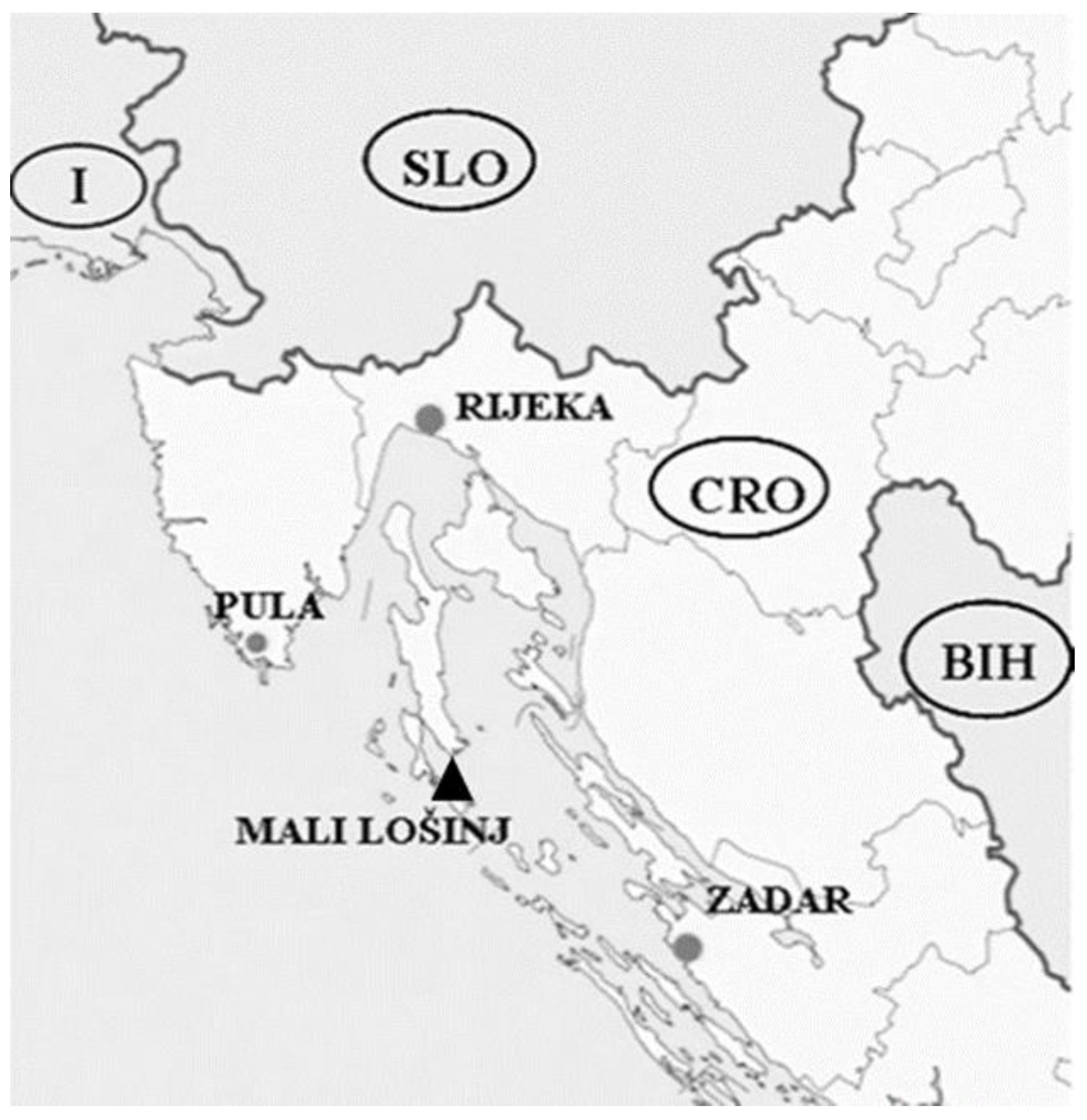
2.1. Sampling Site Description
2.2. Sampling and Analytical Method
2.2.1. Sampling
2.2.2. Desorption
2.2.3. Conditions of Analysis
2.2.4. Meteorological Parameters and Ozone Data
2.3. Data Analysis and Statistics
3. Results and Discussion
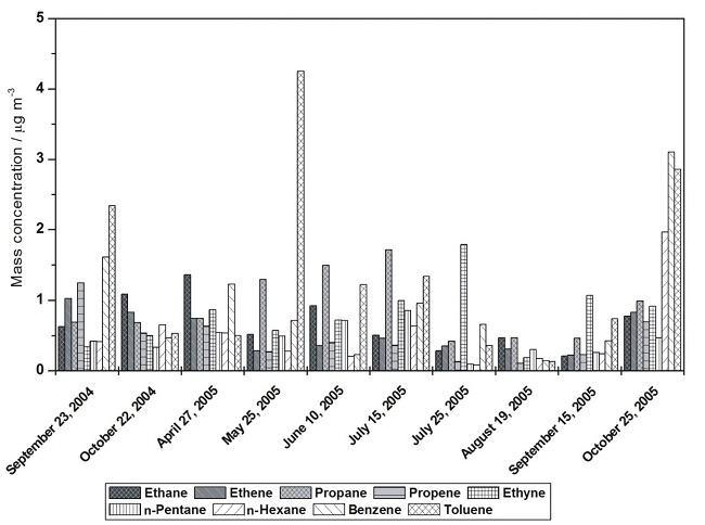
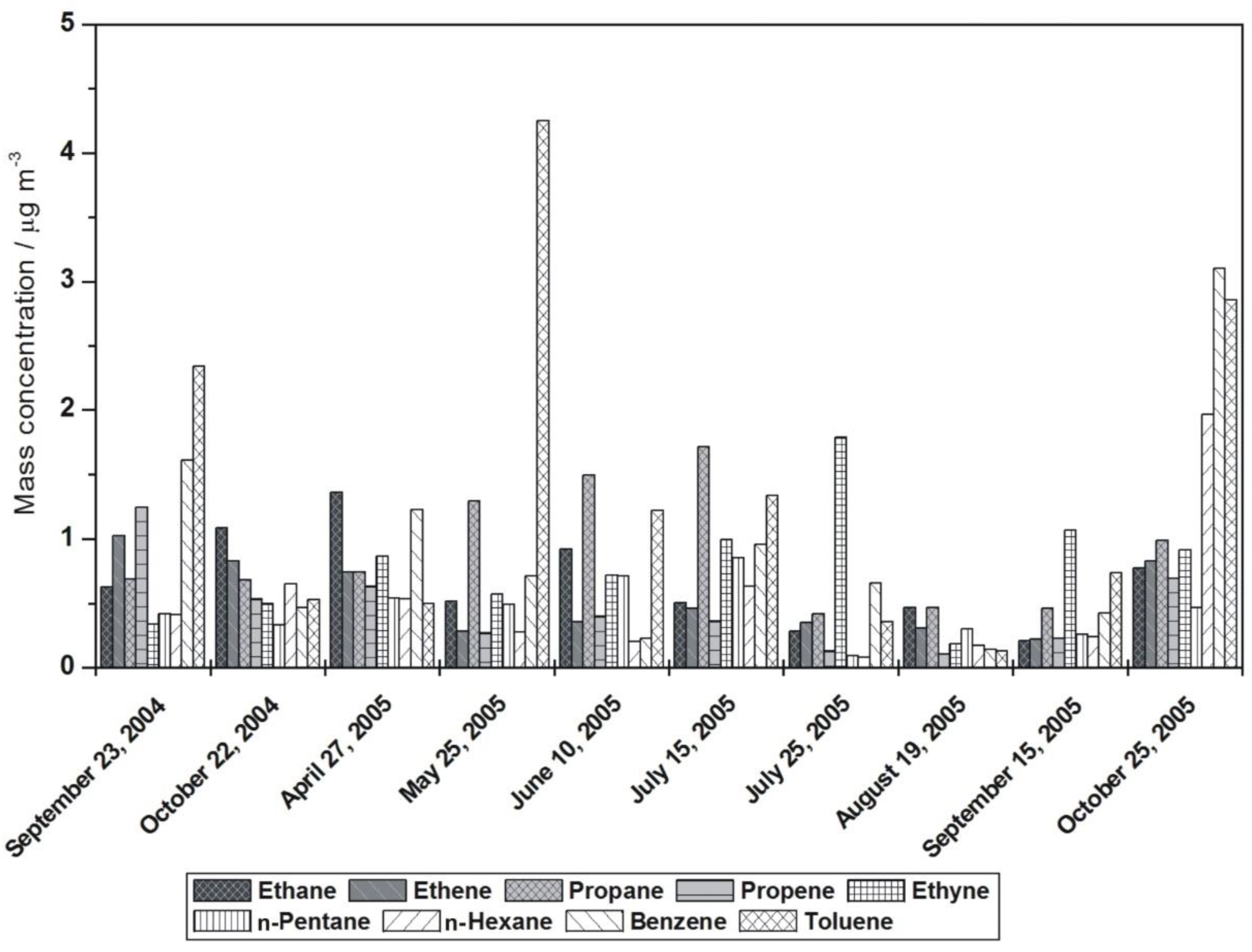
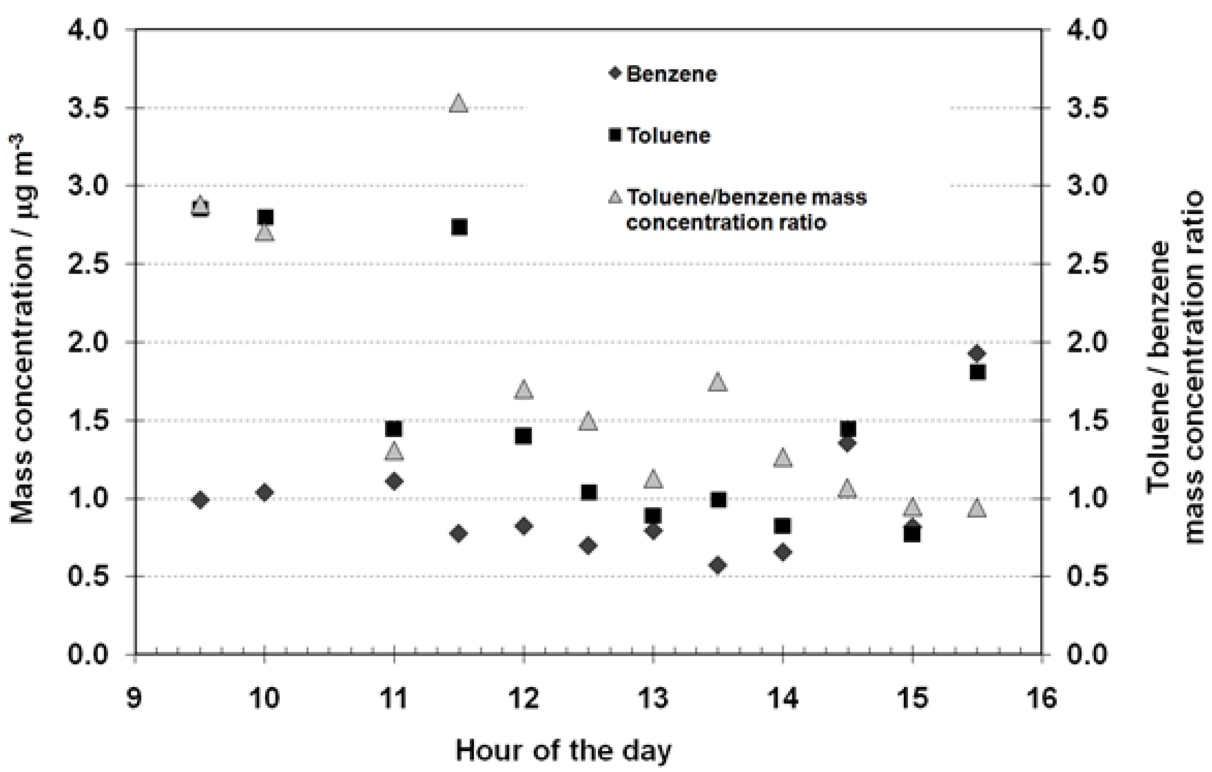
3.1. Volatile Hydrocarbon Mass Concentration in Ambient Air
3.2. Spearman’s Nonparametric Test
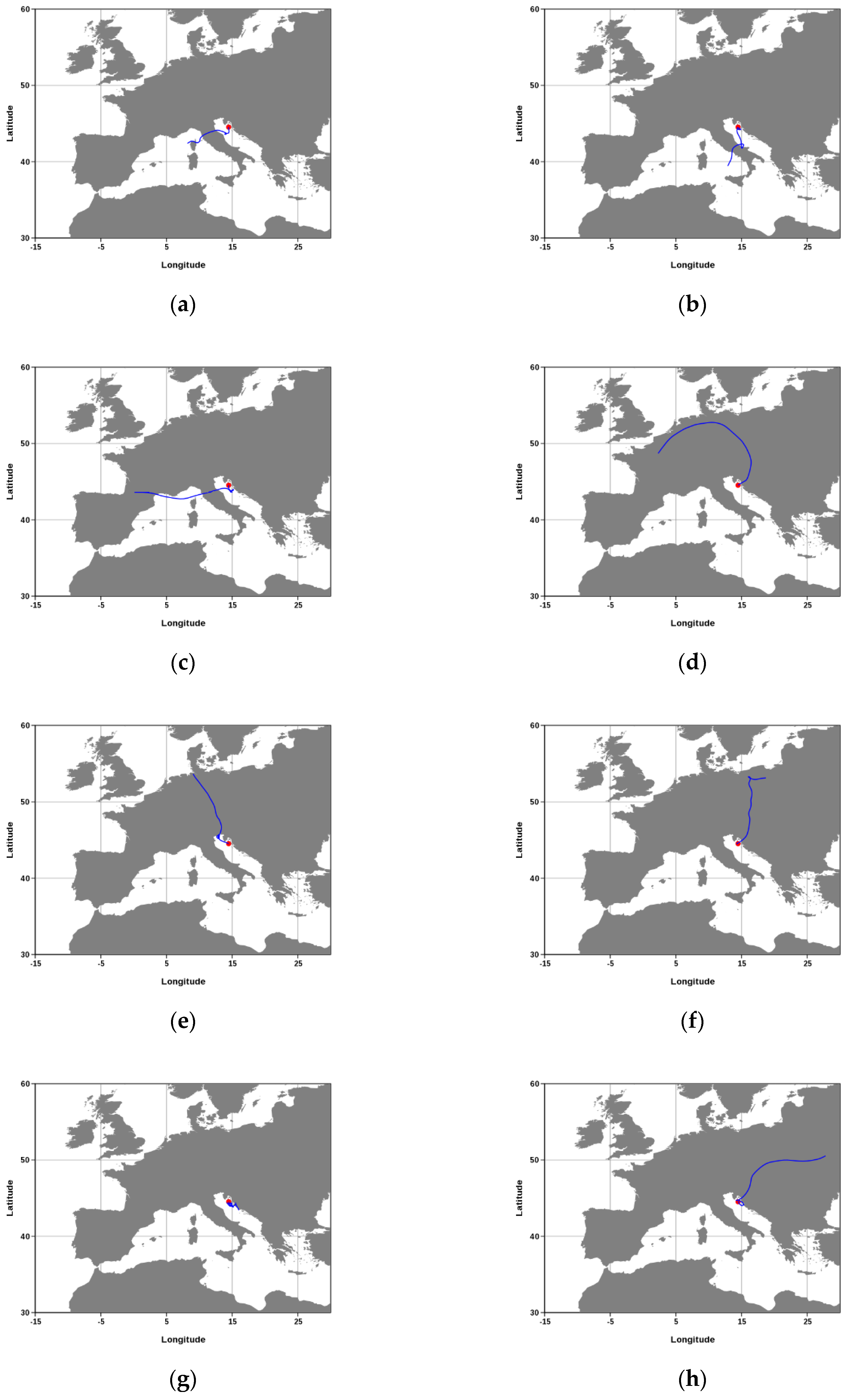
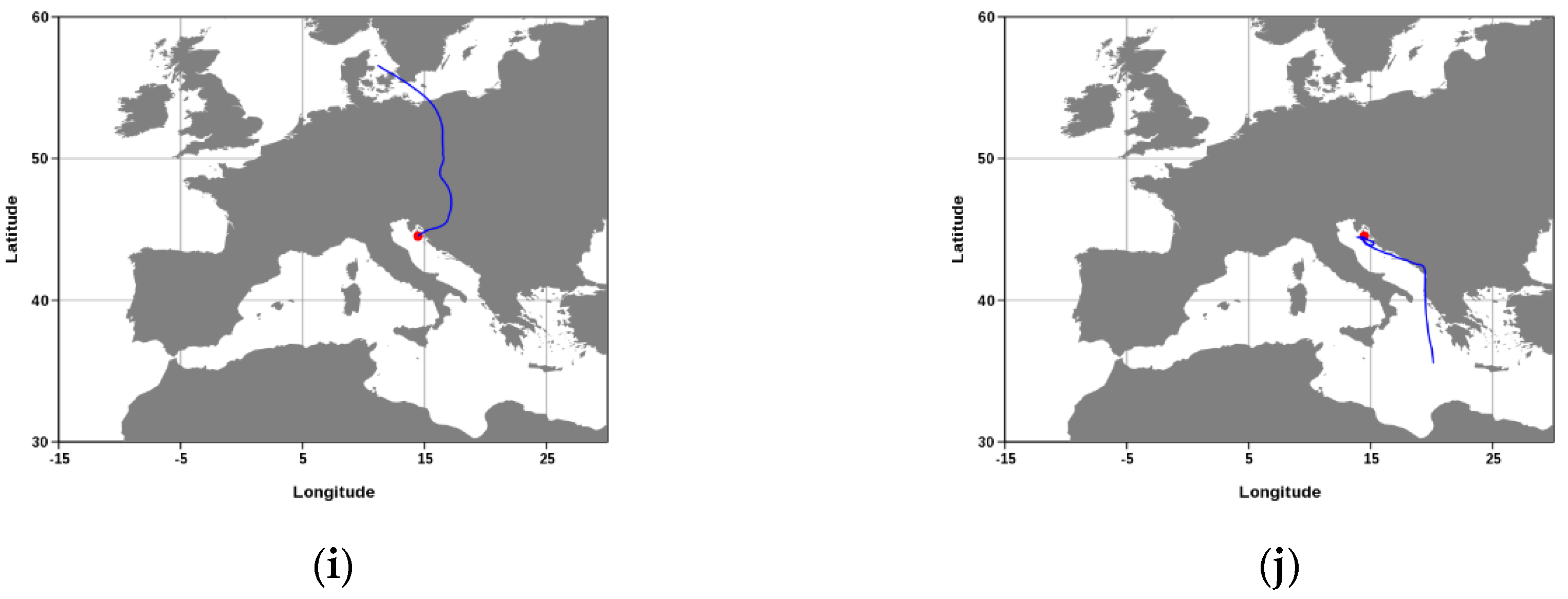
3.3. Air Trajectories
4. Conclusions
Author Contributions
Funding
Acknowledgments
Conflicts of Interest
References
- Mozaffar, A.; Zhang, Y.-L.; Fan, M.; Cao, F.; Lin, Y.-C. Characteristics of summertime ambient VOCs and their contributions to O3 and SOA formation in a suburban area of Nanjing, China. Atmos. Res. 2020, 240, 104923. [Google Scholar] [CrossRef]
- Tsilligianis, E.; Hammes, J.; Salvador, C.M.; Mentel, T.F.; Hallquist, M. Effect of NOx on 1,3,5-trimethylbenzene (TMB) oxidation product distribution and particle formation. Atmos. Chem. Phys. 2019, 19, 15073–15086. [Google Scholar] [CrossRef] [Green Version]
- Chetehouna, K. Volatile Organic Compounds: Emission, Pollution and Control; Nova Science Publishers, Inc.: Hauppauge, NY, USA, 2014; pp. 1–222. [Google Scholar]
- Ghirardo, A.; Lindstein, F.; Koch, K.; Buegger, F.; Schloter, M.; Albert, A.; Michelsen, A.; Winkler, J.B.; Schnitzler, J.-P.; Rinnan, R. Origin of volatile organic compound emissions from subarctic tundra under global warming. Glob. Chang. Biol. 2020, 26, 1908–1925. [Google Scholar] [CrossRef] [PubMed] [Green Version]
- Bakkenes, M.; Alkemade, J.R.M.; Ihle, F.; Leemans, R.; Latour, J.B. Assessing effects of forecasted climate change on the diversity and distribution of European higher plants for 2050. Glob. Chang. Biol. 2002, 8, 390–407. [Google Scholar] [CrossRef]
- Core Writing Team; Pachauri, R.K.; Reisinger, A. (Eds.) Climate Change 2007: Synthesis Report. Contribution of Working Groups I, II and III to the Fourth Assessment Report of the Intergovernmental Panel on Climate Change; IPCC: Geneva, Switzerland, 2008; p. 104. [Google Scholar]
- Keenan, T.; Niinemets, Ü.; Sabate, S.; Gracia, C.; Peñuelas, J. Seasonality of monoterpene emission potentials in Quercus ilex and Pinus pinea: Implications for regional VOC emissions modeling. J. Geophys. Res.-Atmos. 2009, 114, D22202. [Google Scholar] [CrossRef] [Green Version]
- Beniston, M.; Stephenson, D.; Christensen, O.; Ferro, C.T.; Frei, C.; Goyette, S.; Halsnaes, K.; Holt, T.; Jylhä, K.; Koffi, B.; et al. Future extreme events in European climate: An exploration of regional climate model projections. Clim. Chang. 2007, 81, 71–95. [Google Scholar] [CrossRef] [Green Version]
- Giorgi, F. Climate change hot-spots. Geophys. Res. Lett. 2006, 33, L08707. [Google Scholar] [CrossRef]
- Parry, M.L.; Canziani, O.F.; Palutikof, J.P.; van der Linden, P.J.; Hanson, C.E. (Eds.) Climate Change 2007: Impacts, Adaptation and Vulnerability. Contribution of Working Group II to the Fourth Assessment Report of the Intergovernmental Panel on Climate Change; Cambridge University Press: Cambridge, UK; New York, NY, USA, 2017; p. 976. [Google Scholar]
- Hertig, E.; Seubert, S.; Paxian, A.; Vogt, G.; Paeth, H.; Jacobeit, J. Changes of total versus extreme precipitation and dry periods until the end of the twenty-first century: Statistical assessments for the Mediterranean area. Theor. Appl. Climatol. 2013, 111, 1–20. [Google Scholar] [CrossRef]
- Peñuelas, J.; Filella, I.; Zhang, X.; Llorens, L.; Ogaya, R.; Lloret, F.; Comas, P.; Estiarte, M.; Terradas, J. Complex spatiotemporal phenological shifts as a response to rainfall changes. New Phytol. 2004, 161, 837–846. [Google Scholar] [CrossRef]
- Hartikainen, K.; Riikonen, J.; Nerg, A.M.; Kivimaenpaa, M.; Ahonen, V.; Tervahauta, A.; Karenlampi, S.; Maenpaa, M.; Rousi, M.; Kontunen-Soppela, S.; et al. Impact of elevated temperature and ozone on the emission of volatile organic compounds and gas exchange of silver birch (Betula pendula Roth). Environ. Exp. Bot. 2012, 84, 33–43. [Google Scholar] [CrossRef]
- Holopainen, J.K. Multiple functions of inducible plant volatiles. Trends Plant Sci. 2004, 9, 529–533. [Google Scholar] [CrossRef] [PubMed]
- Holopainen, J.K. Can forest trees compensate for stress-generated growth losses by induced production of volatile compounds? Tree Physiol. 2011, 31, 1356–1377. [Google Scholar] [CrossRef] [PubMed]
- Laothawornkitkul, J.; Taylor, J.E.; Paul, N.D.; Hewitt, C.N. Biogenic volatile organic compounds in the Earth system. New Phytol. 2009, 183, 27–51. [Google Scholar] [CrossRef] [PubMed]
- Cunningham, W.P.; Cunningham, M.A.; Saigo, B. Environmental Science: A Global Concern; McGraw-Hill Higher Education: New York, NY, USA, 2005; p. 600. [Google Scholar]
- Arsene, C.; Bougiatioti, A.; Mihalopoulos, N. Sources and variability of non-methane hydrocarbons in the Eastern Mediterranean. Glob. Nest J. 2009, 11, 333–340. [Google Scholar]
- Chan, C.Y.; Chan, L.Y.; Wang, X.M.; Liu, Y.M.; Lee, S.C.; Zou, S.C.; Sheng, G.Y.; Fu, J.M. Volatile organic compounds in roadside microenvironments of metropolitan Hong Kong. Atmos. Environ. 2002, 36, 2039–2047. [Google Scholar] [CrossRef]
- Warneke, C.; de Gouw, J.A.; Holloway, J.S.; Peischl, J.; Ryerson, T.B.; Atlas, E.; Blake, D.; Trainer, M.; Parrish, D.D. Multiyear trends in volatile organic compounds in Los Angeles, California: Five decades of decreasing emissions. J. Geophys. Res.-Atmos. 2012, 117, D00V17. [Google Scholar] [CrossRef]
- Alebić-Juretić, A.; Cvitaš, T.; Kezele, N.; Klasinc, L.; Pehnec, G.; Šorgo, G. Atmospheric particulate matter and ozone under heat-wave conditions: Do they cause an increase of mortality in Croatia? Bull. Environ. Contam. Tox. 2007, 79, 468–471. [Google Scholar] [CrossRef]
- Chen, H.; Goldberg, M.S.; Burnett, R.T.; Jerrett, M.; Wheeler, A.J.; Villeneuve, P.J. Long-Term Exposure to Traffic-Related Air Pollution and Cardiovascular Mortality. Epidemiology 2013, 24, 35–43. [Google Scholar] [CrossRef]
- Rückerl, R.; Schneider, A.; Breitner, S.; Cyrys, J.; Peters, A. Health effects of particulate air pollution: A review of epidemiological evidence. Inhal. Toxicol. 2011, 23, 555–592. [Google Scholar] [CrossRef]
- Stylianou, M.; Nicolich, M.J. Cumulative effects and threshold levels in air pollution mortality: Data analysis of nine large US cities using the NMMAPS dataset. Environ. Pollut. 2009, 157, 2216–2223. [Google Scholar] [CrossRef]
- Kumar, A.; Víden, I. Volatile Organic Compounds: Sampling Methods and Their Worldwide Profile in Ambient Air. Environ. Monit. Assess. 2007, 131, 301–321. [Google Scholar] [CrossRef] [PubMed]
- Ras, M.R.; Borrull, F.; Marcé, R.M. Sampling and preconcentration techniques for determination of volatile organic compounds in air samples. TRAC-Trend. Anal. Chem. 2009, 28, 347–361. [Google Scholar] [CrossRef]
- Palluau, F.; Mirabel, P.; Millet, M. Influence of relative humidity and ozone on the sampling of volatile organic compounds on Carbotrap/Carbosieve adsorbents. Environ. Monit. Assess. 2007, 127, 177–187. [Google Scholar] [CrossRef]
- Dettmer, K.; Engewald, W. Adsorbent materials commonly used in air analysis for adsorptive enrichment and thermal desorption of volatile organic compounds. Anal. Bioanal. Chem. 2002, 373, 490–500. [Google Scholar] [CrossRef] [PubMed]
- Ribes, A.; Carrera, G.; Gallego, E.; Roca, X.; Berenguer, M.J.; Guardino, X. Development and validation of a method for air-quality and nuisance odors monitoring of volatile organic compounds using multi-sorbent adsorption and gas chromatography/mass spectrometry thermal desorption system. J. Chromatogr. A 2007, 1140, 44–55. [Google Scholar] [CrossRef] [PubMed]
- Seco, R.; Peñuelas, J.; Filella, I.; Llusia, J.; Schallhart, S.; Metzger, A.; Müller, M.; Hansel, A. Volatile organic compounds in the Western Mediterranean Basin: Urban and rural winter measurements during the DAURE campaign. Atmos. Chem. Phys. Discuss. 2012, 12, 30909–30950. [Google Scholar] [CrossRef]
- Zeng, J.; Katsumoto, M.; Ide, R.; Inagaki, M.; Mukai, H.; Fujinuma, Y. Development of meteorological data explorer for Windows. In Data Analysis and Graphic Display Systems for Atmospheric Research Using PC; Fujinuma, Y., Ed.; CGER-M014-2003; Center for Global Environmental Research, NIES: Tsukuba, Japan, 2003; pp. 19–72. [Google Scholar]
- Zeng, J.; Tohjima, Y.; Fujinuma, Y.; Mukai, H.; Katsumoto, M. A study of trajectory quality using methane measurements from Hateruma Island. Atmos. Environ. 2003, 27, 1911–1919. [Google Scholar] [CrossRef]
- Tomikawa, Y.; Sato, K. Design of the NIPR trajectory model. Polar Meteorol. Glaciol. 2005, 19, 120–137. [Google Scholar]
- Hernández-Ceballos, M.Á.; Felice, L.D. Air mass trajectories to estimate the “most likely” areas to be affected by the release of hazardous materials in the atmosphere-feasibility study. Atmosphere 2019, 10, 253. [Google Scholar] [CrossRef] [Green Version]
- Prtenjak, M.T.; Belusic, D. Formation of reversed lee flow over the north-eastern Adriatic during bora. Geofizika 2009, 26, 145–155. [Google Scholar]
- Telišman Prtenjak, M.; Jeričević, A.; Bencetić Klaić, Z.; Alebić-Juretić, A.; Herceg Bulić, I. Atmospheric dynamics and elevated ozone concentrations in the northern Adriatic. Meteorol. Appl. 2013, 20, 482–496. [Google Scholar] [CrossRef]
- Baroja, O.; Goicolea, M.A.; Sampedro, M.C.; Rodriguez, E.; De Balugera, Z.G.; Alonso, A.; Barrio, R.J. Multisorbent tubes sampling used in thermal desorption cold trap injection with gas chromatography-mass spectrometry for C-2-C-6 hydrocarbon measurements in an urban atmosphere. Int. J. Environ. Anal. Chem. 2004, 84, 341–353. [Google Scholar] [CrossRef]
- Rothweiler, H.; Wager, P.A.; Schlatter, C. Comparison of tenax ta and carbotrap for sampling and analysis of volatile organic-compounds in air. Atmos. Environ. Part. B. Urban Atmos. 1991, 25, 231–235. [Google Scholar] [CrossRef]
- Faiola, C.L.; Erickson, M.H.; Fricaud, V.L.; Jobson, B.T.; VanReken, T.M. Quantification of biogenic volatile organic compounds with a flame ionization detector using the effective carbon number concept. Atmos. Meas. Tech. 2012, 5, 1911–1923. [Google Scholar] [CrossRef] [Green Version]
- Kállai, M.; Máté, V.; Balla, J. Effects of experimental conditions on the determination of the effective carbon number. Chromatographia 2003, 57, 639–644. [Google Scholar] [CrossRef]
- Scanlon, J.T.; Willis, D.E. Calculation of Flame Ionization Detector Relative Response Factors Using the Effective Carbon Number Concept. J. Chromatogr. Sci. 1985, 23, 333–340. [Google Scholar] [CrossRef]
- Tong, H.Y.; Karasek, F.W. Flame ionization detector response factors for compound classes in quantitative analysis of complex organic mixtures. Anal. Chem. 1984, 56, 2124–2128. [Google Scholar] [CrossRef]
- Durana, N.; Navazo, M.; Gomez, M.C.; Alonso, L.; Garcia, J.A.; Ilardia, J.L.; Gangoiti, G.; Iza, J. Long term hourly measurement of 62 non-methane hydrocarbons in an urban area: Main results and contribution of non-traffic sources. Atmos. Environ. 2006, 40, 2860–2872. [Google Scholar] [CrossRef]
- Filella, I.; Peñuelas, J. Daily, weekly, and seasonal time courses of VOC concentrations in a semi-urban area near Barcelona. Atmos. Environ. 2006, 40, 7752–7769. [Google Scholar] [CrossRef]
- Ho, K.F.; Lee, S.C.; Guo, H.; Tsai, W.Y. Seasonal and diurnal variations of volatile organic compounds (VOCs) in the atmosphere of Hong Kong. Sci. Total Environ. 2004, 322, 155–166. [Google Scholar] [CrossRef]
- Helmig, D.; Thomspon, C.R.; Evans, J.; Boylan, P.; Hueber, J.; Park, J.-H. Highly elevated atmospheric levels of volatile organic compounds in the uintah basin, Utah. Environ. Sci. Tech. 2014, 48, 4707–4715. [Google Scholar] [CrossRef] [PubMed]
- Kelessis, A.G.; Petrakakis, M.J.; Zoumakis, N.M. Determination of benzene, toluene, ethylbenzene, and xylenes in urban air of Thessaloniki, Greece. Environ. Toxicol. 2006, 21, 440–443. [Google Scholar] [CrossRef] [PubMed]
- Miri, M.; Aghdam Shendi, M.R.; Reza Ghaffari, H.; Ebrahimi Aval, H.; Ahmadi, E.; Taban, E.; Gholizadeh, A.; Yazdani Aval, M.; Mohammadi, A.; Azari, A. Investigation of outdoor BTEX: Concentration, variations, sources, spatial distribution, and risk assessment. Chemosphere 2016, 163, 601–609. [Google Scholar] [CrossRef] [PubMed]
- Baudic, A.; Gros, V.; Sauvage, S.; Locoge, N.; Sanchez, O.; Sarda-Estève, R.; Kalogridis, C.; Petit, J.-E.; Bonnaire, N.; Baisnée, D.; et al. Seasonal variability and source apportionment of volatile organic compounds (VOCs) in the Paris megacity (France). Atmos. Chem. Phys. 2016, 16, 11961–11989. [Google Scholar] [CrossRef] [Green Version]
- Heiden, A.C.; Kobel, K.; Komenda, M.; Koppmann, R.; Shao, M.; Wildt, J. Toluene emissions from plants. Geophys. Res. Lett. 1999, 26, 1283–1286. [Google Scholar] [CrossRef] [Green Version]
- Kim, S.; Karl, T.; Guenther, A.; Tyndall, G.; Orlando, J.; Harley, P.; Rasmussen, R.; Apel, E. Emissions and ambient distributions of Biogenic Volatile Organic Compounds (BVOC) in a ponderosa pine ecosystem: Interpretation of PTR-MS mass spectra. Atmos. Chem. Phys. 2010, 10, 1759–1771. [Google Scholar] [CrossRef] [Green Version]
- Russo, R.S.; Zhou, Y.; White, M.L.; Mao, H.; Talbot, R.; Sive, B.C. Multi-year (2004–2008) record of nonmethane hydrocarbons and halocarbons in New England: Seasonal variations and regional sources. Atmos. Chem. Phys. 2010, 10, 4909–4929. [Google Scholar] [CrossRef] [Green Version]
- White, M.L.; Russo, R.S.; Zhou, Y.; Ambrose, J.L.; Haase, K.; Frinak, E.K.; Varner, R.K.; Wingenter, O.W.; Mao, H.; Talbot, R.; et al. Are biogenic emissions a significant source of summertime atmospheric toluene in the rural Northeastern United States? Atmos. Chem. Phys. 2009, 9, 81–92. [Google Scholar] [CrossRef] [Green Version]
- Atkinson, R.; Arey, J. Atmospheric Degradation of Volatile Organic Compounds. Chem. Rev. 2003, 103, 4605–4638. [Google Scholar] [CrossRef]
- Kovač-Andrić, E.; Gvozdić, V.; Herjavić, G.; Muharemović, H. Assessment of ozone variations and meteorological influences in a tourist and health resort area on the island of Mali Lošinj (Croatia). Environ. Sci. Pollut. R. 2013, 20, 5106–5113. [Google Scholar] [CrossRef] [Green Version]
- Alebić-Juretić, A.; Čanić, K.S.; Kavčič, I.; Klaić, Z.B. H15-12: The Saharan Sand episode on 12th of April 2002 in the Northern Adriatic Area, Croatia. In Proceedings of the 15th International Conference on Harmonisation within Atmospheric Dispersion Modelling for Regulatory Purposes, Madrid, Spain, 6–9 May 2013. [Google Scholar]
- Žabkar, R.; Rakovec, J.; Gaberšek, S. A trajectory analysis of summertime ozone pollution in Slovenia. Geofizika 2008, 25, 179–202. [Google Scholar]


| 23 September 2004 | 22 October 2004 | 27 April 2005 | 25 May 2005 | 10 June 2005 | 15 July 2005 | 25 July 2005 | 19 August 2005 | 15 September 2005 | 25 October 2005 | |
|---|---|---|---|---|---|---|---|---|---|---|
| Ethane | 0.6 ± 0.4 | 1.1 ± 0.8 | 1.4 ± 0.3 | 0.5 ± 0.2 | 0.9 ± 0.1 | 0.5 ± 0.3 | 0.3 ± 0.1 | 0.47± 0.08 | 0.21 ± 0.03 | 0.8 ± 0.4 |
| Ethene | 1.0 ± 0.2 | 0.8 ± 0.1 | 0.8 ± 0.4 | 0.3 ± 0.1 | 0.4 ± 0.1 | 0.5 ± 0.4 | 0.4 ± 0.2 | 0.31 ± 0.06 | 0.22 ± 0.08 | 0.8 ± 0.6 |
| Propane | 0.7 ± 0.3 | 0.7 ± 0.2 | 0.8 ± 0.2 | 1 ± 1 | 1.5 ± 0.8 | 1.7 ± 0.8 | 0.4 ± 0.2 | 0.5 ± 0.2 | 0.5 ± 0.1 | 1.0 ± 0.2 |
| Propene | 1.3 ± 0.3 | 0.6 ± 0.1 | 0.6 ± 0.2 | 0.27 ± 0.09 | 0.4 ± 0.2 | 0.4 ± 0.6 | 0.13 ± 0.02 | 0.11 ± 0.03 | 0.23 ± 0.04 | 0.7 ± 0.2 |
| Ethyne | 0.34 ± 0.05 | 0.5 ± 0.1 | 0.9 ± 0.1 | 0.6 ± 0.3 | 0.7 ± 0.2 | 1.0 ± 0.2 | 1.8 ± 0.1 | 0.19 ± 0.06 | 1.1 ± 0.1 | 0.9 ± 0.4 |
| n-Butane | 0.3 ± 0.1 | 0.7 ± 0.3 | 0.6 ± 0.4 | 1.1 ± 0.9 | 1.3 ± 0.5 | 1.1 ± 0.7 | 0.5 ± 0.3 | 0.4 ± 0.1 | 0.62 ± 0.09 | |
| But-1-ene | 0.49 ± 0.08 | 0.9 ± 0.1 | 0.5 ± 0.4 | 0.2 ± 0.1 | 0.1 ± 0.1 | 0.22 ± 0.06 | 0.2 ± 0.2 | 0.3 ± 0.1 | ||
| Propyne | 0.76± 0.07 | 0.60 ± 0.07 | 0.39 ± 0.06 | 0.3 ± 0.1 | 0.20 ± 0.04 | 0.5 ± 0.3 | 0.13 ± 0.04 | 1.5 ± 0.2 | ||
| But-1-yne | 0.27 ± 0.05 | 0.29 ± 0.05 | ||||||||
| Cis-2-pentene | 0.4 ± 0.1 | 0.15 ± 0.05 | ||||||||
| n-Pentane | 0.4 ± 0.3 | 0.3 ± 0.5 | 0.5 ± 0.3 | 0.5 ± 0.3 | 0.7 ± 0.3 | 1 ± 1 | 0.09 ± 0.03 | 0.3 ± 0.2 | 0.3 ± 0.1 | 0.5 ± 0.1 |
| Pent-1-ene | 0.3 ± 0.1 | 0.4 ± 0.2 | 0.3 ± 0.2 | 0.4 ± 0.2 | 0.11 ± 0.08 | |||||
| n-Hexane | 0.4 ± 0.1 | 0.7 ± 0.9 | 0.5 ± 0.1 | 0.3 ± 0.2 | 0.20 ± 0.09 | 0.6 ± 0.2 | 0.08 ± 0.02 | 0.2 ± 0.1 | 0.24 ± 0.08 | 2 ± 1 |
| Hex-1-ene | 0.4 ± 0.8 | 0.16 | 0.2 ± 0.1 | 0.07 ± 0.01 | 0.13 ± 0.08 | |||||
| Methylcyclopentane | 0.26 ± 0.01 | 0.31 ± 0.02 | ||||||||
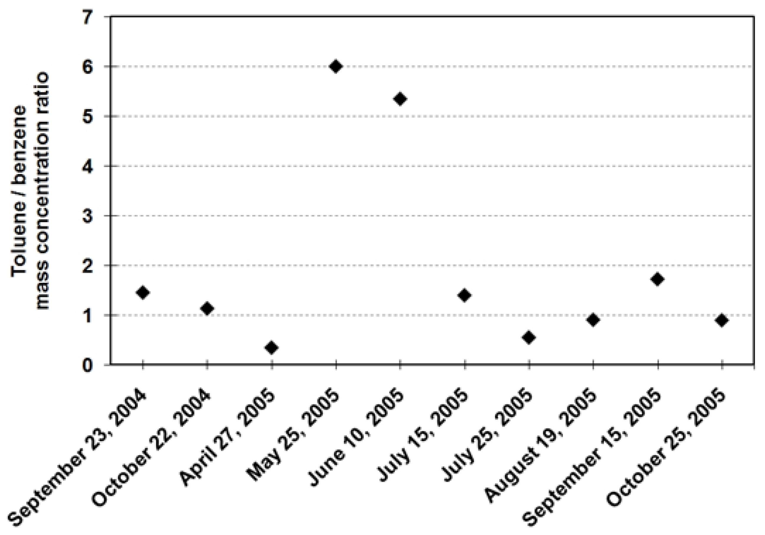
| Benzene | 1.6 ± 0.1 | 0.5 ± 0.1 | 1.2 ± 0.3 | 0.7 ± 0.1 | 0.2 ± 0.2 | 1.0 ± 0.1 | 0.6 ± 0.2 | 0.1 ± 0.1 | 0.4 ± 0.2 | 3.1 ± 0.5 |
| 2,4-Dimethylpentane | 0.6 ± 0.1 | 1.4 ± 0.1 | ||||||||
| Cyclohexane | 0.3 ± 0.1 | 1.2 ± 0.1 | ||||||||
| 2,3-Dimethylpentane | 1.45 ± 0.06 | |||||||||
| 2-Methylhexane | 0.34 ± 0.03 | |||||||||
| 3-Methylhexane | 1.9 ± 0.1 | 1.7 ± 0.2 | ||||||||
| n-Heptane | 0.9 ± 0.3 | 1 ± 1 | 0.3 ± 0.1 | |||||||
| 2,2,4-Trimethylpentane | 0.4 ± 0.3 | 0.7 ± 0.3 | ||||||||
| Methylcyclohexane | 0.5 ± 0.2 | |||||||||
| Toluene | 2.3 ± 0.3 | 0.5 ± 0.3 | 0.5 ± 0.4 | 4 ± 1 | 1.2 ± 0.7 | 1.3 ± 0.3 | 0.3 ± 0.3 | 0.1 ± 0.2 | 0.7 ± 0.1 | 2.9 ± 0.8 |
| Ethane | Ethene | Propane | Propene | Ethyne | n-Butane | n-Pentane | n-Hexane | Benzene | Toluene | Temperature | Solar radiation | Ozone | |
|---|---|---|---|---|---|---|---|---|---|---|---|---|---|
| Ethane | 1 | 0.52 | 0.67 | 0.34 | 0.62 | 0.24 | 0.46 | 0.32 | 0.41 | 0.40 | −0.57 | −0.61 | −0.02 |
| Ethene | 1 | 0.29 | 0.10 | 0.34 | −0.08 | 0.16 | 0.25 | 0.51 | 0.14 | −0.12 | −0.38 | −0.02 | |
| Propane | 1 | 0.38 | 0.75 | 0.64 | 0.70 | 0.46 | 0.33 | 0.65 | −0.39 | −0.36 | 0.03 | ||
| Propene | 1 | 0.37 | 0.31 | 0.20 | 0.29 | −0.09 | 0.38 | −0.69 | −0.50 | −0.64 | |||
| Ethyne | 1 | 0.38 | 0.43 | 0.22 | 0.23 | 0.50 | −0.46 | −0.45 | 0.05 | ||||
| n-Butane | 1 | 0.65 | 0.31 | −0.10 | 0.47 | −0.23 | −0.04 | −0.16 | |||||
| n-Pentane | 1 | 0.58 | 0.32 | 0.65 | −0.26 | −0.26 | 0.04 | ||||||
| n-Hexane | 1 | 0.58 | 0.81 | −0.30 | −0.44 | −0.29 | |||||||
| Benzene | 1 | 0.52 | −0.14 | −0.58 | 0.00 | ||||||||
| Toluene | 1 | −0.51 | −0.60 | −0.27 | |||||||||
| Temperature | 1 | 0.70 | 0.52 | ||||||||||
| Solar Radiation | 1 | 0.50 | |||||||||||
| Ozone | 1 |
© 2020 by the authors. Licensee MDPI, Basel, Switzerland. This article is an open access article distributed under the terms and conditions of the Creative Commons Attribution (CC BY) license (http://creativecommons.org/licenses/by/4.0/).
Share and Cite
Herjavić, G.; Matasović, B.; Arh, G.; Kovač-Andrić, E. Investigation of Non-Methane Hydrocarbons at a Central Adriatic Marine Site Mali Lošinj, Croatia. Atmosphere 2020, 11, 651. https://doi.org/10.3390/atmos11060651
Herjavić G, Matasović B, Arh G, Kovač-Andrić E. Investigation of Non-Methane Hydrocarbons at a Central Adriatic Marine Site Mali Lošinj, Croatia. Atmosphere. 2020; 11(6):651. https://doi.org/10.3390/atmos11060651
Chicago/Turabian StyleHerjavić, Glenda, Brunislav Matasović, Gregor Arh, and Elvira Kovač-Andrić. 2020. "Investigation of Non-Methane Hydrocarbons at a Central Adriatic Marine Site Mali Lošinj, Croatia" Atmosphere 11, no. 6: 651. https://doi.org/10.3390/atmos11060651