Simulation of Wind Speed Based on Different Driving Datasets and Parameterization Schemes Near Dunhuang Wind Farms in Northwest of China

Abstract

In this study, we evaluate the impacts of different datasets (e.g., NCEP global forecast system (GFS) and ERA5) that are used to derive the initial and boundary conditions, various planetary parameterization boundary layer (PBL) schemes and radiation parameterization schemes on wind speed simulations over wind farms near Dunhuang in Northwest of China. The mesoscale community Weather Research and Forecasting (WRF) model is employed to simulate the wind speeds in March of 2014. The sensitivity of numerical simulations to different PBL schemes, including the Yonsei University (YSU), the Asymmetric Convective Model (ACM2) and the Mellor–Yamada–Janjic (MYJ) scheme are examined. Besides, simulations with different radiation parameterization schemes, including the Rapid Radiative Transfer Model for general circulation model (GCM) applications (RRTMG) and the Fu–Liou–Gu radiative transfer scheme (FLG), are compared. Based on hourly observation data from three national basic meteorological observing stations and an anemometer tower in Dunhuang, the simulation results are evaluated. Results show that, using the GFS data as the initial data, the simulation error of 10-m wind speed is rather smaller under the combination of the YSU and FLG. When using the ERA5 data as the initial data, the error of the 2-m temperature simulation is smaller, and it is also less than that of the 10-m wind speed simulation. The simulation results show significant differences at different altitudes. The relative error of wind speed is larger at higher altitude. In the vertical direction, the wind speed is smaller at a lower height and so is the simulation error. In terms of wind speed from the anemometer tower, the error of the wind speed is related to the magnitude of the observed wind speed. Therefore, according to specific conditions of the simulated area, selecting an appropriate combination of initial data and parameterization schemes can effectively reduce the errors of simulated wind speed.

1. Introduction

The correct assessment and prediction of wind energy resources are important for both the siting of wind farms and the power-generation process. Accurate prediction of wind speed (WS) is conducive to timely adjustment of the power system dispatching, reducing associated operating costs, thus, effectively improving the efficiency of power generation [1]. The methods for the short-term forecast of WS in wind farms in the world mainly include statistical forecast, the downscaling method in numerical simulation, ensemble forecast [2,3,4,5,6]. With the development of mesoscale numerical models, the forecasting, exploitation and utilization of wind energy resources through numerical models has received worldwide attention [7,8]. Wind energy resources in Jiuquan have been simulated by using the Weather Research and Forecasting (WRF) model, and it is found that the WS and wind energy density are largest in winter and relatively smaller in summer [1]. The WRF has also been used to predict the WS of wind turbines at different heights, and results show that the prediction effect is largely influenced by the terrain [9].

The WRF model is widely used in simulating the potential wind energy production and WS [10,11,12], but the simulation results are affected by many factors. A year of simulation and evaluation have been conducted in the northwest region of China, and results show that the terrain and underlying surface have a large impact on the simulated WS, temperature, and precipitation. The simulation errors are closely correlated with the underlying surface conditions, especially for numerical simulations less influenced by the weather background in regions with complex terrain [13]. In the simulation, the parameterization schemes of the parameterization boundary layer (PBL) and radiation also have a significant influence on the forecast accuracy of the WS [14]. Through a simulation study of the gale process in Xinjiang, it is concluded that the impact of PBL parameterization schemes on the simulation is mainly influenced by the vertical mixing processing algorithm, and different parameterization schemes are affected by the terrain to a different extent [15]. Simulations in the western Inner Mongolia region by the WRF model show that different boundary layer parameterization schemes have their own advantages for simulating WSs at different heights [9]. Besides, changes in radiative heating data affect the atmospheric circulation and the thermal condition of the underlying surface, which further influences the PBL process, and thus the uncertainty of simulation results increases. The radiation parameterization schemes also affect the cumulus convective process and the land surface processes. The radiation parameterization scheme can influence the heating efficiency of the atmosphere, the energy in the near-surface layer, and change the pressure difference, thus influencing the simulation of WS [16]. Therefore, a reasonable combination of parameterization schemes based on the altitude, underlying surface, in the specific areas can effectively improve the ability of numerical models to simulate local wind energy and reduce the uncertainty of simulation [17].

In addition to the parameterization schemes, the simulation ability of the WRF varies significantly with different initial data. A comparative study shows that the WRF model performs better on the WS forecast with the global forecast system (GFS) as the initial data than with the data from the Japan Meteorological Agency [18]. With the initial data provided by the ERA-Interim and FNL data for driving the WRF model, results show that the two initial data differ considerably at the sub-synoptic scale, thus resulting in different simulation results [8]. The influence of initial data on the numerical model also differs over different integration periods.

The wind speed near Dunhuang is relatively high, which has great potential for wind energy development. Numerical simulations are necessary for wind farm siting and wind power forecasting in the Dunhuang area with complex terrain. Although short-term forecasts of wind power with high spatial-temporal resolution can be obtained through the WRF model [19,20], there are significant regional differences for the forecast of WS, which is relatively poor in some regions such as mountainous areas [19]. Therefore, it is necessary to evaluate the parameterization schemes and coordinate system for the application of the WRF model in regions nearby Dunhuang, where the underlying surface is rather complex, aiming to find a combination of parameterization schemes suitable for this area. On this basis, a large number of exploratory studies could also be conducted, which helps to reduce the forecast errors of the model, thus improving the performance of WS simulation. In this paper, hourly observations from the Dunhuang station and nearby national basic meteorological observing station, and WS observations of different heights from the anemometer tower are adopted. Simulation results of the WRF model are evaluated under different combinations of initial data (GFS and ERA5), PBL parameterization schemes (Asymmetric Convective Model (ACM2), Mellor–Yamada–Janjic (MYJ), and Yonsei University (YSU)), and radiation parameterization schemes (Rapid Radiative Transfer Model (RRTMG) and Fu–Liou–Gu radiative transfer scheme (FLG)), aiming to provide a reference for a more accurate simulation of wind speed over complex terrain in the Dunhuang area.

2. Experiment Design

The WRF-ARW Version 3.8.1 model is used in this study. WRF is a fully compressible non-hydrostatic model with a horizontal lattice Arakawa-C format, a vertical coordinate system of power quality, and a Euler center based on terrain following. Physical parameterization schemes can be selected in the model, including microphysics, cumulus, planetary boundary layer, and land surface processes.

Based on the results of numerical simulations for temperature, WS, precipitation in northwest China, and well-established settings, including the simulation domains, and vertical resolution (with the center point at 40°36’ N, 96°24’ E) are adopted in this study [12]. The settings of the nested domain are shown in

Table 1. Parameters of nested domain.

Domains	Grid Points	Resolution/km
1	236 × 162	9
2	223 × 169	3
3	382 × 202	1

. It is vertically divided into 55 layers with 50 hPa at the top. The microphysical process is the WMS6 scheme, the physical scheme in the surface layer is the Monin–Obukhov scheme, the land surface process is the Noah scheme, and the cumulus convection scheme is the Kain–Fritsch (new Eta) scheme (D01 and D02, there is no cumulus parameterization in D03). Two initial data (GFS and ERA5), three PBL parameterization schemes (ACM2, MYJ, and YSU), and two radiation parameterization schemes (RRTMG and FLG) are used for model simulations, respectively (

Table 2. Parameterization schemes of numerical simulation.

Exp.	S1	S2	S3	S4	S5	S6
Schemes	ACM2 + FLG	ACM2 + RRTMG	MYJ + FLG	MYJ + RRTMG	YSU + FLG	YSU + RRTMG

). The simulation results (D03) are interpolated to the three stations (Figure 1b) by using the nearest neighbor interpolation and further evaluated by using the observations from three observing stations. The three national basic meteorological observing stations (Figure 1b) are Dunhuang station (40°9’ N, 94°41’ E, altitude 1139.00 m), and two stations near Dunhuang—Anxi station (40°32’ N, 95°47’ E, with the altitude of 1170.90 m), and Hongliuhe station (41°32’ N, 94°40’ E, altitude 1573.80 m).

3. Data

The data used in this study include the ERA5 reanalysis data from the European Centre for Medium-Range Weather Forecasts (ECMWF), the GFS data from the National Centers for Environmental Prediction (NCEP), national basic meteorological observations, and observation data of the anemometer tower.

ERA5 is the fourth-generation global atmospheric reanalysis data developed and issued by ECMWF, which is obtained by the Integrated Forecasting System (IFS) from ECMWF by assimilating conventional surface and atmospheric meteorological observation data and satellite remote sensing data to the model. It is one of the most technologically advanced reanalysis datasets available to date. The hourly observation data from three stations (Figure 1b) in March 2014 are adopted in the study. Meteorological elements used in this paper include the hourly observed 10-m WS and 2-m temperature (T2).The anemometer tower data, including WS data at the heights of 10 m, 30 m, 60 m, are obtained from a wind farm in Gansu (96°50’ E, 40°65’ N, altitude 1416.00 m). The monthly average WS of anemometer tower data ranges from 4.2 to 6.7 m∙s⁻¹ during the observation period from January to December, with the highest WS in May and the smallest in December, and the annual average WS is 5.4 m∙s⁻¹. The dominant wind direction (WD) at the height of 10 m at the wind farm is the easterly northeast wind, with the wind of northeast, easterly northeast and east direction occurring most frequently at rates of 19.5%, 16.4% and 11.7%, respectively. The WD is easterly at 30 m and 60 m, which is the same as the 10-m WD.

4. Results

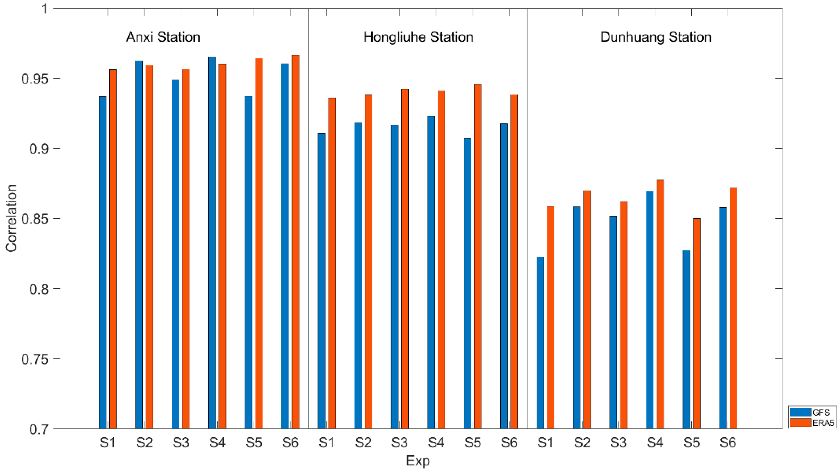
4.1. Correlation Coefficients for WS

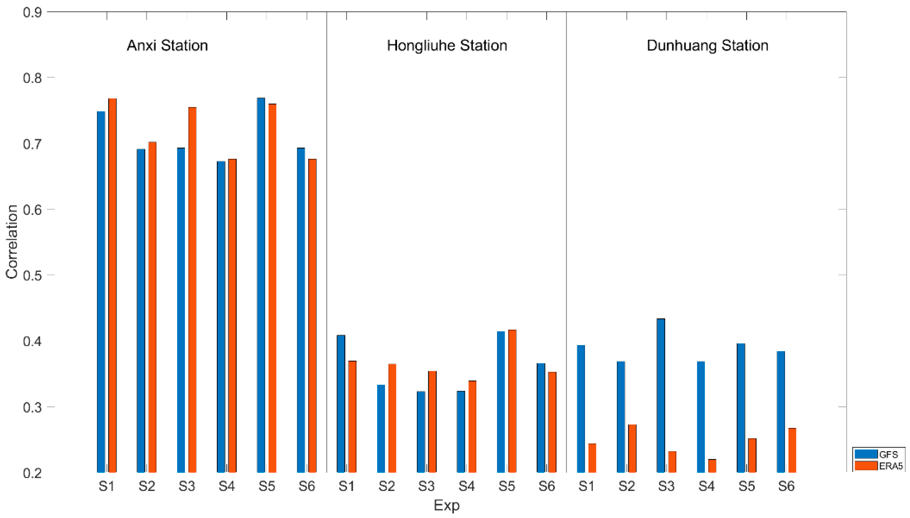
The correlation coefficient (R) gives a more accurate representation of the degree and direction of correlation between simulations and observations. Figure 2 shows the correlation coefficients (Rs) between simulated and observed 10-m WS at three stations under the combinations of different initial data and different parameterization schemes. It shows that the R at Anxi station is the highest, mostly around 0.7. When the ERA5 data are used as the initial data, the R is higher than that with the GFS, but there is no significant difference between the two datasets. According to the comparison of different combinations of PBL schemes and radiation schemes, the R of the S5 is the highest, which is close to 0.8. Meanwhile, the R of the S4 is the lowest, which is below 0.7. The Rs at Hongliuhe station are much smaller than those at Anxi station, mostly around 0.4. There is no significant difference between the simulation results with two different initial data at Hongliuhe station. The R of S5 is the highest at Hongliuhe station, which is similar to that at Anxi station, reaching above 0.4. Different from the other two stations, the Rs with the GFS and ERA5 at Dunhuang station are significantly different, with the Rs being significantly higher in the GFS than the ERA5. The Rs are around 0.4 with the GFS as the initial data, which are all below 0.3 with the ERA5. The Rs with the GFS as the initial data indicate that higher R can be obtained by the S3 scheme. It should be noted that the correlation coefficients for Hongliue and Dunhuang station are very small, which is worth discussing further.

The average Rs at three stations (

Table 3. Average correlation coefficients (Rs) of different combinations of initial data and parameterization schemes.

R	S1	S2	S3	S4	S5	S6
GFS	0.52 *	0.46 *	0.48 *	0.46 *	0.53 *	0.48 *
ERA5	0.46 *	0.45 *	0.45 *	0.41 *	0.48 *	0.43 *

Note: * trend significant at a = 0.01.

) show that the Rs (around 0.5) with the GFS as initial data are overall higher than those (around 0.45) with the ERA5. The comparison of Rs under different combinations of parameterization schemes exhibits that S5 owes the highest R. The highest Rs are 0.53 and 0.48 for the GFS and ERA5 as initial data, respectively. Meanwhile, the R in the S4 is the smallest. The Rs for all simulation results reaches the 0.01 significance level.

4.2. Error Percentage of WS

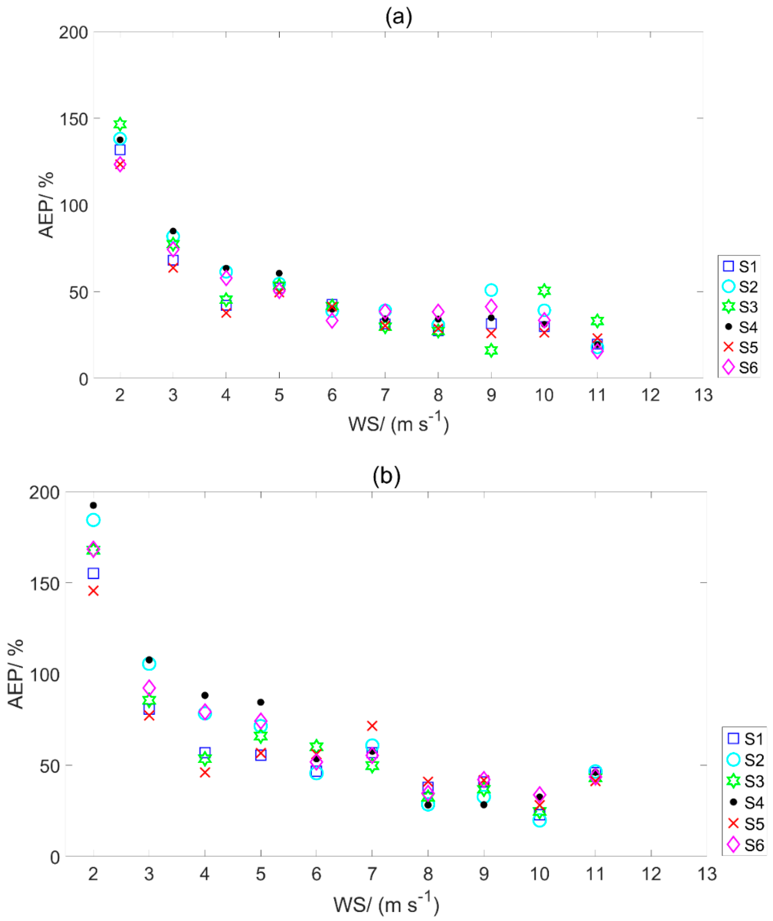
Besides the correlations, the average absolute error percentage (AEP) can also be used to quantitatively evaluate the simulation results. To further compare the AEP of different simulations, comparative evaluations are also performed for WS at different scales.

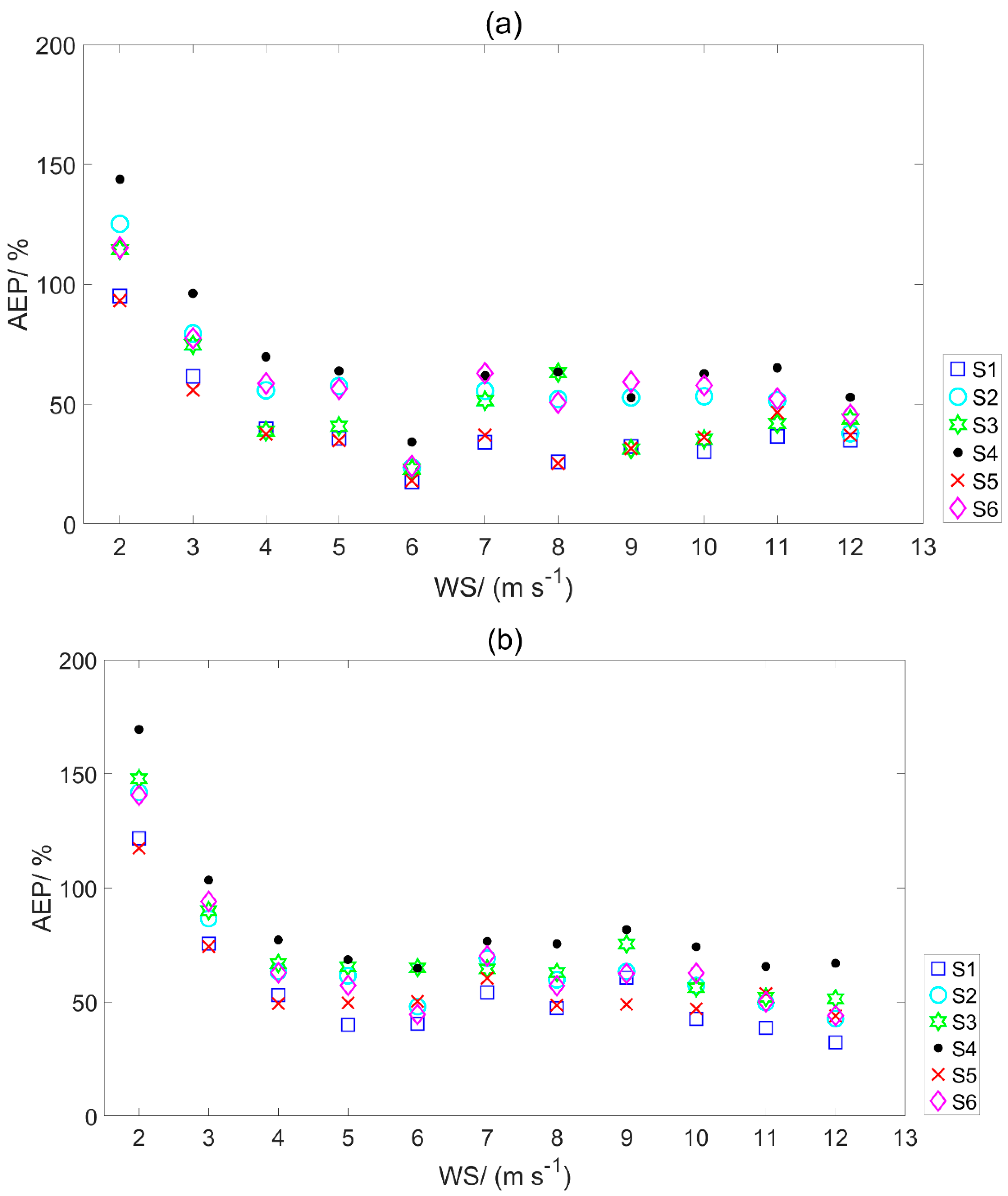
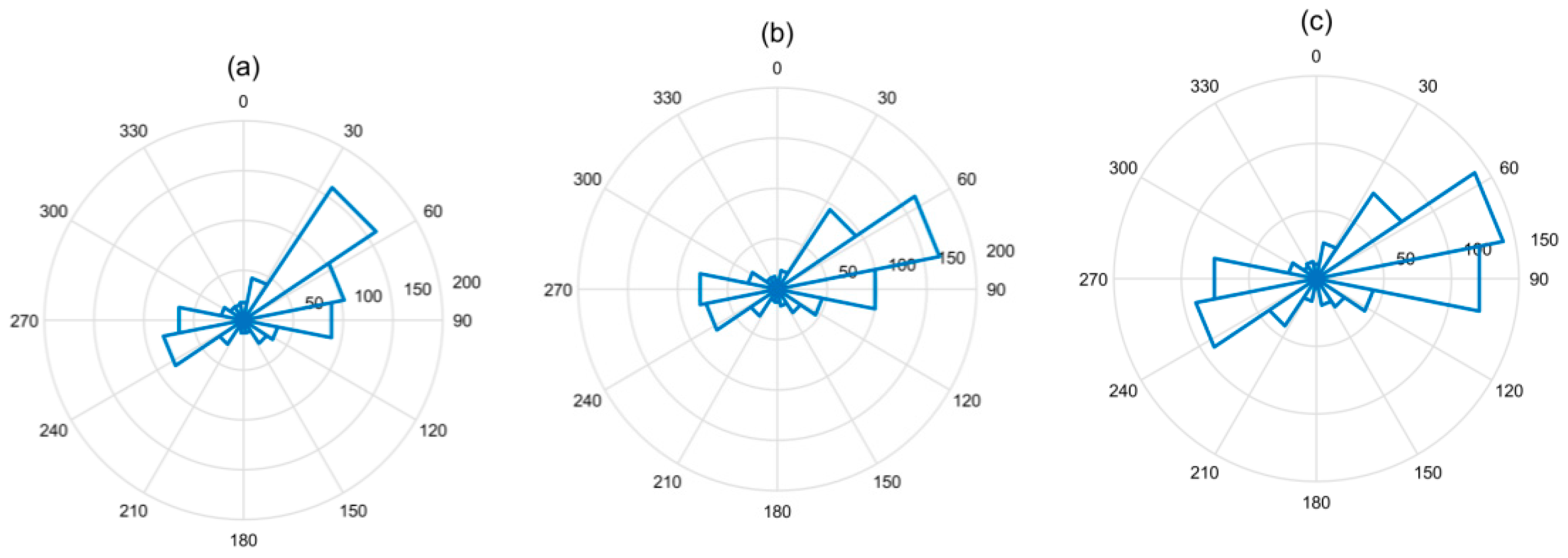
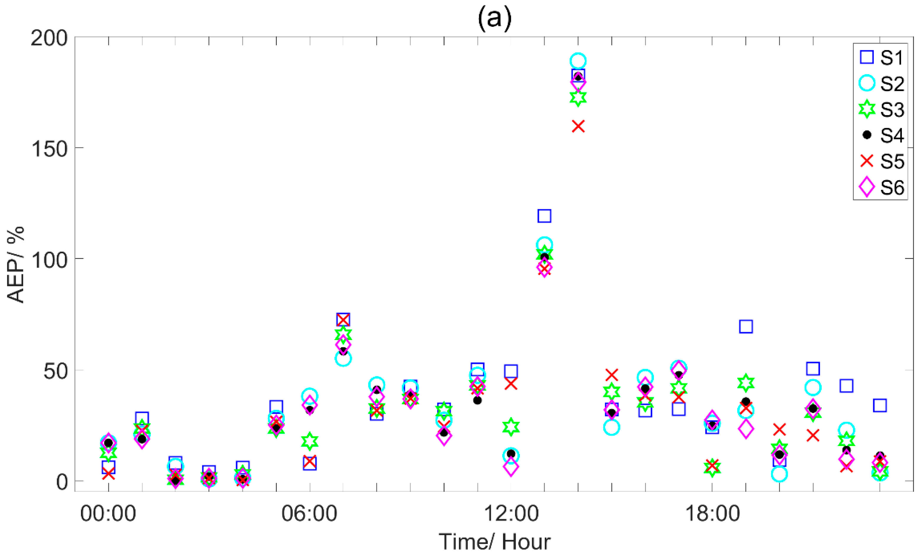
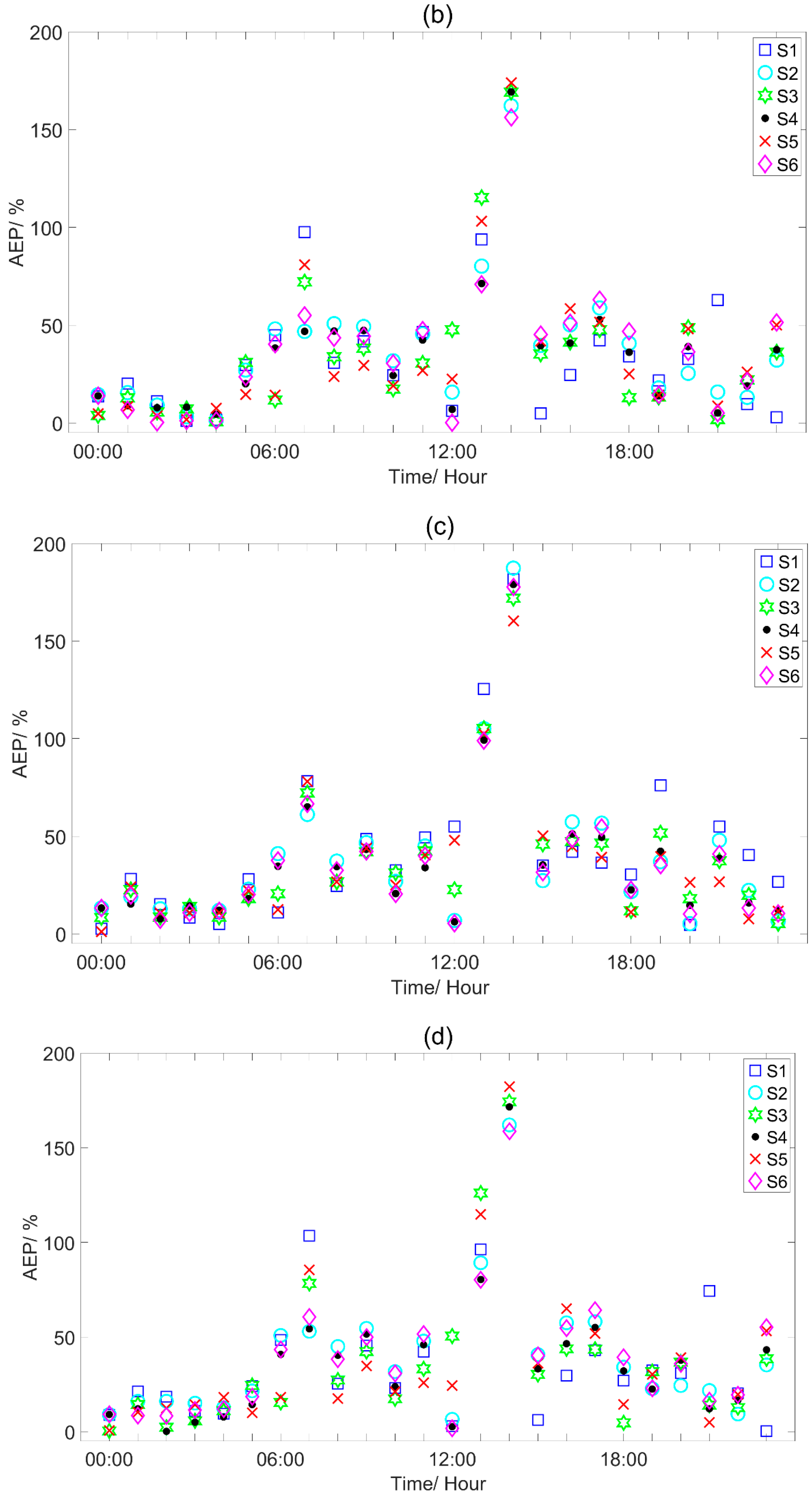
Figure 3 shows the comparison of AEPs for WS simulation at Anxi station with different initial data under different scales of WS. According to the magnitude of WS, the 10-m WS (unit: m∙s⁻¹) at the three stations is divided into ranges by 2 m∙s⁻¹ and 12 m∙s⁻¹, with an interval of 1 m∙s⁻¹ for the evaluation. Results show that the AEP is larger for WS at Anxi station when the WS is below 2 m∙s⁻¹, and it will drop below 100% when the WS is above 2 m∙s⁻¹. The AEP gradually decreases when the WS ranges from 3 to 6 m∙s⁻¹, and there is no significant difference in simulation errors for rest scales. For the simulation with the GFS (Figure 3a), the comparison of parameterization schemes reveals that the AEP of S5 is relatively smaller, basically below 100%, while that S4 is relatively larger. For simulations of ERA5 (Figure 3b), the WS errors are larger than those with the GFS. The AEP is relatively smaller in S1, but larger under S4. Overall, S1 is more suitable for accurate simulations at Anxi station.

From the comparison of simulation results with two initial data, it can be seen that the AEP for the WS with the ERA5 data at Anxi station is relatively larger, mostly above 40%. It should be noted that with the same parameterization schemes, the simulation results differ significantly with different initial data.

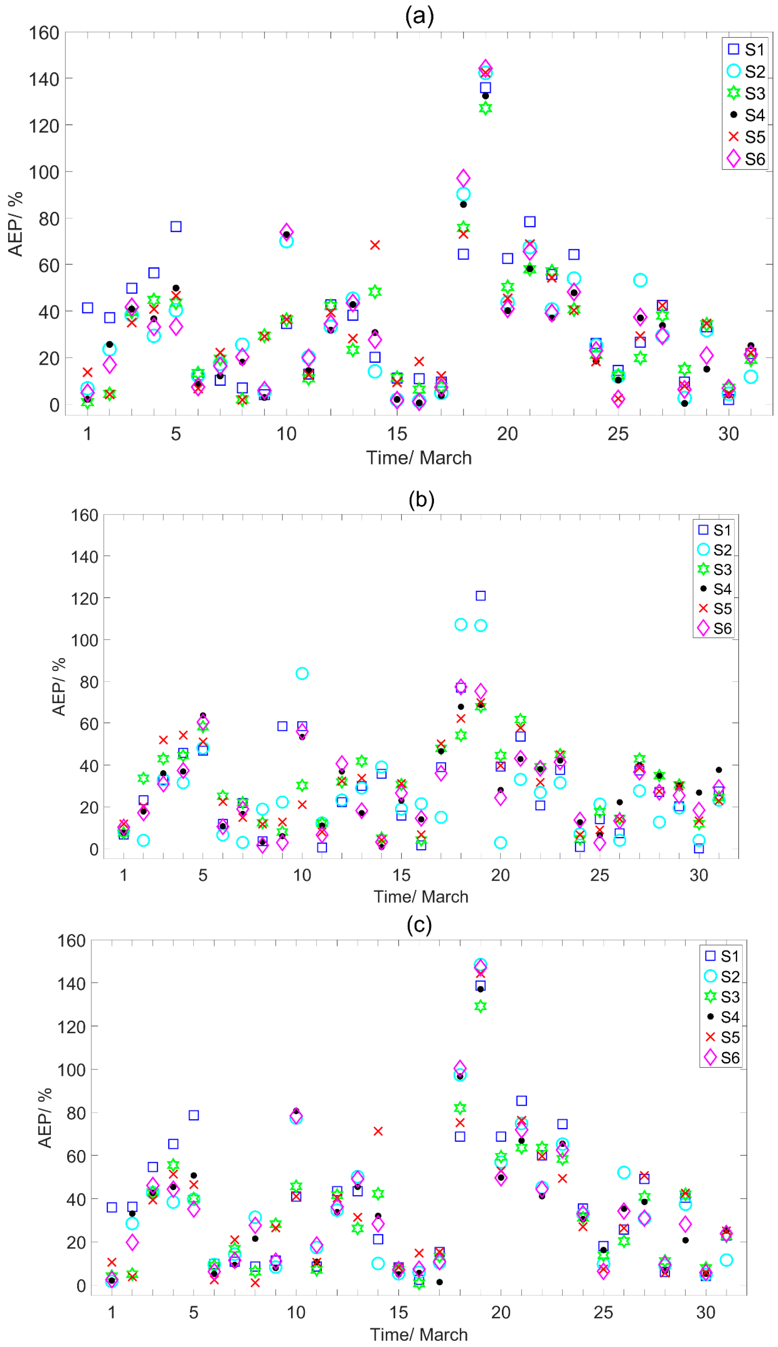
Compared with the results of Anxi station (Figure 3), the difference of simulated WS at Hongliuhe station (Figure 4) among the AEPs under different combinations of parameterization schemes is relatively small, except for WS of less 2 m∙s⁻¹, where the AEPs are above 80%, the AEPs are mostly around 60% at other scales of WS. The AEPs for simulations of S1 and S5 schemes are relatively smaller among all schemes. With the GFS (Figure 4a), the AEP gradually decreases with the WS ranges from 3 to 6 m∙s⁻¹ to 8 to 13 m∙s⁻¹. In contrast, with the ERA5 initial data (Figure 4b), the AEP decreases gradually from 3 to 6 m∙s⁻¹, and subsequently increases with increasing WS. Overall, AEPs of 10-m WS are higher with the ERA5 than the GFS for the simulation.

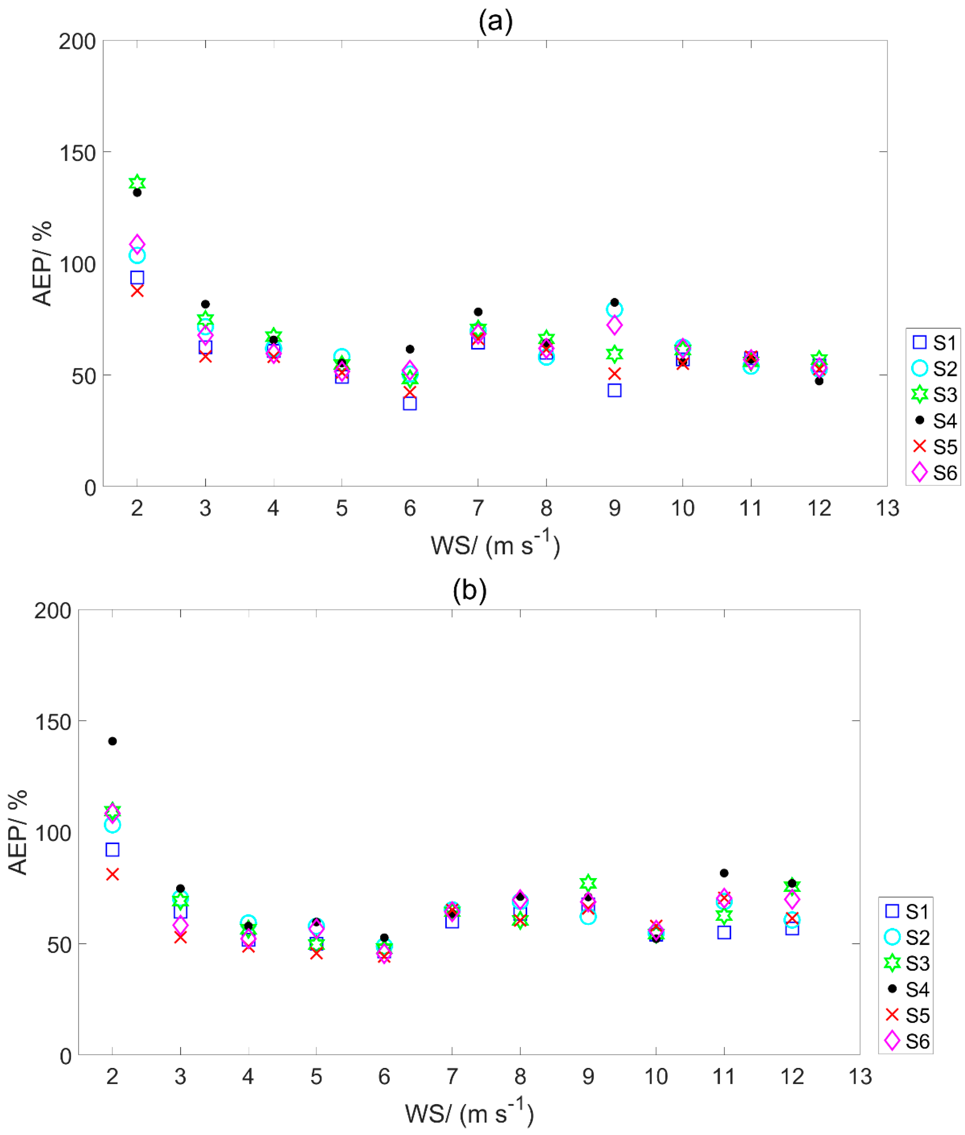
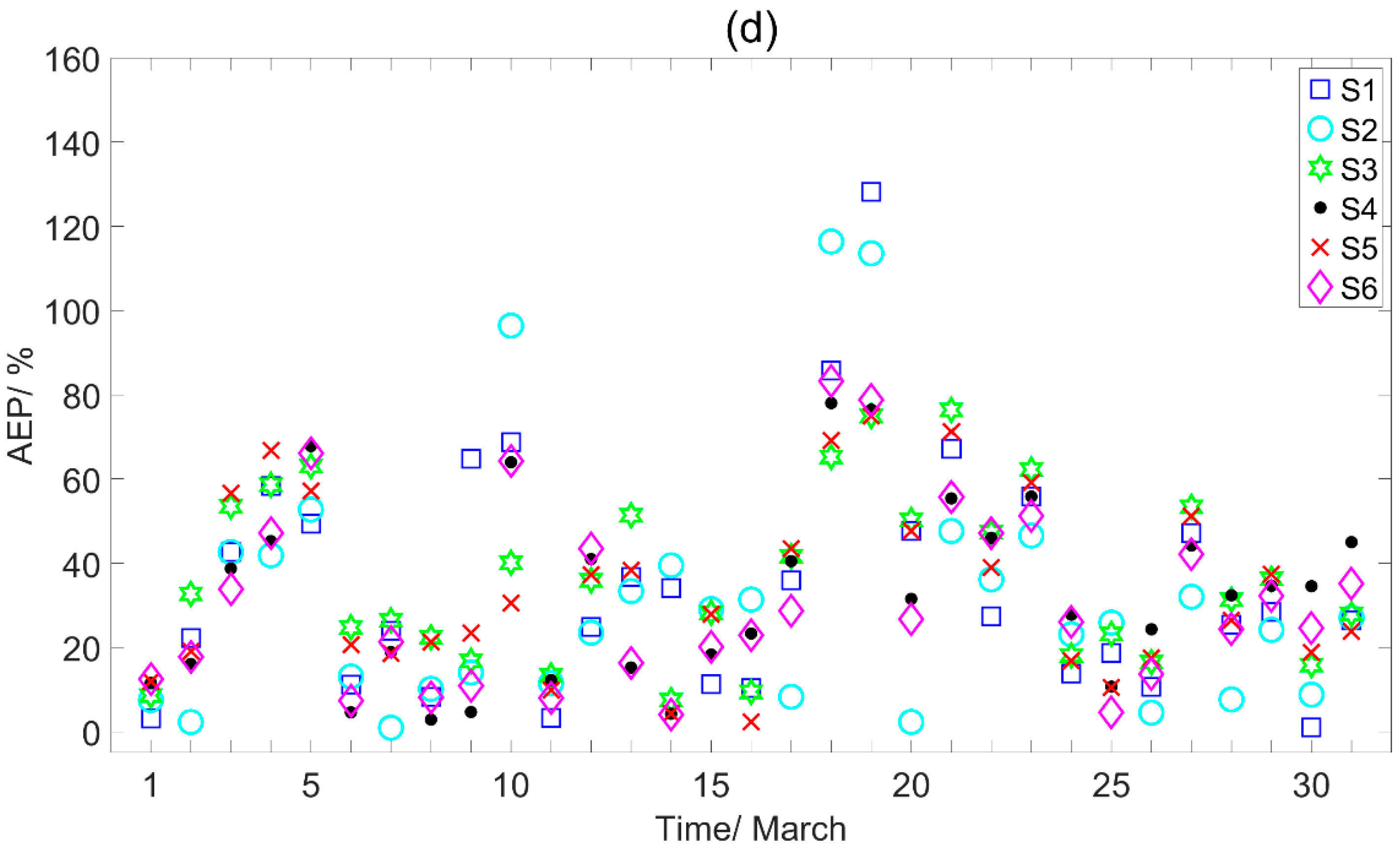
The simulation results at Dunhuang station are shown in Figure 5. When using the GFS driving the model (Figure 5a), the simulation error of WS is relatively large below 2 m∙s⁻¹, which is consistent with the results at Anxi station and Hongliuhe station. As the WS increases, the AEP of the WS simulation also decreases. The AEP is the smallest when the WS is 11 m∙s⁻¹, with a value of below 40%. With the ERA5 (Figure 5b), the simulation has a relatively large AEP and shows a tendency to move from decrease to increase. The AEP is the smallest when the WS is 6 m∙s⁻¹. The comparison between simulation results at three stations shows that S5 has relatively small simulation errors, and thus performs the best.

To further analyze the impacts of different combinations of initial data and parameterization schemes on the WS, the statistical averages of the AEPs at different scales of WS are calculated (

Table 4. AEPs at different stations and averaged AEPs at three stations under different combinations of initial data and parameterization schemes.

AEP/%	Data	S1	S2	S3	S4	S5	S6
Anxi station	GFS	52	73	65	86	51	74
	ERA5	72	91	91	110	75	89
Hongliuhe station	GFS	75	80	89	90	77	77
	ERA5	69	78	81	92	68	79
Dunhuang station	GFS	70	75	76	77	66	69
	ERA5	83	98	91	107	85	97
Average of 3 stations	GFS	66	76	77	84	65	73
	ERA5	75	89	88	103	76	88

). The comparison of AEPs at three stations further reveals that the AEPs are significantly smaller with the GFS (84% and 65% for the maximum and minimum values, respectively) than the ERA5 as the initial field (103% and 75% for the maximum and minimum values, respectively). In comparison with the simulation results of different parameterization schemes, S5 has the smallest value of averaged AEP and thus performs the best. In contrast, with ERA5 data as the initial data, S4 has the largest AEP and performs the worst.

According to the AEPs analyzed in this section and the conclusions about the Rs of WS in Section 4.1, the simulated AEPs of WS at Dunhuang and the surrounding areas are relatively small using the GFS with S5 schemes. Therefore, the YSU + FLG scheme can thus be considered as an optimal combination for 10-m WS simulation. This conclusion can provide a reference for the siting of wind farms in Dunhuang and the surrounding areas, and for the selection of initial data and parameterization schemes in the later forecast of WS.

4.3. Correlation Coefficients for T2

In addition, the simulation accuracy of WS is affected by the simulation result of the T2 [12]. Similarly, the T2 simulation at the above mentioned three stations is obtained under different combinations of initial data, PBL and radiation parameterization schemes. The Rs between and the observed T2 at three stations are shown in Figure 6. Results show that the Rs of the T2 are much higher than that of the 10-m WS (Figure 2). The T2 at Anxi station are all above 0.9, while the effects of different initial data on the simulation results are not significant. The R of the T2 at Hongliuhe station is slightly smaller than that at Anxi station, and the Rs are larger with initial data from the ERA5 than the GFS. There is no significant difference for the Rs of T2 under different combinations of parameterization schemes at Anxi station and Hongliuhe station. The Rs of the T2 at Dunhuang station are significantly smaller than that the other two stations, ranging from 0.8 to 0.9, and the Rs are higher for the ERA5 than the GFS.

To further analyze the effect of different combinations of initial data and parameterization schemes on the T2, statistical results of the average Rs and AEPs for the T2 are shown in

Table 5. Average Rs of T2 for different combinations of initial data and parameterization schemes.

R	S1	S2	S3	S4	S5	S6
GFS	0.89 *	0.91 *	0.91 *	0.92 *	0.89 *	0.91 *
ERA5	0.91 *	0.92 *	0.92 *	0.93 *	0.92 *	0.93 *

Note: * trend significant at a = 0.01.

and

Table 6. Average AEPs at different stations and AEPs averaged at three stations under different combinations of initial data and parameterization schemes.

AEP/%	Data	S1	S2	S3	S4	S5	S6
Anxi station	GFS	1.98	1.81	1.80	1.67	1.99	1.91
	ERA5	1.78	1.76	1.97	2.01	1.56	1.71
Hongliuhe station	GFS	2.96	2.85	2.85	2.77	3.07	2.90
	ERA5	2.79	2.41	2.64	2.31	2.65	2.39
Dunhuang station	GFS	4.90	4.32	4.66	4.26	4.92	4.40
	ERA5	4.65	3.96	4.56	3.91	4.61	3.90
Average of 3 stations	GFS	3.28	2.99	3.11	2.90	3.33	3.07
	ERA5	3.07	2.71	3.06	2.74	2.94	2.67

, respectively. Results show that the Rs are higher by using the ERA5 than the GFS, and the Rs are mostly above 0.9. Compared with the results of simulated WS, the WRF model simulations perform much better on T2 simulation.

4.4. Comparison of Simulated Results with Anemometer Tower Data

4.4.1. Hourly Distribution of Observations from the Anemometer Tower

The hourly distribution of WS at different heights of the anemometer tower in March 2014 is shown in Figure 7. It can be seen that at the 10-m height of the anemometer tower, the WS is mostly below 10 m∙s⁻¹, and the maximum WS appears on 19 March (reaching 19.6 m∙s⁻¹), with an average of 5.7 m∙s⁻¹. Compared with the WS at the height of 10-m WS, the WS at 30 m is relatively larger, which is consistent with previous studies. The average WS at 30 m is 6.2 m∙s⁻¹ with the maximum reaching 21.1 m∙s⁻¹. The WS at 60 m is the largest among the three heights, with an average of 6.6 m∙s⁻¹ and a maximum of 22.4 m∙s⁻¹, and the maximum WS can usually exceed 10 m∙s⁻¹. WS at different heights of the anemometer tower show significant diurnal variations—the WS is relatively smaller during the day and larger at night.

Figure 8 shows the WS and wind direction at different heights of the anemometer tower in March 2014. The WS at 60 m is larger compared with that at heights of 10 m and 30 m, which is consistent with the diurnal variations of WS at different heights. In addition to the WS, the distribution of wind direction is also important to the evaluation of wind energy resources. It can be found that there is no significant difference in the distribution of wind direction at different heights. The dominant wind direction is the northeastern, followed by the southwestern, which is significantly related to the topography distribution. In addition, the distribution for high WS is mainly dominated by the northern wind.

4.4.2. AEPs of Different Initial Data and Parameterization Schemes

Figure 9a presents the daily AEPs for the 30-m WS at the anemometer tower in March 2014 with different combinations of initial data and parameterization schemes. It can be seen that the daily AEP is significantly correlated with the observed WS on that particular day. Larger simulation error of WS corresponds to larger observed WS. On 18 and 19 March 2014, the AEP of simulated WS is also larger due to the larger observed WS, while it is mostly around 40% for the rest of the period. The 30-m WS (Figure 9b) shows a significant decrease in the AEP with the ERA5 than the GFS as the initial data, mostly below 60%, which is significantly different from that of the 10-m WS at regional stations in previous analyses.

The AEP of 60-m WS shows that the difference between different combinations of parameterization schemes narrows as the height in simulated WS rises, and the simulation results are still significantly better for the ERA5 (Figure 10d) than the GFS (Figure 9c). To reveal the differences between different simulations more clearly, the comparison of averaged AEPs are shown in

Table 7. Average AEPs for different combinations of initial data and parameterization schemes.

AEP/%		S1	S2	S3	S4	S5	S6
30 m	GFS	36	32	31	30	33	31
	ERA5	30	27	31	29	29	28
60 m	GFS	38	36	33	34	35	35
	ERA5	35	31	36	33	34	32

.

The WS at different heights of anemometer tower shows that the 30-m WS simulation has a higher AEP by using the GFS than the ERA5 as the initial data (Table 7). With the same schemes, the AEP of the WS simulation with the GFS as the initial data is 6% higher than that ERA5. The conclusions for 60-m WS are consistent with those for 30-m WS, and the AEPs of the simulated WS with the GFS are significantly higher, with a maximum value of 5%. With the WRF model, the simulation error of the 60-m WS is greater than that 30-m WS. WRF model can better simulate the wind speed at the height of 30 to 60 m. This can be intuitively seen from the EP at the heights of 30 and 60 m. The EP of 30–60 m is about 30%. However, the EP at 10-m wind speed is obviously higher. That is because the WRF model presents a high surface wind speed bias over plains or valleys where smoother topography is used and represents a limitation for the high demand for accurate surface wind estimations by different sectors such as wind-energy applications or air-quality studies [21,22].

The AEPs for 30-m and the 60-m WS of the anemometer tower are relatively small compared with the 10-m WS, but no parameterization scheme shows significant advantages at all heights. Overall, it can be concluded that, using the ERA5 as the initial data, and the combination of the ACM2 PBL parameterization scheme and the FLG radiation parameterization scheme, the simulations perform best at all heights.

Wind speed at different heights shows significant diurnal variation. Figure 10 shows the hourly distribution of averaged AEPs of the simulated WS under different combinations of initial data and parameterization schemes in March 2014. Results show that the AEPs of WS vary significantly at different moments, with a significant diurnal variation. The AEP of simulated WS reaches a minimum in the early morning and a maximum in the late afternoon. However, the hourly AEP of the WS with ERA5 is not smaller than that of GFS at every moment. It should be noted that, with the same parameterization schemes, the AEPs of 30-m WS is higher that of 60-m WS. The average AEPs of the hourly WS simulation are complicated, and no parameterization schemes show significant advantages.

5. Summary and Discussion

The main goals of this study were to achieve a better performance of the WRF model in WS near the Dunhuang area and evaluate the impact of initial data, PBL schemes, and radiation schemes on WS simulation. Based on the hourly data of 10-m WS and T2 from the national basic meteorological observing stations in and around Dunhuang (Anxi station, Hongliuhe station, Dunhuang station), as well as the hourly observed WS from the anemometer tower at different heights (10 m, 30 m, 60 m), the WS simulation results near Dunhuang in March 2014 are evaluated. The WS is simulated by the WRF model driven by two datasets (GFS and ERA5), with different combinations of PBL parameterization schemes (ACM2, MYJ, and YSU) and radiation parameterization schemes (RRTMG and FLG). The main conclusions are as follows.

Both GFS and ERA5 data can lead to good results in the spring WRF numerical simulation in northwest China. Among them, GFS is better as a driving dataset in wind speed simulation (maximum correlation coefficients are 0.53 and 0.48 for the GFS and ERA5, respectively), and T2 simulated based on ERA5 is better (maximum correlation coefficients are 0.93 and 0.91 for the GFS and ERA5, respectively).

As the height of the anemometer tower increases, the observed WS increases significantly. The error of the simulated WS is larger when the observed WS is larger. It can be seen from the comparison results of the boundary layer schemes that the YSU scheme has a better simulation effect in northwest China in wind speed and temperature. The YSU scheme considers the impact of clamping effects and enhances the influence of heat in the mixing of the boundary layer, effectively mitigating the problem of excessive mixing of the boundary layer under high wind speed in northwest China. Therefore, its relative error result is the lowest among all tests.

The FLG scheme performs better in wind forecasting, and the RRTMG scheme performs better in temperature forecasting. After comparison and verification, although the radiation parameterization scheme has some differences in the simulation process, it does not produce a decisive advantage. With the ERA5 forcing data, the simulated temperature under the combination of YSU and RRTMG schemes has the highest R and the smallest absolute error.

In this paper, the temperature and WS at observing stations and anemometer towers over the complex underlying surface in the Dunhuang region are simulated and evaluated. The wind simulation performs the best with the GFS as the forcing data, with the YSU and FLG parameterization scheme. Due to the high WS and wind energy density in the local area during the period between winter and spring, this paper focused on the simulation and evaluation in March 2014. However, due to the sparsely observed data from observing stations and anemometer tower, the sample size for comparison is quite limited, thus the reference and representativeness of the findings in this study could be further improved. Therefore, observation data from more anemometer towers should be used in subsequent studies to demonstrate the corresponding spatial applicability. In addition, considering the effect of different seasons on the simulation results, with the increase of the simulation duration, the variability of numerical simulations across seasons could be further obtained. The results of this study would be more robust to evaluate the seasonal sensitivity of initial data and parameterization schemes and minimize the uncertainty of the results.

References

1. Hui, X.Y.; Gao, X.Q.; Gui, J.X.; Liu, J.B.; Deng, G.W. Numerical simulation of high resolution wind power resource in Jiuquan wind power base area. Plateau Meteorol. 2011, 30, 538–544. [Google Scholar]
2. Dowell, J.; Weiss, S.; Hill, D.; Infield, D. Short-term spatio-temporal prediction of wind speed and direction. Wind Energy 2014, 17, 1945–1955. [Google Scholar] [CrossRef]
3. Bilgili, M.; Sahin, B. Comparative analysis of regression and artificial neural network models for wind speed prediction. Meteorol. Atmos. Phys. 2010, 109, 61–72. [Google Scholar] [CrossRef]
4. Zou, J.P.; Zhang, B.D.; Tian, Y. Short term wind speed prediction based on linear combination and error correction. Appl. Mech. Mater. 2014, 521, 135–142. [Google Scholar] [CrossRef]
5. Wang, H.; Yan, J.; Liu, Y.; Han, S.; Li, L.; Zhao, J. Multi-step-ahead method for wind speed prediction correction based on numerical weather prediction and historical measurement data. In Journal of Physics: Conference Series WindEurope Conference & Exhibition 2017, Amsterdam, Netherlands; Volume 926, p. 012007. Available online: https://iopscience.iop.org/article/10.1088/1742-6596/926/1/012007 (accessed on 18 June 2020).
6. Liu, H.; Chen, C.; Tian, H.Q.; Li, Y.F. A hybrid model for wind speed prediction using empirical mode decomposition and artificial neural networks. Renew. Energy 2012, 48, 545–556. [Google Scholar] [CrossRef]
7. Morales, L.; Lang, F.; Mattar, C. Mesoscale wind speed simulation using CALMET model and reanalysis information: An application to wind potential. Renew. Energy 2012, 48, 57–71. [Google Scholar] [CrossRef]
8. Yuan, Y.; Xiaoli, L.I.; Chen, J.; Xia, Y. Stochastic parameterization toward model uncertainty for the GRAPES mesoscale ensemble prediction system. Meteorol. Mon. 2016, 1161–1175. [Google Scholar]
9. Li, D.; Zhou, X.; Chen, L.; Yang, S.; Wang, S. Wind speed forecasting method based on numerical model. Acta Energ. Sol. Sin. 2012, 33, 1683–1689. [Google Scholar]
10. Che, Y.; Peng, X.; Delle Monache, L.; Kawaguchi, T.; Xiao, F. A wind power forecasting system based on the weather research and forecasting model and Kalman filtering over a wind-farm in Japan. J. Renew. Sustain. Energy 2016, 8, 013302. [Google Scholar] [CrossRef]
11. Cristian, M.; Borvarán, D. Offshore wind power simulation by using WRF in the central coast of Chile. Renew. Energy 2016, 94, 22–31. [Google Scholar]
12. Mirocha, J.D.; Simpson, M.D.; Fast, J.D.; Berg, L.K.; Baskett, R.L. Investigation of boundary-layer wind predictions during nocturnal low-level jet events using the Weather Research and Forecasting model. Wind Energy 2016, 19, 739–762. [Google Scholar] [CrossRef]
13. Zhang, T.; Li, Y.; Duan, H.; Liu, Y.; Zeng, D.; Zhao, C.; Gong, C.; Zhou, G.; Song, L.; Yan, P. Development and evaluation of a WRF-based mesoscale numerical weather prediction system in northwestern China. Atmosphere 2019, 10, 344. [Google Scholar] [CrossRef] [Green Version]
14. Shen, X.Y.; Yan, Y.Q.; Xiao, H.B.; Quan, C. Influence on simulation of temperature, precipitation and wind speed by using fifferent combinations of parameterization schemes in WRF model in Qinghai province. J. Arid Meteorol. 2018, 36, 423. [Google Scholar]
15. Yuanyuan, M.A.; Yang, Y.; Xiaoming, H.U.; Youcun, Q.I.; Zhang, M. Evaluation of three planetary boundary layer parameterization schemes in WRF model for the February 28th, 2007 gust episode in Xinjiang. Desert Oasis Meteorol. 2014, 8, 8–18. [Google Scholar]
16. Tao, S.U.; Miao, J.F.; Wang, Y.H. Impact of radiative transfer parameterizations on simulated sea breeze thunderstorm over the Hainan Island. Chin. J. Geophys. 2017, 60, 3023–3040. [Google Scholar]
17. Carvalho, D.; Rocha, A.; Gómez-Gesteira, M.; Santos, C. A sensitivity study of the WRF model in wind simulation for an area of high wind energy. Environ. Model. Softw. 2012, 33, 23–34. [Google Scholar] [CrossRef] [Green Version]
18. Zou, Z.C.; Deng, Y.C. Comparison of wind speed prediction in WRF model based on NCEP GFS and JMA GSM forecasting fields. Water Resour. Power 2016, 34, 194–197. [Google Scholar]
19. Wang, Y.; Yang, Y.; Zhang, F.M.; Yang, L.L. Improve the forecast of surface-layer wind in wind power farm with WRF-3DVAR. Adv. Mater. Res. 2013, 724, 480–484. [Google Scholar] [CrossRef]
20. Cheng, X.H.; Tao, S.W.; Wei, L.; Wei, D.; Chen, J.M.; Jiang, Y. Short-term wind power forecasting experiment based on WRF model and adapting partial least square regression method. Plateau Meteorol. 2012, 31, 1461–1469. [Google Scholar]
21. Jiménez, P.A.; Dudhia, J. Improving the representation of resolved and unresolved topographic effects on surface wind in the WRF Model. J. Appl. Meteorol. Climatol. 2012, 51, 300–316. [Google Scholar] [CrossRef] [Green Version]
22. Mass, C.; Ovens, D. Fixing WRF’s high speed wind bias: A new subgrid scale drag parameterization and the role of detailed verification. In Proceedings of the 24th Conference on Weather and Forecasting/20th Conference on Numerical Weather Prediction, Seattle, WA, USA, 22–27 January 2011. [Google Scholar]
Figure 1. Simulation domains used in the model (a) and terrain height (b) (shading; Unit: m) of Domain 3 (D03). A: Hongliuhe Station; B: Anxi Station; C: Dunhuang Station; D: Anemometer tower.
Atmosphere 11 00647 g001
Figure 2. Correlation coefficients between 10-m simulated wind speed (WS) and observed WS with the combinations of different initial data and different parameterization schemes.
Atmosphere 11 00647 g002
Figure 3. Absolute error percentage (AEP) distributions of WS simulation at Anxi station for different scales of WS. Simulation result with (a) the global forecast system (GFS), and (b) the ERA5.
Atmosphere 11 00647 g003
Figure 4. Same as Figure 3, but for Hongliuhe station.Simulation result with (a) the global forecast system (GFS), and (b) the ERA5.
Atmosphere 11 00647 g004
Figure 5. Same as Figure 3, but for Dunhuang station.Simulation result with (a) the global forecast system (GFS), and (b) the ERA5.
Atmosphere 11 00647 g005
Figure 6. Correlation coefficients between simulated 2-m temperature (T2) and observed T2 with the combinations of different initial data and different parameterization schemes.
Atmosphere 11 00647 g006
Figure 7. Diurnal variations of WS at heights of (a) 10 m, (b) 30 m and (c) 60 m of the anemometer tower in March 2014 (unit: m∙s−1).
Atmosphere 11 00647 g007aAtmosphere 11 00647 g007b
Figure 8. Distributions of wind roses at heights of (a) 10 m, (b) 30 m, (c) 60 m of the anemometer tower in March 2014.
Atmosphere 11 00647 g008
Figure 9. Distributions of daily AEPs for different parameterization schemes. (a,b) are the results of 30 m, (c,d) are the results of 60 m. (a,c) are the simulation results with the GFS as the initial data; (b,d) are the simulation results with the ERA5 as the initial data.
Atmosphere 11 00647 g009aAtmosphere 11 00647 g009b
Figure 10. Same as Figure 9, but for distributions of hourly AEPs.(a,b) are the results of 30 m, (c,d) are the results of 60 m. (a,c) are the simulation results with the GFS as the initial data; (b,d) are the simulation results with the ERA5 as the initial data.
Atmosphere 11 00647 g010aAtmosphere 11 00647 g010b