Review

Atmospheric Pollutant Dispersion over Complex Terrain: Challenges and Needs for Improving Air Quality Measurements and Modeling

1
Department of Civil, Environmental and Mechanical Engineering, University of Trento, 38123 Trento, Italy
2
Department of Science and Technological Innovation, University of Eastern Piedmont, 15151 Alessandria, Italy
3
Department of Atmospheric and Cryospheric Sciences, University of Innsbruck, 6020 Innsbruck, Austria
4
Université Grenoble Alpes, CNRS, Grenoble INP, LEGI, 38000 Grenoble, France
5
Institute of Atmospheric Sciences and Climate, National Research Council, 10133 Torino, Italy
6
C3A—Center Agriculture Food Environment, University of Trento, 38010 San Michele all’Adige, Italy
*
Author to whom correspondence should be addressed.
Atmosphere 2020, 11(6), 646; https://doi.org/10.3390/atmos11060646
Submission received: 27 May 2020 / Revised: 13 June 2020 / Accepted: 16 June 2020 / Published: 18 June 2020
(This article belongs to the Special Issue Atmospheric Processes over Complex Terrain)

Abstract

:
Pollutant dispersion processes over complex terrain are much more complicated than over flat areas, as they are affected by atmospheric interactions with the orography at different spatial scales. This paper reviews recent findings and progress in this field, focusing on both experimental and modeling perspectives. It highlights open questions and challenges to our capability for better understanding and representing atmospheric processes controlling the fate of pollutants over mountainous areas. In particular, attention is focused on new measurement techniques for the retrieval of spatially distributed turbulence information and air quality parameters, and on challenges for meteorological and dispersion models to reproduce fine-scale processes influenced by the orography. Finally, specific needs in this field are discussed, along with possible directions for future research efforts.

1. Introduction

Many mountains in the world are undergoing a process of increasing anthropization. Indeed, nowadays roughly 900 million people, i.e., 13% of the world’s population, live in mountainous regions [1,2]. An even higher number of persons are attracted to mountainous areas for tourism and recreational activities every year. For example, in the Alps, an overall demand of more than 464 million overnight stays per year is estimated [3]. Moreover, populations living in mountain regions increasingly concentrate in rapidly expanding urban areas; it is estimated that roughly 30% of the world’s mountain population lives nowadays in cities, and this percentage reaches 50% in developed countries [2].
Mountain valleys and passes are also often crossed by main transport routes connecting different countries. For example, the Alps are crossed by 4200 km of main roads, with 6 million vehicles and 1.24 × 10¹¹ kg of freights being transported across the Alpine range every year [4]. As a consequence, the anthropogenic impact on mountainous areas raises concerns from many viewpoints. In particular, one of the most serious hazards involves pollutant emissions and their effects on air quality. Major sources of pollutants in mountainous regions are generally located inside valleys and basins, where the main urban areas and traffic routes develop, and most of the population lives. This is shown, as an example, in Figure 1, displaying annual emissions of NOx and PM10 in South Tyrol, in the Italian Alps [5]. Under unfavorable meteorological situations, pollutants may accumulate at the bottom of valleys and basins, implying that a large part of the population is potentially exposed to high concentrations. In fact, in such conditions, atmospheric dispersion, i.e., the combined effect of transport/advection by the mean wind and diffusion due to turbulent mixing, may be strongly inhibited. High levels of pollutants are harmful, not only to humans, wildlife and livestock, but may also cause damage to the environment, especially vegetation and forest heritage [6]. Furthermore, pollutants may be transported by orographic flows towards mountainous areas from adjacent regions, where they are emitted. As a consequence, significant concentrations of harmful species, especially secondary pollutants, may also be found in areas where they were not locally emitted [7,8,9].
The relevance of the problem of pollutant dispersion has been a primary driver for many research efforts focused on atmospheric processes over complex terrain in recent decades. In fact, the need for better understanding and suitable modeling of the fate of pollutants in mountainous regions stimulated a number of projects, which involved both experimental activities, such as extensive field campaigns in complex environments, and the advancement of new modeling capabilities over complex terrain, encompassing both meteorological and air quality models. Among the projects primarily focusing on the study of air pollution dispersion over complex terrain, it is worth mentioning Monitoring and minimization of traffic-induced noise and air pollution along major Alpine transport routes (ALPNAP) [10,11,12], Bolzano Tracer Experiment (BTEX) [13,14], Persistent Cold-Air Pool (PCAPS) [15], Transport of Air Pollutants over Complex Terrain (TRACT) [16], Mesoscale transport of atmospheric pollutants across the central Alps (TRANSALP) [17,18], Vertical Ozone Transports in the Alps (VOTALP) [19], and Vertical Transport and Mixing (VTMX) [20]. Other projects aiming at characterizing dispersion in complex terrain and directly or indirectly focusing on air pollution will be reviewed in this paper. Results from these projects have greatly contributed to the advancement of knowledge in this field. However, several aspects, concerning both our understanding and our ability of observing and modeling processes related to pollutant dispersion over complex terrain, still remain to be investigated. In fact, the understanding and the quantification of pollutant dispersion over complex terrain are much more difficult than over flat areas, as dispersion processes are affected by atmospheric interactions with the orography at different spatial scales. In particular, atmospheric flows over complex terrain are characterized by a continuous and interacting range of scales, from synoptic forcing to mesoscale circulations and turbulence fluctuations. In complex terrain, the mechanical and thermal influence of the orography can modify the large-scale flow and produce smaller-scale motions which would not exist on flat terrain [21,22,23], thus enhancing the spatial and temporal variability of atmospheric processes relevant for pollutant dispersion.
Based on these considerations, this paper aims at reviewing recent research activities focusing on several aspects connected to pollutant dispersion over complex terrain, from both experimental and numerical modeling perspectives. A review of recent progress in the field will lead to open questions and challenges for improving our capability to better understand and represent atmospheric processes responsible for the fate of pollutants over complex terrain. Following this objective, the present paper is organized as follows. Section 2 contains a general overview of the processes affecting pollutant transport and diffusion over complex terrain, focusing in particular on the peculiarities of atmospheric processes over mountains when compared to flat terrain. Section 3 is dedicated to measurement techniques supporting air quality management and the understanding and modeling of atmospheric dispersion processes, with a focus on new observational techniques, remote sensing, and innovative low-cost sensors for air quality monitoring. Section 4 and Section 5 concentrate on numerical modeling and provide an overview of the state of the art and perspectives of both meteorological and dispersion modeling. Finally, conclusions and an outlook for future research needs are given in Section 6.

2. Atmospheric Processes and Pollutant Dispersion over Complex Terrain

The concentration of pollutants in the atmospheric boundary layer (ABL) depends not only on emissions, but also, and sometimes crucially, on atmospheric dispersion. High concentrations of pollutants therefore follow not only from strong emissions, but also from reduced dispersion, especially in the atmospheric layer adjacent to the surface, where most of the pollutants are emitted.

2.1. Temperature Stratification

Temperature stratification (static stability) is one of the main factors controlling turbulent mixing in the atmosphere: the most critical situations occur under wintertime anticyclonic episodes, when radiative cooling at the ground leads to the formation of a very stable air layer above the surface. This situation is usually referred to as ground-based inversion; it inhibits turbulent motions, and consequently keeps pollutants “trapped” in that layer [24,25,26,27,28,29]. This situation may last for several days to several weeks, and is more frequent in mountainous regions; here the reduced sky-view factor limits the penetration of solar radiation into valleys and basins, and the nocturnal drainage winds favor the accumulation of cold air at low levels.

2.2. Mountain Boundary Layer Height

A key parameter affecting pollutant concentration is the height of the ABL, as it determines the volume of atmosphere available for pollutant dispersion. Turbulent mixing comes again into play, since it also contributes to controlling the evolution of the ABL depth. Over flat terrain, the depth of the ABL can often be assumed to be horizontally homogeneous, whereas over complex terrain the so-called “mountain boundary layer” (MoBL) [30] is spatially highly inhomogeneous and interacts with mesoscale flows. As a consequence, an accurate determination of the height of the MoBL is a more difficult task than over flat areas [30]. In fact, apart from quite substantial uncertainty arising from data quality and parameter choices even over flat terrain (cf., e.g., [31]), at least well-established criteria are available in the literature. Conversely, more interacting factors contribute to the spatio-temporal variability of the MoBL height in complex terrain, as extensively discussed in a recent review paper [32]. For example, heterogeneity in the penetration of solar radiation in mountain valleys and basins can produce significant spatial variability in the surface energy budget, influencing both atmospheric stratification and the boundary layer height [33,34]. Additionally, quantities defining the reference “boundary layer height” based on classical (i.e., flat terrain) concepts under convective conditions, do not, in general, correspond to the height up to which mixing is effective (i.e., the MoBL height). For example, Lang et al. [35] highlighted, using idealized large eddy simulations (LES), that different definitions of the boundary layer height yield similar results over flat terrain (Figure 2a), while significant discrepancies arise when idealized topographic features are introduced into the simulation (Figure 2b). Likewise, under stable stratification, the height of the boundary (inversion) layer can be modulated by the interaction of the upper-level wind with down-valley flows of tributary valleys, as the direction of the upper-level wind varies during the stable episode [36].

2.3. Strong Synoptic Forcing

When the upper-level wind speed is considered, two main situations affecting pollutant dispersion in the lowest layers in mountainous regions can be distinguished. One situation occurs with strong upper-level wind speed, associated with a significant synoptic forcing. Over a plain, these conditions usually favor the dispersion of pollutants. However, in mountainous terrain, depending on the alignment of the upper-level wind with the valley axis [38], the valley bottom may be sheltered from downward intrusions of the wind from above. Additionally, the penetration of the upper-level wind down to the lowest levels of valleys and basins may be further prevented by underlying pre-existing and persistent stable layers, such as those associated with nighttime cooling, especially in wintertime [39]. Under these conditions, the flow inside valleys is decoupled from the airflow situation above the crest level, and the persistence of such conditions (i.e., light local flows and stable stratification) favors pollutant accumulation at the lowest levels.

2.4. Weak Synoptic Forcing and Thermally Driven Flows

The second situation occurs under persistent anticyclonic pressure fields, generally associated with weak synoptic forcing and clear skies. In this case, the circulation inside the valley or basin is driven by the local heating and cooling of the air layers adjacent to the ground, leading to down-slope and down-valley flows during the night and up-slope and up-valley flows during the day [40,41]. The slope and valley flows control the transport and the diffusion of pollutants. In summer, the up-slope and up-valley flows are generally well developed, and may be associated with convective cells, which can extend very high above the valley bottom, up to a few kilometers, thus transporting pollutants to high altitudes [42]. In this case, up-slope circulations strongly enhance the mass exchange between the valley boundary layer and the free atmosphere with respect to pure turbulent exchange [43]. On the contrary, in wintertime, due to the reduced heating of the valley atmosphere, down-slope and down-valley flows dominate the valley circulation [44,45]; as shown in [46] from numerical simulations in the Grenoble Valley, this “nighttime” flow regime may last about 18 h (over 24 h), ceasing only for a few hours around midday, during which a weak convective activity may be observed above the valley bottom over a height of, at most, 50 m. In these situations, wind speed is generally weak (less than 1.5–2 m s−1), with frequent calm regimes (with wind speed less than 0.5 ms−1) and an inversion layer characterized by a positive temperature gradient can form in the valley up to an altitude close to the crest level. As a result, pollutant dispersion is strongly reduced during a wintertime episode [47,48]. In low wind speed conditions, pollutant dispersion is governed by meandering, a phenomenon still largely under study (see a brief review in [49]), dispersing plumes over wide angular sectors [23].
The inversion layer, typical of these wintertime episodes, along with topographic effects, leads to the formation of stagnation and ventilation zones [50,51]. In the sections of the valley displaying a nearly basin-like structure, stagnation zones develop in which pollutants travel over short distances from their emission points [11,52]. In these stagnation zones, pollutant concentrations increase steadily in time during the episode [53,54]. On the other hand, in ventilation zones, such as a valley section opening onto a plain, ventilation effects lead to the evacuation of pollutants [29]. The end of the persistent anticyclonic wintertime episode occurs when the upper-level wind is able to reach the valley floor and/or the energy input is sufficient to break up the inversion layer [55]. As a result, pollutants can be transported above crest level by vertical fluxes or out of the valley by the channeled wind. An example of the progressive accumulation of pollutants on the valley floor during an anticyclonic wintertime episode is reported in Figure 3. This figure displays a time–height plot of wind speed measured by a SODAR (SOnic Detection And Ranging), along with PM10 concentration, during a field campaign of the ALPNAP project in the Alpine Adige Valley [11]. It can be noted that PM10 concentration remains low in the first three days, when moderate winds reach the valley floor. On the other hand, a progressive accumulation of PM10 occurs in the subsequent days, characterized by weak winds, until a progressive increase in the wind speed terminates the air pollution episode.
Thermally driven circulations affect the transport of pollutants in many other different ways. For example, valley winds may advect highly polluted air downstream from major pollutant sources. Conversely, valley circulations may also have a cleansing effect, when cleaner air is transported into polluted regions. More generally, pollutant transport by a down-valley flow depends both upon the stratification in the valley and upon local orographic features. Indeed, if a strong ground-based inversion exists at the valley bottom, the down-valley wind may detrain at its level of neutral buoyancy, leaving the valley bottom unperturbed. The detrainment may be also associated with the excitation of internal gravity waves [36,56,57], which may result in fluctuations of the pollutant concentration [29]. On the other hand, up-slope or up-valley winds may advect primary pollutants or precursors (also from natural sources, such as forests) to upper levels in the atmosphere; there, the different exposure to stronger radiation and/or other ambient conditions may affect (photo)chemical reactions, producing secondary pollutants (e.g., ozone), which eventually get drained to lower levels by nocturnal down-slope flows. At larger spatial scales, plain-to-mountain circulations can advect pollutants and their precursors towards mountain ranges [58], where they may be embedded into smaller scale circulations, and eventually transported into the free atmosphere (a process referred to as “mountain venting” [59,60,61]), also depending upon the geometry of the mountain range.
The development of thermally driven circulations is strongly affected by land cover heterogeneities, which are more common in mountainous areas. Changes in surface properties (such as albedo, thermal capacity, and conductivity) between valley floors, sidewalls, and mountain tops may modify surface–atmosphere heat exchanges and thermal contrasts driving these local circulations. Other climatic influences being equal, mountainous areas are more likely to have snow-covered terrain for a significant part of the year. Snow cover has many effects on the surface layer. First, snow cover on the ground affects the thermal structure, favoring stable stratification. Moreover, irregular snow cover, typically associated with the different exposure to the solar radiation of the valley sidewalls or with the varying altitude of the valley floor, may also produce asymmetric local circulations, influencing the redistribution of pollutants [52]. The higher amount of reflected radiation from extended snow-covered areas may also favor photochemical reactions, leading to an increased production of secondary pollutants [62,63].

2.5. Urban Areas

Local circulations may also be affected by land cover heterogeneity associated with extended urban areas. Indeed, cities usually experience higher near-surface temperatures, especially during nighttime [64], leading to the so-called “urban heat island” effect. Higher urban temperatures can cause the development of an “urban breeze”, with convergent motions toward the city center at low levels [65]. Thermal hot-spots induced by urban areas may superimpose to the temperature gradients developing inside valleys, and locally modify the normal along-valley horizontal pressure gradients driving the diurnal pattern of up- and down-valley flows [66]. This usually implies a wind convergence over the city, especially during nighttime, when the urban heat island is stronger, thus favoring the accumulation of air pollutants [67]. Moreover, the higher roughness associated with buildings may produce an internal urban boundary layer [68], preventing or limiting the penetration of flows and the ventilation into the urban canopy [69,70]. Similar to the action of upper-level winds on the circulation in a valley, the orientation of urban canyons with respect to the flow direction may determine very different internal circulations, resulting in better ventilation in streets aligned with the mean flow. As a consequence, in cities lying within valleys, streets aligned along the main valley axis are usually better ventilated. Urban areas can also modify the development of the ground-based temperature inversion at night [71,72], as well as its break-up in the morning, with a significant impact both on air quality and on the cross-valley wind system [73,74]. All these aspects still make the case of urban areas over complex terrain a particularly challenging situation.

3. Observational Techniques Supporting Air Quality Management and Pollutant Dispersion Modeling

3.1. Meteorological Measurements

For the assessment (i.e., interpretation, understanding, and modeling) of pollutant dispersion processes anywhere in the world, mean flow characteristics (such as wind speed and direction, stratification, etc.) are required for characterizing advection, as well as information on the turbulence state, which is needed to evaluate diffusion processes. Measurements to assess mean meteorological variables are usually available from meso-networks—albeit generally not at the spatial resolution one would wish. This is particularly true over mountains, where the maintenance and operation of meteorological networks can be highly demanding [75]. On the other hand, measurements of turbulence variables to assess air quality in mountainous terrain are largely unavailable from routine networks. Datasets for these variables therefore stem from research projects with limited duration. One of the first projects was Atmospheric Studies over Complex Terrain (ASCOT) [76], in 1984—even if this study only had a (small) number of “representative” turbulence sites. More recent projects that focused on turbulence and exchange processes in complex terrain—or at least had a strong component on this topic—include ALPNAP in 2005–2008 in the Alps [10,11,12], Boundary Layer Late Afternoon and Sunset Turbulence (BLLAST) in 2011 in southern France [77], Convective and Orographically induced Precipitation Study (COPS) in 2007 in southern Germany [78], Mesoscale Alpine Programme–Riviera (MAP) in 1999 in the Riviera Valley [79], Mountain Terrain Atmospheric Modeling and Observations (MATERHORN) in 2012–2015 in Utah [80], Meteor Crater Experiments (METCRAX and METCRAX II) in 2006–2009 and 2013–2016 in Arizona [81,82], Persistent Cold-Air Pool (PCAPS) in 2010–2011 in Salt Lake Valley [15], Terrain-Induced Rotor Experiment (T-REX) in 2003–2006 in Owens Valley [83], and Vertical Transport and Mixing (VTMX) in 2000 in Salt Lake Valley [20]. All these projects resulted from collaborative efforts and hence were able to measure multiple sites in order to address the problem of spatial variability, which is inherent to boundary layer processes in non-flat terrain [84].
As for long-term measurement installations for turbulence-related variables, there are a handful of “fluxnet towers” (as part of global CO2 monitoring activities) [85] situated in mountainous terrain (e.g., in Switzerland: Davos [86], in Italy: Ritten/Renon [87], Lavarone [88], and Mt. Bondone [89], and in Austria: Neustift [90]). With the “i-Box” in the Austrian Inn Valley [91] there is, furthermore, a long-term program running, which currently aims at, among others things, providing turbulence data from six sites, which have been selected for their representativeness of particular types of surfaces (valley floor, slope (exposition and slope angle), mountain top, etc.).
Turbulence measurements over complex, mountainous terrain are generally performed with the same instrumentation as over flat terrain, i.e., sonic anemometers/thermometers (point observations), scintillometers (spatially averaged fluxes), and more recently, wind profilers (lidars, sodars) and airborne observations. Due to the terrain complexity, they all exhibit their specific challenges, which are briefly summarized in the following section.

3.1.1. Point Measurements

The post-processing of sonic data includes quality control, coordinate rotation, and the correction of known physical effects (e.g., Webb-Pearman-Leuning (WPL) correction), as summarized and discussed in [22,92,93]. In particular, Falocchi et al. [22] and de Franceschi et al. [93] suggested methods to separate low-frequency components, associated with mean flow and larger vortexes, from smaller scale turbulence responsible for turbulent diffusion. Additionally, over sloping terrain, the coordinate rotation requires particular attention. Both the double rotation (DR) and planar fit (PF) approaches rely on a coordinate system that is normal to the surface [94]. Given the instrument layout of most sonic anemometers (having the least systematic errors for flow parallel to the instrument), these instruments should be installed with the best viewing side normal to the local surface. No clear preference could be found so far concerning DR vs. PF, except that PF seems to have advantages for climatological applications (e.g., long-term CO2 flux assessment) while DR better corresponds to the assessment of, e.g., local similarity relations. In addition, PF may require more than sectorial planes [92]. For the purpose of comparing measurements to model output, it is relevant that they both refer to the same coordinate framework (vertical vs. normal to the slope), since along-slope turbulent heat fluxes can contribute to the vertical (as opposed to normal) turbulent heat flux considerably, thus influencing stability [95,96].
Many of the “best practice procedures” for the analysis of turbulence measurements in complex terrain are relatively recent and based on the respective authors’ datasets (site characteristics, season, duration, etc.). Therefore, it would be highly desirable to work out an overall best practice, based on systematically comparing different approaches, and their combinations, using different datasets.

3.1.2. Scintillometry

The retrieval algorithm of scintillometry depends on the applicability of scaling relations. Generally, commercial instruments use similarity relations for the temperature structure function based on Monin–Obukhov similarity theory (MOST) (which is strictly valid for the horizontally homogeneous, stationary surface layer only) to derive spatially averaged turbulent fluxes. Thus, the application of scintillometry strongly depends on the applicability of generic MOST relations in complex terrain. Weiss [97] and Weiss et al. [98] found relatively favorable correspondence between scintillometry-derived and point measurements (heat flux) over a gentle local slope. Pianezze [99] reported substantial deviations from “ideal behavior” for the structure functions depending on cross-sections over a steep Alpine valley (the Mesolcina Valley in southern Switzerland). Ward [100] listed a (small) number of additional applications of scintillometry over gentle topography. From Ward’s considerations, it can be concluded that it is particularly important to use an accurate effective beam height, which may be difficult to determine over complex terrain. Hartogensis et al. [101] discussed how to calculate the effective beam height, taking into account varying beam height along the path and its impact on the measured structure parameter (they do not, however, really address any complex orography in this paper).
For a successful application of scintillometry in mountainous terrain, therefore, it is necessary to assess in more detail the applicability (conditions, situations) of MOST relations for the structure parameters, as well as to possibly derive more appropriate parameterizations. Given the potential of scintillometry for model validation (the comparison of inherently spatially averaged turbulent fluxes from model grids with spatially averaged observations), the further development of this area of research is highly desirable.

3.1.3. Lidars

Wind and temperature/humidity lidars are powerful tools to assess the temporal/spatial structure of meteorological variables near the surface, e.g., [102], which is especially useful in complex terrain with its inherently inhomogeneous flows, e.g., [103]. Furthermore, lidar technology allows, in principle (and under suitable conditions, e.g., stationarity during the averaging interval), the retrieval of turbulent (integral) statistics, such as the vertical velocity variance. Depending on the number of instruments involved and the scan strategy, profiles or point information at a specified location in the atmosphere can be retrieved [104]. Retrieval algorithms and the corresponding accuracy [105] of the obtained turbulence information is an area of active research even over flat terrain and has received an increased interest since the availability of commercial wind lidars.
There are only very few applications to date using lidars to retrieve turbulence statistics in complex terrain, e.g., [106,107,108,109]. For example, Adler and Kalthoff [110] have used profiles of vertical velocity moments (variance and skewness) to determine the local MoBL height. Still, the application of lidars to obtain turbulence information in complex terrain is at its infancy and—based on the importance of such information for the simulation or understanding of pollutant dispersion processes in complex terrain—requires a major boost in the near future.

3.1.4. Airborne Observations

Airborne measurements constitute another well-suited platform to detect, not only the mean thermal and dynamical structure, but also turbulence properties controlling the diffusion of pollutants over complex terrain. As to the mean variables, de Franceschi et al. [111] and Laiti et al. [112,113,114] have successfully retrieved the vertical thermal structure associated with valley winds in Alpine valleys by means of measurement flights along carefully designed trajectories, and subsequent data analysis including spatialization via geostatistical techniques (kriging). As to turbulence properties, in principle, traditional methods (Fourier transform of time series, Reynolds decomposition) can be used—with a number of caveats concerning stationarity and homogeneity—to retrieve turbulent statistics. In relation to topographic flows, flights are often conducted relatively far above the terrain, e.g., [115,116] for obvious safety reasons. Weigel et al. [117] have used data from a light research aircraft within and above a relatively small valley to investigate the turbulent kinetic energy (TKE) structure using the Reynolds decomposition technique along flight paths and found favorable agreement with surface-based tower data for “fly-bys”. The wavelet transform has been used to obtain information on the spatial variability of, e.g., turbulent fluxes from airborne data, e.g., [118]. Even if some caveats exist here as well [116], Baur [119] has successfully used this approach to investigate the spatial structure of turbulence characteristics in the Inn Valley located in Austria. This processing does not come without possible limitations. In particular, the finer resolution comes at the expense of (large) uncertainty in the estimation of the turbulence statistics.
Drones or unmanned aerial vehicles (UAVs) [120,121] offer a potentially powerful alternative to take airborne in situ measurements in complex terrain. Similar to full-scale airplanes, and with the same caveats, they can also be utilized to assess turbulence characteristics, e.g., [122]. Their size and flexibility would especially allow them to be flown close to complex and otherwise inaccessible terrain.

3.2. Air Quality Measurements

Operational air quality networks typically measure mandated air quality pollutants, such as nitrogen oxides, ozone, and particulate matter. Some selected sites also include some organic species and heavy metals. In Europe, about 8400 sites are continually reporting national air pollution data to the European Environmental Agency (EEA), which are archived in EEA data servers [123]. These datasets have been used extensively to validate air quality modeling systems, e.g., [124] and monitor the progress of the implementation of air quality standards. In mountainous areas, air quality stations are often located in urban areas along valleys. A limited number of mountain top observatories have provided valuable measurements of background conditions. The most prominent ones in the Alps include Sonnblick, Jungraujoch, Hohenpeissenberg, and Zugspitze observatories [125,126], while in the Apennines, Monte Cimone [127,128]. These observatories serve as European supersites and include an extensive suite of physical and chemical observations aimed at long term monitoring activities. They often provide the necessary space and logistics to conduct detailed atmospheric chemistry observations and deploy cutting edge technology, e.g., [129,130,131,132,133]. Long-term datasets at these observatories allow for the determination of trends in background air composition, against which models can be tested [134].

3.2.1. Past Projects

While it would go beyond the scope of this paper to provide an extensive review on community air quality campaign efforts in recent decades, we would like to highlight some significant undertakings in this area that were conducted in mountainous regions. The Megacity Initiative: Local and Global Research Observations (MILAGRO) field campaign was probably one of the most extensive air quality studies to date, conducted in Mexico City, which is situated in a basin 2240 m above sea level [135]. The basin is surrounded by mountain ridges on three sides, with a broad opening to the north and a narrower gap to the south-southwest, inducing characteristic valley and gap wind systems. The MILAGRO campaign included over 450 scientists from 150 institutions in 30 countries. The front range area in Colorado also has many decades of history of air chemistry campaigns. The area is impacted by complex flow patterns and gap winds. Poor air quality and associated airflows have been a major issue in Denver since the 1980s [136]. The most recent observational campaign investigating the impacts of the Denver Cyclone on regional air quality was the Front Range Air Pollution and Photochemistry Experiment (FRAPPÉ) [137,138]. The interplay between biogenic and anthropogenic pollutants in the Rocky Mountains was also a recent focus of Bio–hydro–atmosphere interactions of Energy, Aerosols, Carbon, H2O, Organics and Nitrogen (BEACHON) [139,140]. In the European Alps, major air quality intensive projects include ALPNAP [10,11,12], MAP [84], Pianura Padana Produzione di Ozono (PIPAPO) [141], and Vertical Ozone Transports in the Alps (VOTALP) [19], while projects in the Pyrenees include Pollution Atmospheric in the Pyrenees (PAP) [142] and Pic 2005 [143]. These intensive observational programs provide the opportunity to study the complex processes of atmospheric chemistry and dispersion in much greater depth (e.g., ozone production efficiencies, organic chemistry, secondary aerosol production) than by using standard air quality observations. They also supply the necessary database to test atmospheric models performing intensive field measurements with multiple platforms not commonly adopted in traditional air quality networks.

3.2.2. Innovative Measurements

A new frontier in atmospheric chemistry observations are direct measurements of atmospheric fluxes based on the eddy covariance method. To date, measurements of organic and inorganic species in the gas phase, e.g., [144,145,146], as well as aerosols, e.g., [147,148], have been combined with micrometeorological methodology to study surface–atmosphere exchanges. These measurement setups have been deployed on the ground and on aircrafts in order to map biogenic and anthropogenic air quality pollutant and precursor emissions, e.g., [130,149,150,151,152,153,154,155,156,157,158,159].
Recent progress in low cost sensors (LCS), e.g., [160,161] presents new opportunities for air quality monitoring. Compared to traditional measurement systems, LCS devices tend to be less sensitive, less precise and less chemically specific to the compound or quantity of interest, but this tradeoff could be off-set by a potentially large increase in the spatial density of measurements that can be achieved by a network of sensors [162]. Currently, electrochemical sensors for NOx and laser scattering sensors for particulate matter show some promise to become tractable monitoring devices in urban areas, typically exhibiting high concentration levels of pollutants [163]. Continuing progress in the development of LCS might lead to sensors that can also be deployed at rural sites. Pollution levels along Alpine valleys (especially the European Brenner transit corridor) are often high enough that even existing technology could potentially be integrated as part of a sensor network. Due to challenges in reproducibility and accuracy, LCS networks would currently need to be integrated within traditional air quality monitoring stations that can provide accurate reference measurements and help in discerning the cross-sensitivities of LCSs.

3.2.3. Remote Sensing

New opportunities to gain more comprehensive information of atmospheric pollutant distribution over complex terrain are also given by the increasing availability of different types of remote sensing techniques. For example, Raman and high spectral resolution (HSR) lidars are capable of retrieving profiles of aerosol backscatter and extinction coefficients. In addition, depolarization measurements are now possible, e.g., [164]. The 3 + 2 Raman lidar Polly [164], for example, combines three wavelengths and is able to obtain three backscatter and two extinction coefficients. The ability to observe depolarization allows for distinguishing certain aerosol types (e.g., mineral dust vs. smoke aerosol). Additionally, airborne aerosol lidars are a powerful means to map the spatial domain of fine–coarse aerosols (e.g., > 100 nm). Harnish et al. [165] analyzed vertical aerosol profiles in the Inn Valley from the airborne TropOLEX lidar [166], highlighting the complexity of the dispersion processes of pollutants in mountainous terrain. In particular, these aerosol lidar measurements provided an unprecedented three-dimensional picture of the distribution of air constituents in an Alpine valley, finding high aerosol backscatter intensities along sun-exposed slopes during wintertime. Similarly, Chazette et al. [167] in the French Alps attributed the vertical dispersion of aerosol layers to increased or decreased convection, depending on snow cover. In these examples, the combination of airborne lidar and in situ measurements proved to be a powerful solution to track pollution dispersion in complex topography.
Another approach to investigate the three-dimensional structure of air pollutants in complex topography is based on a combination of automated lidar ceilometers (ALC), sun photometers, and in situ aerosol measurements. Diemoz et al. [9], for example, used this setup to observe the diurnal and vertical structure of aerosol pollution transport from the Po Plain into the Aosta Valley. During pollution events, the ALC scattering ratio reached values > 30 with in situ PM10 concentrations exhibiting values up to 100 μg/m3. Another possibility to obtain spatially resolved measurements of selected pollutants, such as NO2, can be based on mobile Differential Optical Absorption Spectroscopy (DOAS), e.g., [168,169].

4. Meteorological Modeling for Pollutants Dispersion Applications over Complex Terrain

For adequately simulating both the advection and diffusion of pollutants, suitable information concerning both the mean flow and the turbulence statistics are needed for the dispersion modeling. These meteorological fields may be obtained either from measurements or from the output of diagnostic or prognostic models, or from a combination of both. However, in most cases, meteorological observations alone cannot provide the necessary details about the spatial variability of atmospheric variables, especially concerning turbulent quantities over complex terrain [170]. Similarly, when diagnostic models are fed by local observations only, they generally cannot produce good quality representative gridded meteorological fields in mountainous regions [171]. More reliable information about the mean meteorological fields can be obtained by using multi-sensor diagnostically derived nowcasting fields, such as the Integrated Nowcasting through Comprehensive Analysis (INCA) system [172]. However, the use of prognostic atmospheric models appears to be crucial for providing adequate meteorological input to dispersion models. Still, observations do represent a valuable integration into numerical prognostic simulations, through different data assimilation techniques, both as initial values and during the simulation. An in depth overview of the challenges related to data assimilation in complex terrain is provided by [173] in this Special Issue.

4.1. Meteorological Modeling Resolution

The requirements that should be satisfied by the output of prognostic models include many aspects. First, the meteorological model should be run at an adequate spatial resolution, in order to resolve at least the most important topographic features. In very complex terrain, this often implies performing meteorological simulations at sub-kilometer resolutions [14,174]. Indeed, it is well known that the model’s effective resolution is about six to eight times as large as the horizontal grid spacing [175]. The continuously increasing availability of computational resources allows the running of meteorological models at these resolutions, especially for the modeling of episodes [36]. Additionally, operational local area meteorological forecasts are nowadays performed with a horizontal grid spacing of the order of 1 km. This allows not only to resolve at least the most significant details in the orographic structure, but also to explicitly take into account an increasingly higher number of physical processes, generally leading to a more realistic reconstruction of the meteorological fields [176,177,178,179]. However, the high resolutions that can be now be achieved pose several other issues regarding the correct simulation of boundary layer processes over mountainous terrain. First, these resolutions often fall in the so-called gray zone or “terra incognita” [180], i.e., those scales where some atmospheric processes are neither sub-grid nor fully resolved, but rather partially resolved. This aspect is particularly important for turbulence parameterizations, which are crucial in pollutant dispersion applications. A comprehensive review of the problems connected to meteorological simulations falling in the gray zone is provided in [181] in this Special Issue.

4.2. Turbulence Parameterizations

Physical parameterizations implemented in meteorological models may suffer from intrinsic weaknesses when applied over complex terrain. In air pollution applications, this is particularly significant for the parameterization of processes occurring in the lowest atmospheric layers, where pollutants are mostly emitted and dispersed, such as turbulence and land–atmosphere exchange parameterizations. Turbulence parameterizations were derived using assumptions, such as horizontal homogeneity, which allows the treatment of turbulence as a one-dimensional vertical process, accounting for gradients only in the vertical direction, thus neglecting horizontal turbulence exchanges [182]. However, this is valid over flat terrain only; three-dimensional effects due to the presence of the orography in mountainous regions significantly affect turbulence statistics [183]. Some attempts have been made to extend turbulence parameterizations for applications over complex terrain [184], but further developments are still needed. Moreover, turbulence closures involve a series of coefficients, which are generally calibrated over flat terrain, and thus may not be appropriate for complex terrain situations [185,186]. These aspects can be of minor importance as far as only the mean fields over large scales and in simplified conditions (strong wind, weak convection, homogeneity), without any information about turbulence, are concerned, but become crucial in complex terrain, especially when meteorological simulations are used to drive dispersion models, where smaller scale motions, including turbulence quantities, are essential. To this regard, for air pollution applications, high-order turbulence closures should be adopted, in order to calculate the turbulence quantities needed for the dispersion model in a more physically based way [14,187]. Even if more sophisticated approaches, including higher order moments [187,188,189,190] and calculating turbulence transport [191,192], would be desirable, among the available options in the up-to-date numerical weather prediction (NWP) models, it is preferable to choose a model solving a dynamical equation for the TKE, since it provides more direct physical information [193]. This, however, implies considerably higher computational costs. Suitable turbulence information for the dispersion model could be supplied also by LES, which explicitly resolve the largest and most energetic scales of turbulence, while parameterizing the smaller scales, which are expected to be locally homogeneous and isotropic [194]. However, in many real cases, it is still not affordable to reach the spatial resolutions needed to resolve the most energetic eddies, the latter motions belonging to the upper part of the inertial subrange. In particular, under stably stratified conditions, which are among the most critical for air pollution dispersion, a resolution of few meters should be used [194].

4.3. Land Surface Parameterizations

Simulations of MoBL processes are also strongly affected by the performance of land surface models (LSMs), which calculate land–atmosphere exchanges of heat, moisture, and momentum. This is particularly true in complex terrain, where local circulations, controlling pollutant transport and diffusion are predominantly driven by the spatial heterogeneity of surface properties and surface fluxes. The performance of LSMs is determined both by the physical parameterizations adopted and by the quality of the static datasets, as well as of the initial conditions supplied. In fact, high-resolution simulations need high-resolution static datasets and initial conditions to take full advantage of the details potentially resolved by the model. While the available topographic datasets generally present suitable resolutions, the accuracy of other static datasets, affecting the behavior of LSMs—such as land cover, vegetation (including vegetation state), and soil properties—is generally lower. Moreover, land cover maps may be outdated, or the physical properties used for the characterization of the discrete number of land use categories may be not fully representative of real surface conditions. In particular, the representation of the land cover has been found to be an important potential source of error in the simulation of the surface energy budget, dynamically influencing the development of thermally driven winds and the evolution of cold pools and temperature inversions [195,196,197]. One of the most important parameters influencing the performance of LSMs is soil moisture, strongly affecting the partitioning of the available energy between sensible and latent heat flux, and thus the timing and strength of thermally driven circulations, as well as the MoBL height [174,198,199]. In fact, thermally driven circulations tend to be more intense, and boundary layer heights become deeper, over drier surfaces. However, initial fields of soil moisture (and of other soil fields) for mesoscale simulations are generally derived from the coarser grid of global models, which cannot represent the spatial variability typically occurring in complex terrain. Initialization problems can be overcome by coupling the meteorological model with a hydrological model [174], using the assimilation of data from in situ or remote sensing measurements [200], or performing a spin-up of the soil variables for an adequate time period. Spin-up can be performed by means of an offline land data assimilation system (e.g., the High-Resolution Land Data Assimilation System (HRLDAS), [201]), or by running the atmospheric model itself to cycle soil variables, e.g., [202,203]. Several studies have shown that spin-up can provide a realistic initial spatial distribution of soil moisture (and of other soil fields), reproducing more appropriately the variability of soil fields over complex terrain. This can affect the simulation of processes critical for the evaluation of pollutant transport and diffusion considerably, such as thermally driven circulations [204], boundary layer development and depth [205], and the near-surface temperature field [206], improving model results with respect to simulations with soil data simply interpolated from a coarser analysis.
A significant limitation of LSMs currently implemented in meteorological models is the fact that they are one dimensional, neglecting surface and subsurface lateral transport associated with topographic features [204]. This can be a relevant source of error where sloping surfaces are present, and, as a consequence, larger horizontal soil moisture redistribution is expected [207].
It is also known that LSMs often poorly simulate snow cover and snow cover/atmosphere exchanges [195,208]. An incorrect representation of snow cover may produce strong errors in the simulation of surface radiation budgets and consequently of near-surface temperature, thermally driven circulations, and the boundary layer height [209]. Since snow cover is often associated with persistent thermal inversions and cold pools, leading to critical air quality situations, this aspect is particularly important in air pollution applications. Similarly to soil fields, in mesoscale meteorological simulations, snow cover is usually initialized with interpolated data from global models, suffering from analogous weaknesses as those illustrated for soil properties, as snow cover over mountainous terrain presents a high spatial variability, strictly connected to altitude variations. Moreover, reliable observations of snow cover and depth for data assimilation are scarce. However, satellite products, such as those provided by MODIS (Moderate Resolution Imaging Spectroradiometer)/Terra [210] can now be used to improve the snow representation in numerical models [36].

4.4. Urban Areas

Meteorological models should also be able to simulate the microclimatic modifications induced by urban areas, and in particular the local alterations of the wind field and of the thermal stratification, to correctly reproduce the dispersion of pollutants emitted in cities. In recent decades, specific schemes have been developed to parameterize surface exchange between the urban environment and the atmosphere and have been implemented in meteorological models [211]. Several studies showed that their application considerably improves the simulation of meteorological fields in urban areas, especially when detailed and high-resolution urban morphology datasets are available [212].

5. Pollutant Dispersion Modeling over Complex Terrain

5.1. Input Data for Dispersion Models

Dispersion modeling in complex terrain requires, in principle, the same meteorological input as anywhere else in the world (see Section 3.1). However, as highlighted in Section 4, a critical challenge in complex terrain arises from the fact that the available local observations may not be representative at all of the dispersion processes to be modelled, and certainly, spatially distributed input is required. Indeed, even when using advanced input data, the meteorological information passed to the dispersion model may contain significant errors, introducing inaccuracies both in mean and turbulent quantities. For example, Rotach et al. [91] have compared wind direction from different approaches (prognostic, with a grid spacing of 1 km; or diagnostic, down to a 50 m grid spacing) with a number of relatively close (within a few kilometers) observational sites in the Inn Valley (Austria) and found root mean square differences of more than 45° (for deliberately chosen challenging situations like foehn or a frontal passage). Goger et al. [213] have used data from the same area to investigate the uncertainty in the simulation of TKE using a numerical model with a 1 km horizontal grid spacing, and reported a root mean square error of a few tenths of a m2 s−2 (0.36–0.51, depending on the closure details in the model) for several selected days. A possible alternative, in view of quantifying at least this uncertainty, could be represented by ensemble dispersion modeling approaches. However, such an approach has not yet been tested to the knowledge of the authors, or at least, not in complex terrain.
Focusing on the input data concerning turbulence, most dispersion models will need velocity statistics (such as velocity variances, or possibly higher order moments like skewness, e.g., [214]). The type of dispersion model and its turbulence closure may make it necessary to add one or the other variable, such as the dissipation rate of TKE. Turbulence variables are commonly obtained by using a meteorological pre-processor (i.e., similarity relations applied to mean meteorological data to retrieve the turbulence statistics), based on data from a nearby weather station or from a numerical model, with the same problems of representativeness as for mean quantities. Moreover, the calculation of dispersion parameters required for dispersion models is generally performed by means of oversimplified parameterizations, again developed for flat terrain applications, adding further uncertainty to the dispersion simulations. In particular, dispersion models generally use dispersion parameters derived from scale analyses of the NWP model surface layer, e.g., [215], provided by the NWP model, or internally calculated from the mean fields in the dispersion model. However, if some turbulent information is available from the NWP model, an alternative approach can be adopted, accounting for these variables. In this way, more physics is introduced in the diffusion coefficient, with, in principle, more reliable results [14].

5.2. Eulerian vs. Lagrangian Models

The two main alternative approaches in the numerical modeling of atmospheric pollutant dispersion are the Eulerian approach, where the frame of reference is fixed with respect to the Earth, and the Lagrangian approach, using a coordinate system moving with the average atmospheric motion. Both Eulerian and Lagrangian dispersion models are three-dimensional (3D) prognostic tools, taking into account the variability in meteorological fields and the effects of inhomogeneities due to terrain complexity, land use heterogeneity, and even the presence of obstacles [216]. In the grid-cell Eulerian models, the 3D advection–dispersion equations are numerically solved on each grid point at each time step, and chemical reactions can be resolved. Therefore, the concentration of the substances of interest is advantageously estimated together with the meteorological variables. Eulerian models are effective when the gradients of concentrations can be well resolved by the numerical grid. This implies that, while the pollutant dispersion is well described when the cloud size grows to the scale of the grid cell, close to the emission point and in the first phase of the dispersion process their ability is affected by the limit of the grid resolution, being unable to capture the sub-grid diffusion. Similarly, the grid size should be fine enough to adequately resolve the interaction between the plume and the orography. Depending on the scale of interest and the orography complexity, very high grid resolutions may need to be adopted for properly detailing the dispersion scenario, with an increase in the computational cost.
On the other hand, the Lagrangian approach is grid-free, it follows, at all scales, the motion of individual plume parcels, whose paths are modeled based on a random walk process, and it describes all phases of dispersion with the same accuracy, including the near-source region. In Lagrangian particle models, the dispersion of the airborne pollutant is simulated through fictitious particles, each containing a small amount of the emitted tracer mass. The particle size is small enough to move according to the smallest eddies and large enough not to be influenced by the viscosity. The local wind drives their mean motion and the diffusion is determined by velocities obtained as the solution of Lagrangian stochastic differential equations, providing the statistical characteristics of turbulent flows. Different portions of the emitted plumes can experience different atmospheric conditions, allowing a realistic reproduction of the complex atmospheric phenomena even in mountainous regions. The theoretical framework on which modern Lagrangian models are based derives from the seminal work of Thomson [217]. He established a fundamental criterion to be met by Lagrangian models, the well-mixed condition, stating that, with reference to the position–velocity phase space, particles initially well-mixed must remain so for all subsequent times. Lagrangian models are pure dispersion models and require meteorological variables that are generally provided as 3D-gridded fields and produced by diagnostic or prognostic Eulerian models. Thus, the resolution and the accuracy of the input fields condition the level of detail in the simulation of the dispersion processes. A mesh is generally also used for calculating the concentration in the domain of interest, by computing the statistics of the particle trajectories. Advanced Lagrangian particle models, when including both vertical and horizontal derivatives in the stochastic equations for the wind velocity, could benefit from the meteorological fields produced by Eulerian LES models. However, in order to treat the 3D non-Gaussian velocity statistics needed in the MoBL, skewed non-Gaussian turbulence has to be solved by the Lagrangian model. The Thomson [217] well-mixed condition provides a unique solution in one dimension and thus a unique solution for the 3D case would require that variables in one dimension are independent from those in the other dimensions. Inhomogeneous non-Gaussian turbulence was treated in 1D [218] and 2D models [219]. Approaches to obtain a 3D skewed turbulence have been proposed (see, for instance, [220,221,222,223]), yet they are not generally operational.
First [224] and second order [225,226,227,228,229,230] chemical reactions can be solved in Lagrangian models, but only a limited number of chemical equations can be taken into account. It is generally recognized that the segregation of the chemical reactants cannot be neglected in short-term concentration predictions [231] when chemical reactions take place before the pollutants are well mixed by the turbulence. Therefore, a correct description of this phenomenon needs the estimation of the concentration fluctuations. In particular, when the ratio of the chemical reaction rate to the turbulent mixing rate, the Damköhler number, is small and the equilibrium is almost instantaneously reached, chemistry is not affected by the turbulent dispersion, but when the Damköhler number is ∼1 or larger, the segregation of the reactants may be important [231]. In this case, concentration fluctuations are needed and Lagrangian models able to predict concentration moments of orders higher than the first (see, for instance, [228,232,233,234,235,236,237]) can be successfully used. On the other hand, Eulerian models provide only mean concentrations and cannot take into account this effect. Regarding complex terrain, where turbulence scales are generally smaller, the Damköhler number is likely to be higher, and hence the segregation of the chemical reactants should be considered for longer times. In other words, the time range in which segregation cannot be neglected becomes longer when reacting plume dispersion takes place in complex terrain.

5.3. Small-Scale Features Matter

As highlighted in Section 2, complex terrain affects the transport and dispersion of pollutants through both mechanical and thermal effects. Obstacles, like hills or mountains, modify the flow and hence the motion of the plume emitted from a source. For example, depending on the horizontal scale of the obstacle, the plume can either climb over or turn around the relief. All these conditions represent a challenge in modeling pollutant dispersion; the traditional codes, developed for flat terrain, cannot be applied, but new approaches should be investigated [14,186,238,239,240,241]. In particular, models adopted for regulatory purposes may fail in correctly capturing pollutant dispersion in complex terrain. Tomasi et al. [14] highlighted that the Gaussian puff model CALPUFF, widely used for regulatory modeling applications, poorly represented ground-level concentrations of a tracer released by a chimney in the Adige Valley (Italy) and in particular its interaction with the orography, whereas better results were achieved with the Lagrangian model SPRAY-WEB, especially when TKE information from the meteorological model was used (Figure 4).

5.4. Low Wind Speeds and Meandering

A challenge for pollutant dispersion models is determined by the proper description of meandering; in these situations, the problem of identifying and defining a precise mean wind direction makes the simulation of dispersion rather difficult. Indeed, high air pollution concentrations are often associated with low wind speeds, but due to meandering, the ground level concentration can be rather lower than what is predicted by numerical models not accounting for, or poorly resolving, these particular features. In Lagrangian stochastic dispersion models, different solutions have been proposed, for example: an “ad hoc” algorithm based on a fluctuating plume model [242], a Markov chain Monte Carlo model simulating negative lobes in the Lagrangian autocorrelation function [243], a system of two coupled Langevin equations for the two horizontal wind components explicitly accounting for meandering [244], and an analytical correction factor based on mass balance adjusting the modeled point source concentrations at the lowest model level for concentration gradients [245]. A more detailed discussion on the methods used in Lagrangian models for light winds can be found in [246].

5.5. Plume Rise

One of the key factors for the correct estimation of the dispersion of airborne pollutants and for the evaluation of ground-level concentrations is the computation of plume rise. In the current operational models, e.g., [247], the plume rise is computed assuming an air parcel’s rise based only on the buoyancy terms [248], using the heat release, the wind velocity, and the friction velocity during the day and the static stability at night. The plume is injected at the final plume height from the center of each grid cell that includes the source location. These assumptions can lead to poor approximations, particularly in complex terrain, where the plume does not move horizontally but follows the topography. Furthermore, plumes with a large buoyancy flux are likely to reach the top of the boundary layer during the day and to partially penetrate above the capping temperature inversion layer [249]. In the Eulerian dispersion models, the calculation of plume rise is based on the fluid dynamic equations, namely on the mass, momentum, and energy conservation equations [250]. In Lagrangian particle models, plume rise can be dynamically computed, i.e., each particle, at each time step, can respond to local conditions, such as wind speed and direction, ambient stability, and turbulence, e.g., [251,252,253]. This makes Lagrangian particle models more suitable for correctly simulating the plume rise in complex terrain, where the assumption of horizontal homogeneity cannot be made.

5.6. Odor Dispersion

A particular problem related to atmospheric dispersion is the assessment of odorous substance transport. In several countries, odor assessment is based on the so-called odor hours, defined by at least 6 min of perceivable odor concentrations in an hour. Modeling odor hours requires the determination of the 90th percentile of the corresponding cumulative frequency distribution. It can be determined by assuming a probability density function (PDF) that is generally completely defined by a concentration fluctuation intensity i and by a mean concentration [254,255]. Obtaining an estimation of i requires a more sophisticated approach. Many models have been developed for the second and higher order moments of the concentration PDF over the last ten years. Thomson [256] and Borgas and Sawford [257] proposed the two-particle model, Pope [258] and Cassiani et al. [259] proposed the PDF method, while the fluctuating plume model was suggested by Ferrero et al. [230], Luhar et al. [232], Franzese [233], Mortarini et al. [234], Bisignano et al. [235], Yee et al. [260], and Yee and Wilson [261]. While the two-particle model can be applied only in homogenous and isotropic conditions, the fluctuating plume model is able to take into account the flow inhomogeneity and, as a consequence, is suitable for applications in complex terrain. Recently, Manor [236] used a Lagrangian particle model to simulate the concentration variance dispersion and Ferrero et al. [237] suggested a formulation for the variance dissipation time scale to be used in the same model. This approach was used by Oettl and Ferrero [254] and Ferrero and Oettl [262] to assess odor dispersion. For a complete review on this subject, see Ferrero et al. [263].

6. Conclusions

The paper reviewed open questions and challenges posed by both the measurement and modeling of processes controlling the advection and diffusion of air pollution, with a particular focus on the additional challenges occurring in complex terrain.
Our capability of monitoring and predicting air quality in mountainous areas still suffers from significant limitations. Some of them are inherent to the intrinsic complexity of atmospheric processes over the variety of landforms, and some depend on the limitations that impede the adoption of conventional measurement systems or conventional modeling schemes originally developed for simpler terrains. Therefore, various challenging questions still await adequate progress, not only for researchers in the field, but also, and even more, for authorities in charge of managing air quality in mountainous regions, relying on appropriate methods.
As outlined in the paper, technology nowadays offers more and more sophisticated instruments and for progressively decreasing costs. Given the large spatial variability of meteorological variables over complex terrain and the logistical difficulties of operating dense networks of surface weather stations, an important advancement for monitoring both mean and turbulent meteorological quantities will be represented by the increasing accessibility of remote sensing instruments and the related development of suitable methods for the interpretation of the measurements. The availability of spatially distributed meteorological fields is in fact crucial for both the initialization and the validation of meteorological models. In particular, spatially distributed information on turbulent quantities would be highly beneficial both for the understanding of atmospheric dispersion processes and for the evaluation of the parameterizations implemented in meteorological and air quality models. However, suitable techniques and methods to derive turbulent variables from remote sensing measurements in complex terrain are, in many cases, still not consolidated and exhibit specific challenges and limitations. Therefore, further efforts in this area of research would be highly desirable.
Similarly to meteorological fields, dense networks of air quality stations should be implemented over complex terrain to capture the spatial variability of pollutant concentrations, to detect possible critical situations, and to provide observational evidence for the evaluation of dispersion models. Operational air quality networks usually do not satisfy these requirements and, as a consequence, reliable datasets to test dispersion models over complex terrain are scarce. Suitable tracer experiment strategies should then be promoted to support model validation efforts and to provide datasets to modelers that can be used as benchmarks for testing dispersion models in complex terrain [13]. A promising way to establish denser permanent air quality networks, or to complement intensive field measurements, is the progress in the accuracy of low-cost instruments, even if challenges in reproducibility and cross-sensitivity still hinder their widespread use. Traditional air quality measurements can also be complemented by remote sensing instruments, which are increasingly adopted to provide spatially distributed fields of air quality parameters. A large-scale observational effort should ideally combine all these measurement strategies to gain the most complete picture of air chemistry in mountainous environments. A valuable example in this context is the newly established Innsbruck Atmospheric Observatory (IAO, [159]), which aims to provide basic research infrastructure, along with cutting edge atmospheric chemistry and physics observations to obtain an in depth view on air quality constituents and transport in the Inn Valley (Figure 5). Such comprehensive datasets are, however, still often missing in complex terrain, which significantly impacts the predictability of air quality across mountain ranges.
As for modeling applications, we have highlighted that, in complex terrain, the different steps involved in the simulation of pollutant dispersion—the creation of the meteorological input and its implementation in the dispersion model, dispersion modeling—are affected by additional challenges and uncertainty when compared to simple terrain. We have argued that sub-kilometer meteorological simulations are often needed over complex terrain to correctly capture at least the mean meteorological fields and thus to provide an adequate input into dispersion models. However, the applicability of state-of-the-art numerical weather prediction models, based on Reynolds averaging, is questionable at these resolutions, falling in the so-called “terra incognita”. Alternative solutions could be represented by large eddy simulations, but the applicability in real cases over complex terrain is still limited to specific situations and for research applications, due to their high computational cost. For operational purposes, a resolution of the order of 1 km is nowadays commonly adopted and this will probably remain the standard in the coming years. It follows that advancement in the parameterization of turbulence processes for mesoscale model simulations is still needed, especially over complex terrain, where most of the hypotheses commonly made for their development often fail. In particular, efforts in the representation of horizontal inhomogeneity in planetary boundary layer parameterizations should be pursued, implementing 3D turbulence schemes with different horizontal and vertical length scales accounting for turbulence anisotropy [183,213]. Moreover, high-resolution simulations in complex terrain often suffer from inadequate initial conditions regarding soil parameters and snow cover, which deeply affect near-surface meteorological fields and the development of the boundary layer. Suitable techniques for initializing these variables should then be developed and adopted to take full advantage of the details potentially captured by high-resolution simulations. In some situations, resolutions higher than what can be achieved by mesoscale models, especially for operational needs, would be preferable to better resolve the interaction between the flow field and the orography. For this purpose, diagnostic flow models, specifically developed for complex terrain applications and relying on suitable data assimilation techniques, might be a computationally cheaper solution to provide high-resolution mean meteorological fields to dispersion models. The input needed by dispersion models includes, not only mean variables, but also turbulent quantities. These are commonly obtained by using a meteorological pre-processor, which can ingest data from observations or from a meteorological model. When suitable turbulence information is not available in the input data, the calculation of dispersion parameters is performed from the mean meteorological input by means of parameterizations developed in the framework of MOST, which again is not strictly applicable in complex terrain. This introduces further approximations, which can be at least partly reduced if some data about turbulence (for example, TKE) are produced by the meteorological model by using higher order turbulence parameterizations.
Similarly to meteorological models, dispersion models should be able to account for the enhanced spatial variability typical of mountainous regions and, in particular, for small scale turbulence. It results that Eulerian models should be applied at very high resolutions in complex terrain to adequately capture the interaction between pollutants and the orography, with the same computational limitations of meteorological models. As a consequence, Lagrangian particle models represent a more suitable tool in these conditions, at least for research applications. Some Lagrangian solutions have been proposed in recent years to simulate simple second order chemistry, but more research is needed in this particular field to extend the applicability of Lagrangian models to a more complex reactive pollutant chemistry. However, differently from Eulerian models, Lagrangian models are able to account for the segregation of the reacting pollutant, which may be more remarkable in complex terrain with respect to flat terrain.
This review highlighted that, despite past projects and research efforts greatly contributing to the progress of our knowledge in this field, several aspects related to the understanding, observation, and simulation of dispersion processes over complex terrain still remain to be investigated. Therefore, further research activities should be pursued in the directions outlined in this paper, including large community projects, in order to take full advantage of the opportunities offered by the continuous technological advancement of both observational and computational infrastructures.

Author Contributions

The contribution of the authors is summarized as follows: Conceptualization, L.G., E.F., D.Z.; writing—original draft preparation, L.G. (Section 1, Section 2, Section 4 and Section 6), E.F. (Section 5), T.K. (Section 3), M.W.R. (Section 3 and Section 5), C.S. (Section 2), S.T.C. (Section 5), D.Z. (Section 2 and Section 6); writing—review and editing, L.G., E.F., T.K., C.S., M.W.R., S.T.C., D.Z.; visualization, L.G., T.K. All authors have read and agreed to the published version of the manuscript.

Funding

This research received no external funding.

Acknowledgments

The Environmental Protection Agency of the Autonomous Province of Bolzano, Massimo Guariento, and Gianluca Antonacci are kindly acknowledged for providing the data for Figure 1. The authors are grateful to Moritz N. Lang for providing Figure 8 from [35] and to Elena Tomasi for providing the data for Figure 4.

Conflicts of Interest

The authors declare no conflict of interest.

References

  1. Price, M.F.; Byers, A.C.; Friend, D.A.; Kohler, T.; Price, L.W. Mountain Geography Physical and Human Dimensions, 1st ed.; University of California Press: Berkeley, CA, USA, 2013; p. 400. [Google Scholar]
  2. FAO. Mapping the Vulnerability of Mountain Peoples to Food Insecurity; Food and Agriculture Organization of the United Nations: Rome, Italy, 2015; p. 66. [Google Scholar]
  3. BAKBASEL. Benchmarking du Tourisme—Le Secteur Suisse du Tourisme en Comparaison Internationale, Report for the SECO Swiss State Secretariat for Economic Affairs; BAK Basel Economics AG: Basel, Switzerland, 2011; p. 112. [Google Scholar]
  4. Alpine Convention. The Alps. People and Pressures in the Mountains, the Facts at a Glance; Permanent Secretariat of the Alpine Convention: Innsbruck, Austria, 2010; p. 31. ISBN 978-8-89051-582-8. [Google Scholar]
  5. Cemin, A.; Antonacci, G. Inventario Delle Emissioni in Atmosfera; Environmental Protection Agency Autonomous Province of Bolzano: Bolzano, Italy, 2016; p. 38. [Google Scholar]
  6. Felzer, B.S.; Cronin, T.; Reilly, J.M.; Melillo, J.M.; Wang, X. Impacts of ozone on trees and crops. Comptes Rendus Geosci. 2007, 339, 784–798. [Google Scholar] [CrossRef] [Green Version]
  7. Seibert, P.; Kromp-Kolb, H.; Kasper, A.; Kalina, M.; Puxbaum, H.; Jost, D.T.; Schwikowski, M.; Baltensperger, U. Transport of polluted boundary layer air from the Po Valley to high-Alpine sites. Atmos. Environ. 1998, 32, 4075–4085. [Google Scholar] [CrossRef]
  8. Wotawa, G.; Kröger, H.; Stohl, A. Transport of ozone towards the Alps—Results from trajectory analyses and photochemical model studies. Atmos. Environ. 2000, 34, 1367–1377. [Google Scholar] [CrossRef]
  9. Diémoz, H.; Barnaba, F.; Magri, T.; Pession, G.; Dionisi, D.; Pittavino, S.; Tombolato, I.K.F.; Campanelli, M.; Ceca, L.S.D.; Hervo, M.; et al. Transport of Po Valley aerosol pollution to the northwestern Alps—Part 1: Phenomenology. Atmos. Chem. Phys. 2019, 19, 3065–3095. [Google Scholar] [CrossRef] [Green Version]
  10. Heimann, D.; de Franceschi, M.; Emeis, S.; Lercher, P.; Seibert, P. Air Pollution, Traffic Noise and Related Health Effects in the Alpine Space—A Guide for Authorities and Consulters; Department of Civil and Environmental Engineering, University of Trento: Trento, Italy, 2007; p. 335. [Google Scholar]
  11. de Franceschi, M.; Zardi, D. Study of wintertime high pollution episodes during the Brenner-South ALPNAP measurement campaign. Meteor. Atmos. Phys. 2009, 103, 237–250. [Google Scholar] [CrossRef]
  12. Trini Castelli, S.; Belfiore, G.; Anfossi, D.; Elampe, E.; Clemente, M. Modelling the meteorology and traffic pollutant dispersion in highly complex terrain: The ALPNAP alpine space project. Int. J. Environ. Pollut. 2011, 44, 235–243. [Google Scholar] [CrossRef] [Green Version]
  13. Falocchi, M.; Tirler, W.; Giovannini, L.; Tomasi, E.; Antonacci, G.; Zardi, D. A dataset of tracer concentrations and meteorological observations from the Bolzano Tracer EXperiment (BTEX) to characterize pollutant dispersion processes in an Alpine valley. Earth Syst. Sci. Data 2020, 12, 277–291. [Google Scholar] [CrossRef] [Green Version]
  14. Tomasi, E.; Ferrero, E.; Giovannini, L.; Falocchi, M.; Antonacci, G.; Jimenez, P.; Kosovic, B.; Alessandrini, S.; Zardi, D.; delle Monache, L. Turbulence parameterizations for dispersion in sub-kilometer horizontally non-homogeneous flows. Atmos. Res. 2019, 228, 122–136. [Google Scholar] [CrossRef]
  15. Lareau, N.P.; Crosman, E.; Whiteman, C.D.; Horel, J.D.; Hoch, S.; Brown, W.; Horst, T.W. The persistent cold-air pool study. Bull. Amer. Meteor. Soc. 2013, 94, 51–63. [Google Scholar] [CrossRef] [Green Version]
  16. Fiedler, F.; Borrell, P. TRACT: Transport of air pollutants over complex terrain. In Transport and Chemical Transformation of Pollutants in the Troposphere; Borrell, P., Borrell, P.M., Eds.; Springer: Berlin, Germany, 2000; Volume 1, pp. 239–283. [Google Scholar]
  17. Desiato, F.; Finardi, S.; Brusasca, G.; Morselli, M.G. TRANSALP 1989 experimental campaign-I. Simulation of 3D flow with diagnostic wind field models. Atmos. Environ. 1998, 32, 1141–1156. [Google Scholar] [CrossRef]
  18. Anfossi, D.; Desiato, F.; Tinarelli, G.; Brusasca, G.; Ferrero, E.; Sacchetti, D. TRANSALP 1989 experimental campaign—II. Simulation of a tracer experiment with Lagrangian particle models. Atmos. Environ. 1998, 32, 1157–1166. [Google Scholar] [CrossRef]
  19. Wotawa, G.; Kromp-Kolb, H. The research project VOTALP—General objectives and main results. Atmos. Environ. 2000, 34, 1319–1322. [Google Scholar] [CrossRef]
  20. Doran, J.C.; Fast, J.D.; Horel, J. The VTMX 2000 campaign. Bull. Amer. Meteor. Soc. 2002, 83, 537–554. [Google Scholar] [CrossRef]
  21. Cava, D.; Schipa, S.; Giostra, U. Investigation of low-frequency perturbations induced by a steep obstacle. Bound. Layer Meteorol. 2005, 115, 27–45. [Google Scholar] [CrossRef]
  22. Falocchi, M.; Giovannini, L.; de Franceschi, M.; Zardi, D. A method to determine the characteristic time scales of quasi-isotropic surface-layer turbulence over complex terrain: A case study in the Adige Valley (Italian Alps). Q. J. R. Meteorol. Soc. 2019, 145, 495–512. [Google Scholar] [CrossRef]
  23. Mortarini, L.; Ferrero, E.; Falabino, S.; Trini Castelli, S.; Richiardone, R.; Anfossi, D. Low-frequency processes and turbulence structure in a perturbed boundary-layer. Q. J. R. Meteorol. Soc. 2013, 139, 1059–1072. [Google Scholar] [CrossRef] [Green Version]
  24. Neff, W.D.; King, C.W. The accumulation and pooling of drainage flows in a large basin. J. Appl. Meteorol. 1989, 28, 518–529. [Google Scholar] [CrossRef] [Green Version]
  25. Whiteman, C.D.; Bian, X.; Zhong, S. Wintertime evolution of the temperature inversion in the Colorado plateau basin. J. Appl. Meteorol. 1999, 38, 1103–1117. [Google Scholar] [CrossRef]
  26. Whiteman, C.D.; Zhong, S.; Shaw, W.J.; Hubbe, J.M.; Bian, X.; Mittelstadt, J. Cold pools in the Columbia basin. Weather Forecast. 2001, 16, 432–447. [Google Scholar] [CrossRef] [Green Version]
  27. Clements, C.B.; Whiteman, C.D.; Horel, J.D. Cold-air-pool structure and evolution in a mountain basin: Peter Sinks, Utah. J. Appl. Meteorol. 2003, 42, 752–768. [Google Scholar] [CrossRef]
  28. Conangla, L.; Cuxart, J.; Jiménez, M.A.; Martínez-Villagrasa, D.; Miró, J.R.; Tabarelli, D.; Zardi, D. Cold-air pool evolution in a wide Pyrenean valley. Int. J. Climatol. 2018, 38, 2852–2865. [Google Scholar] [CrossRef]
  29. Quimbayo-Duarte, J.A.; Staquet, C.; Chemel, C.; Arduini, G. Dispersion of tracers in the stable atmosphere of a valley opening on a plain. Bound. Layer Meteorol. 2019, 172, 291–315. [Google Scholar] [CrossRef]
  30. Lehner, M.; Rotach, M.W. Current challenges in understanding and predicting transport and exchange in the atmosphere over mountainous terrain. Atmosphere 2018, 9, 276. [Google Scholar] [CrossRef] [Green Version]
  31. Seibert, P.; Beyrich, F.; Gryning, S.-E.; Joffre, S.; Rasmussen, A.; Tercier, P. Review and intercomparison of operational methods for the determination of the mixing height. Atmos. Environ. 2000, 34, 1001–1027. [Google Scholar] [CrossRef]
  32. de Wekker, S.F.J.; Kossmann, M. Convective boundary layer heights over mountainous terrain—A review of concepts. Front. Earth Sci. 2015, 3, 77. [Google Scholar] [CrossRef] [Green Version]
  33. Whiteman, C.D.; Allwine, K.J.; Fritschen, L.J.; Orgill, M.M.; Simpson, J.R. Deep valley radiation and surface energy budget microclimates. Part I: Radiation. J. Appl. Meteorol. 1989, 28, 414–426. [Google Scholar] [CrossRef] [Green Version]
  34. Rotach, M.W.; Andretta, M.; Calanca, P.; Weigel, A.P.; Weiss, A. Boundary layer characteristics and turbulent exchange mechanisms in highly complex terrain. Acta Geophys. 2008, 56, 194–219. [Google Scholar] [CrossRef]
  35. Lang, M.N.; Gohm, A.; Wagner, J.S. The impact of embedded valleys on daytime pollution transport over a mountain range. Atmos. Chem. Phys. 2015, 15, 11981–11998. [Google Scholar] [CrossRef] [Green Version]
  36. Arduini, G.; Chemel, C.; Staquet, C. Local and non-local controls of a persistent cold-air pool in the Arve River valley. Q. J. R. Meteorol. Soc. 2020. [Google Scholar] [CrossRef]
  37. Vogelezang, D.H.P.; Holtslag, A.A.M. Evaluation and model impacts of alternative boundary-layer height formulations. Bound. Layer Meteorol. 1996, 81, 245–269. [Google Scholar] [CrossRef]
  38. Whiteman, C.D.; Doran, J.C. The relationship between overlying synoptic-scale flows and winds within a valley. J. Appl. Meteorol. 1993, 32, 1669–1682. [Google Scholar] [CrossRef] [Green Version]
  39. Mayr, G.J.; Armi, L. The influence of downstream diurnal heating on the descent of flow across the Sierras. J. Appl. Meteorol. Climatol. 2010, 49, 1906–1912. [Google Scholar] [CrossRef]
  40. Zardi, D.; Whiteman, D. Diurnal mountain wind systems. In Mountain Weather Research and Forecasting: Recent Progress and Current Challenges; Chow, F., de Wekker, S., Snyder, B., Eds.; Springer Atmospheric Sciences: Dordrecht, The Netherlands, 2013; pp. 35–119. [Google Scholar]
  41. Serafin, S.; Adler, B.; Cuxart, J.; De Wekker, S.F.J.; Gohm, A.; Grisogono, B.; Kalthoff, N.; Kirshbaum, D.; Rotach, M.; Schmidli, J.; et al. Exchange processes in the atmospheric boundary layer over mountainous terrain. Atmosphere 2018, 9, 102. [Google Scholar] [CrossRef] [Green Version]
  42. Barbante, C.; Boutron, C.; Moreau, A.-L.; Ferrari, C.; van de Velde, K.; Cozzi, G.; Turettab, C.; Cesconab, P. Seasonal variations in nickel and vanadium in Mont Blanc snow and ice dated from the 1960s and 1990s. J. Environ. Monit. 2002, 4, 960–966. [Google Scholar] [CrossRef] [PubMed]
  43. Leukauf, D.; Gohm, A.; Rotach, M.W.; Wagner, J.S. The impact of the temperature inversion breakup on the exchange of heat and mass in an idealized valley: Sensitivity to the radiative forcing. J. Appl. Meteorol. Climatol. 2015, 54, 2199–2216. [Google Scholar] [CrossRef]
  44. Whiteman, C.D. Mountain Meteorology: Fundamentals and Applications; Oxford University Press: New York, NY, USA, 2000; p. 368. [Google Scholar]
  45. Vergeiner, I.; Dreiseitl, E. Valley winds and slope winds—Observations and elementary thoughts. Meteorol. Atmos. Phys. 1987, 36, 264–286. [Google Scholar] [CrossRef]
  46. Largeron, Y.; Staquet, C. The atmospheric boundary layer during wintertime persistent inversions in the Grenoble valleys. Front Earth Sci. 2016, 4, 70. [Google Scholar] [CrossRef] [Green Version]
  47. Sabatier, T.; Paci, A.; Canut, G.; Largeron, Y.; Dabas, A.; Donier, J.-M.; Douffet, T. Wintertime local wind dynamics from scanning Doppler Lidar and air quality in the Arve river valley. Atmosphere 2018, 9, 118. [Google Scholar] [CrossRef] [Green Version]
  48. Chemel, C.; Arduini, G.; Staquet, C.; Largeron, Y.; Legain, D.; Tzanos, D.; Paci, A. Valley heat deficit as a bulk measure of wintertime particulate air pollution in the Arve River Valley. Atmos. Environ. 2016, 128, 208–215. [Google Scholar] [CrossRef] [Green Version]
  49. Mortarini, L.; Stefanello, M.; Degrazia, G.; Roberti, D.; Trini Castelli, S.; Anfossi, D. Characterization of wind meandering in low-wind speed conditions. Bound. Layer Meteorol. 2016, 161, 165–182. [Google Scholar] [CrossRef]
  50. Allwine, K.J.; Whiteman, C.D. Ventilation of pollutants trapped in valleys: A simple parameterization for regional-scale dispersion models. Atmos. Environ. 1988, 22, 1839–1845. [Google Scholar] [CrossRef]
  51. Quimbayo-Duarte, J.A.; Staquet, C.; Chemel, C.; Arduini, G. Impact of along-valley orographic variations on the dispersion of passive tracers in a stable atmosphere. Atmosphere 2019, 10, 225. [Google Scholar] [CrossRef] [Green Version]
  52. Gohm, A.; Harnisch, F.; Vergeiner, J.; Obleitner, F.; Schnitzhofer, R.; Hansel, A.; Fix, A.; Neininger, B.; Emeis, S.; Schäfer, K. Air pollution transport in an Alpine valley: Results from airborne and ground-based observations. Bound. Layer Meteorol. 2009, 131, 441–463. [Google Scholar] [CrossRef] [Green Version]
  53. Silcox, G.D.; Kelly, K.E.; Crosman, E.T.; Whiteman, C.D.; Allen, B.L. Wintertime PM2.5 concentrations during persistent, multi-day cold-air pools in a mountain valley. Atmos. Environ. 2012, 46, 17–24. [Google Scholar] [CrossRef]
  54. Largeron, Y.; Staquet, C. Persistent inversion dynamics and wintertime PM10 air pollution in Alpine valleys. Atmos. Environ. 2016, 135, 92–108. [Google Scholar] [CrossRef]
  55. Whiteman, C.D.; McKee, T.B. Breakup of temperature inversions in deep mountain valleys: Part II. Thermodynamic model. J. Appl. Meteorol. 1982, 21, 290–302. [Google Scholar] [CrossRef] [Green Version]
  56. Renfrew, I.A. The dynamics of idealized katabatic flow over a moderate slope and ice shelf. Q. J. R. Meteorol. Soc. 2004, 130, 1023–1045. [Google Scholar] [CrossRef] [Green Version]
  57. Largeron, Y.; Staquet, C.; Chemel, C. Characterization of oscillatory motions in the stable atmosphere of a deep valley. Bound. Layer Meteorol. 2013, 148, 439–454. [Google Scholar] [CrossRef] [Green Version]
  58. Weissmann, M.; Braun, F.; Gantner, L.; Mayr, G.; Rham, S.; Reitebuch, O. The Alpine mountain-plain circulation: Airborne Doppler lidar measurements and numerical simulations. Mon. Weather Rev. 2005, 133, 3095–3109. [Google Scholar] [CrossRef] [Green Version]
  59. Kossmann, M.; Corsmeier, U.; de Wekker, S.F.J.; Fiedler, F.; Vögtlin, S.; Kalthoff, N.; Güsten, H.; Neininger, B. Observations of handover processes between the atmospheric boundary layer and the free troposphere over mountainous terrain. Contrib. Atmos. Phys. 1999, 72, 329–350. [Google Scholar]
  60. Henne, S.; Furger, M.; Nyeki, S.; Steinbacher, M.; Neininger, B.; de Wekker, S.F.J.; Dommen, J.; Spichtinger, N.; Stohl, A.; Prévôt, A.S.H. Quantification of topographic venting of boundary layer air to the free troposphere. Atmos. Chem. Phys. 2004, 4, 497–509. [Google Scholar] [CrossRef] [Green Version]
  61. Henne, S.; Dommen, J.; Neininger, B.; Reimann, S.; Staehelin, J.; Prévôt, A.S.H. Influence of mountain venting in the Alps on the ozone chemistry of the lower free troposphere and the European pollution export. J. Geophys. Res. Atmos. 2005, 110, D22307. [Google Scholar] [CrossRef] [Green Version]
  62. Ahmadov, R.; McKeen, S.; Trainer, M.; Banta, R.; Brewer, A.; Brown, S.; Edwards, P.M.; de Gouw, J.A.; Frost, G.J.; Gilman, J.; et al. Understanding high wintertime ozone pollution events in an oil- and natural gas-producing region of the western US. Atmos. Chem. Phys. 2015, 15, 411–429. [Google Scholar] [CrossRef] [Green Version]
  63. Neemann, E.M.; Crosman, E.T.; Horel, J.D.; Avey, L. Simulations of a cold-air pool associated with elevated wintertime ozone in the Uintah Basin, Utah. Atmos. Chem. Phys. 2015, 15, 135–151. [Google Scholar] [CrossRef] [Green Version]
  64. Giovannini, L.; Zardi, D.; de Franceschi, M. Analysis of the urban thermal fingerprint of the city of Trento in the Alps. J. Appl. Meteorol. Climatol. 2011, 50, 1145–1162. [Google Scholar] [CrossRef] [Green Version]
  65. Hidalgo, J.; Pigeon, G.; Masson, V. Urban-breeze circulation during the CAPITOUL experiment: Experimental data analysis approach. Meteorol. Atmos. Phys. 2008, 102, 223–241. [Google Scholar] [CrossRef]
  66. Giovannini, L.; Laiti, L.; Serafin, S.; Zardi, D. The thermally driven diurnal wind system of the Adige Valley in the Italian Alps. Q. J. R. Meteorol. Soc. 2017, 143, 2389–2402. [Google Scholar] [CrossRef]
  67. Kossmann, M.; Sturman, A. The surface wind field during winter smog nights in Christchurch and coastal Canterbury, New Zealand. Int. J. Climatol. 2004, 24, 93–108. [Google Scholar] [CrossRef]
  68. Oke, T.R. Boundary Layer Climates, 2nd ed.; Routledge: London, UK, 1987; p. 435. [Google Scholar]
  69. Kuttler, W.; Dutemeyer, D.; Barlag, A.-B. Influence of regional and local winds on urban ventilation in Cologne, Germany. Meteor. Z. 1998, 7, 77–87. [Google Scholar] [CrossRef]
  70. Piringer, M.; Baumann, K. Modifications of a valley wind system by an urban area—Experimental results. Meteorol. Atmos. Phys. 1989, 71, 117–125. [Google Scholar] [CrossRef]
  71. Salamanca, F.; Martilli, A.; Yague, C. A numerical study of the urban heat island over Madrid during the DESIREX (2008) field campaign with WRF and an evaluation of simple mitigation strategies. Int. J. Climatol. 2012, 32, 2372–2386. [Google Scholar] [CrossRef]
  72. Giovannini, L.; Zardi, D.; de Franceschi, M.; Chen, F. Numerical simulations of boundary-layer processes and urban-induced alterations in an Alpine valley. Int. J. Climatol. 2014, 34, 1111–1131. [Google Scholar] [CrossRef] [Green Version]
  73. Rendón, A.M.; Salazar, J.F.; Palacio, C.A. Effects of urbanization on the temperature inversion breakup in a mountain valley with implications for air quality. J. Appl. Meteorol. Climatol. 2014, 53, 840–858. [Google Scholar]
  74. Rendón, A.M.; Salazar, J.F.; Wirth, V. Daytime air pollution transport mechanisms in stable atmospheres of narrow versus wide urban valleys. Environ. Fluid Mech. 2020. [Google Scholar] [CrossRef]
  75. Durán, L.; Rodríguez-Muñoz, I.; Sánchez, E. The Peñalara mountain meteorological network (1999–2014): Description, preliminary results and lessons learned. Atmosphere 2017, 8, 203. [Google Scholar] [CrossRef] [Green Version]
  76. Clements, W.E.; Archuleta, J.A.; Gudiksen, P.H. Experimental design for the 1984 ASCOT field study. J. Appl. Meteorol. 1989, 28, 405–413. [Google Scholar] [CrossRef] [Green Version]
  77. Lothon, M.; Lohou, F.; Pino, D.; Couvreux, F.; Pardyjak, E.R.; Reuder, J.; de Arellano, J.V.-G.; Durand, P.; Hartogensis, O.; Legain, D.; et al. The BLLAST field experiment: Boundary-layer late afternoon and sunset turbulence. Atmos. Chem. Phys. 2014, 14, 10931–10960. [Google Scholar] [CrossRef] [Green Version]
  78. Wulfmeyer, V.; Behrendt, A.; Bauer, H.-S.; Kottmeier, C.; Corsmeier, U.; Blyth, A.; Craig, G.; Schumann, U.; Hagen, M.; Crewell, S.; et al. The convective and orographically-induced precipitation study: A research and development project of the world weather research program for improving quantitative precipitation forecasting in low-mountain regions. Bull. Amer. Meteor. Soc. 2008, 89, 1477–1486. [Google Scholar]
  79. Rotach, M.W.; Calanca, P.; Graziani, G.; Gurtz, J.; Steyn, D.G.; Vogt, R.; Andretta, M.; Christen, A.; Cieslik, S.; Connolly, R.; et al. Turbulence structure and exchange processes in an Alpine Valley: The Riviera project. Bull. Amer. Meteor. Soc. 2004, 85, 1367–1385. [Google Scholar] [CrossRef] [Green Version]
  80. Fernando, H.J.S.; Pardyjak, E.; Di Sabatino, S.; Chow, F.K.; de Wekker, S.F.J.; Hoch, S.W.; Hacker, J.; Pace, J.C.; Pratt, T.; Pu, Z.; et al. The MATERHORN: Unraveling the intricacies of mountain weather. Bull. Amer. Meteor. Soc. 2015, 96, 1945–1967. [Google Scholar] [CrossRef]
  81. Whiteman, C.D.; Muschinski, A.; Zhong, S.; Fritts, D.; Hoch, S.W.; Hahnenberger, M.; Yao, W.; Hohreiter, V.; Behn, M.; Cheon, Y.; et al. Metcrax 2006: Meteorological experiments in arizona’s meteor crater. Bull. Amer. Meteor. Soc. 2008, 98, 1665–1680. [Google Scholar] [CrossRef] [Green Version]
  82. Lehner, M.; Whiteman, C.D.; Hoch, S.W.; Crosman, E.T.; Jeglum, M.E.; Cherukuru, N.W.; Calhoun, R.; Adler, B.; Kalthoff, N.; Rotunno, R.; et al. The metcrax II experiment. Bull. Amer. Meteor. Soc. 2016, 97, 217–235. [Google Scholar] [CrossRef]
  83. Grubišić, V.; Doyle, J.; Kuettner, J.; Mobbs, S.; Smith, R.B.; Whiteman, C.D.; Dirks, R.; Czyzyk, S.; Cohn, S.A.; Vosper, S.; et al. The terrain-induced rotor experiment. Bull. Amer. Meteor. Soc. 2008, 89, 1513–1533. [Google Scholar] [CrossRef]
  84. Rotach, M.W.; Zardi, D. On the boundary-layer structure over highly complex terrain: Key findings from MAP. Q. J. R. Meteorol. Soc. 2007, 133, 937–948. [Google Scholar] [CrossRef]
  85. Baldocchi, D.; Falge, E.; Gu, L.; Olson, R.; Hollinger, D.; Running, S.; Anthoni, P.; Bernhofer, C.; Davis, K.; Evans, R.; et al. FLUXNET: A new tool to study the temporal and spatial variability of ecosystem-scale carbon dioxide, water vapor, and energy flux densities. Bull. Amer. Meteor. Soc. 2001, 82, 2415–2434. [Google Scholar] [CrossRef]
  86. Zielis, S.; Etzold, S.; Zweifel, R.; Eugster, W.; Haeni, M.; Buchmann, N. NEP of a Swiss subalpine forest is significantly driven not only by current but also by previous year’s weather. Biogeosciences 2014, 11, 1627–1635. [Google Scholar] [CrossRef] [Green Version]
  87. Montagnani, L.; Manca, G.; Canepa, E.; Georgieva, E.; Acosta, M.; Feigenwinter, C.; Janous, D.; Kerschbaumer, G.; Lindroth, A.; Minach, L.; et al. A new mass conservation approach to the study of CO2 advection in an alpine forest. J. Geophys. Res. Atmos. 2009, 114, D07306. [Google Scholar] [CrossRef] [Green Version]
  88. Cescatti, A.; Marcolla, B. Drag coefficient and turbulence intensity in conifer canopies. Agric. For. Meteorol. 2004, 121, 197–206. [Google Scholar] [CrossRef]
  89. Pullens, J.W.M.; Sottocornola, M.; Kiely, G.; Toscano, P.; Gianelle, D. Carbon fluxes of an alpine peatland in Northern Italy. Agric. For. Meteorol. 2016, 220, 69–82. [Google Scholar] [CrossRef] [Green Version]
  90. Hörtnagl, L.; Wohlfahrt, G. Methane and nitrous oxide exchange over a managed hay meadow. Biogeosciences 2014, 11, 7219–7236. [Google Scholar] [CrossRef] [Green Version]
  91. Rotach, M.W.; Stiperski, I.; Fuhrer, O.; Goger, B.; Gohm, A.; Obleitner, F.; Rau, G.; Sfyri, E.; Vergeiner, J. Investigating exchange processes over complex topography: The Innsbruck-Box (i-Box). Bull. Amer. Meteor. Soc. 2017, 98, 787–805. [Google Scholar] [CrossRef]
  92. Stiperski, I.; Rotach, M.W. On the measurement of turbulent fluxes over complex mountainous topography. Bound. Layer Meteorol. 2016, 159, 97–121. [Google Scholar] [CrossRef] [Green Version]
  93. De Franceschi, M.; Zardi, D.; Tagliazucca, M.; Tampieri, F. Analysis of second order moments in the surface layer turbulence in an Alpine valley. Q. J. R. Meteorol. Soc. 2009, 135, 1750–1765. [Google Scholar] [CrossRef]
  94. Richiardone, R.; Giampiccolo, R.; Ferrarese, S.; Manfrin, M. Detection of flow distortion and systematic errors in sonic anemometry using the planar fit method. Bound. Layer Meteorol. 2008, 128, 277–302. [Google Scholar] [CrossRef]
  95. Oldroyd, H.J.; Pardyjak, E.R.; Huwald, H.; Parlange, M.B. Adapting tilt corrections and the governing flow equations for steep, fully three-dimensional, mountainous terrain. Bound. Layer Meteorol. 2016, 159, 539–565. [Google Scholar] [CrossRef] [Green Version]
  96. Oldroyd, H.J.; Pardyjak, E.R.; Huwald, H.; Parlange, M.B. Buoyant turbulent kinetic energy production in steep-slope katabatic flow. Bound. Layer Meteorol. 2016, 161, 405–416. [Google Scholar] [CrossRef]
  97. Weiss, A. Determination of Stratification and Turbulence of the Atmospheric Surface Layer for Different Types of Terrain by Optical Scintillometry. Ph.D. Thesis, Swiss Federal Institute of Technology, Zurich, Switzerland, 2002. [Google Scholar]
  98. Weiss, A.; Hennes, M.; Rotach, M.W. Derivation of refractive index- and temperature gradients from optical scintillometry for the correction of atmospheric induced problems in highly precise geodetic measurements. Surv. Geophys. 2001, 22, 589–596. [Google Scholar] [CrossRef]
  99. Pianezze, J. Modélisation de la Structure Verticale de la Turbulence Optique en Milieu Naturel. Ph.D. Thesis, Université Joseph Fourier, Grenoble, France, 2013. [Google Scholar]
  100. Ward, H.C. Scintillometry in urban and complex environments: A review. Meas. Sci. Technol. 2017, 28, 064005. [Google Scholar] [CrossRef]
  101. Hartogensis, O.K.; Watts, C.J.; Rodriguez, J.-C.; de Bruin, H.A.R. Derivation of an effective height for scintillometers: La Poza experiment in northwest Mexico. J. Hydrometeorol. 2003, 4, 915–928. [Google Scholar] [CrossRef]
  102. Di Girolamo, P.; Cacciani, M.; Summa, D.; Scoccione, A.; De Rosa, B.; Behrendt, A.; Wulfmeyer, V. Characterisation of boundary layer turbulent processes by the Raman lidar BASIL in the frame of HD(CP)(2) observational prototype experiment. Atmos. Chem. Phys. 2017, 17, 745–767. [Google Scholar] [CrossRef] [Green Version]
  103. Whiteman, C.D.; Lehner, M.; Hoch, S.W.; Adler, B.; Kalthoff, N.; Haiden, T. Katabatically driven cold air intrusions into a basin atmosphere. J. Appl. Meteorol. Climatol. 2018, 57, 435–455. [Google Scholar] [CrossRef]
  104. Sathe, A.; Mann, J.; Gottschall, J.; Courtney, M.S. Can wind lidars measure turbulence? J. Atmos. Ocean. Technol. 2011, 28, 853–868. [Google Scholar] [CrossRef] [Green Version]
  105. Bonin, T.A.; Choukulkar, A.; Brewer, W.A.; Sandberg, S.P.; Weickmann, A.M.; Pichugina, Y.L.; Banta, R.M.; Oncley, S.P.; Wolfe, D.E. Evaluation of turbulence measurement techniques from a single Doppler lidar. Atmos. Meas. Tech. 2017, 10, 3021–3039. [Google Scholar] [CrossRef] [Green Version]
  106. Chan, P.W. Atmospheric turbulence in complex terrain: Verifying numerical model results with observations by remote-sensing instruments. Meteorol. Atmos. Phys. 2009, 103, 145–157. [Google Scholar] [CrossRef]
  107. Adler, B.; Kalthoff, N. The impact of upstream flow on the atmospheric boundary layer in a valley on a mountainous island. Bound. Layer Metetorol. 2016, 158, 429–452. [Google Scholar] [CrossRef]
  108. Wildmann, N.; Bodini, N.; Lundquist, J.K.; Bariteau, L.; Wagner, J. Estimation of turbulence dissipation rate from Doppler wind lidars and in situ instrumentation for the Perdigão 2017 campaign. Atmos. Meas. Tech. 2019, 12, 6401–6423. [Google Scholar] [CrossRef] [Green Version]
  109. Haid, M.; Gohm, A.; Umek, L.; Ward, H.C.; Lehner, L.; Muschinski, T.; Rotach, M.W. Bestimmung der räumlichen verteilung turbulenter größen in komplexem gelände mit mehreren doppler wind lidaren (determination of the spatial distribution of turbulent characteristics in complex topography using several Doppler lidars). In Proceedings of the DACH, Garmisch-Partenkirchen, Germany, 18–22 March 2019. [Google Scholar]
  110. Adler, B.; Kalthoff, N. Multi-scale transport processes observed in the boundary layer over a mountainous island. Bound. Layer Metetorol. 2014, 153, 515–537. [Google Scholar] [CrossRef]
  111. De Franceschi, M.; Rampanelli, G.; Sguerso, D.; Zardi, D.; Zatelli, P. Development of a measurement platform on a light airplane and analysis of airborne measurements in the atmospheric boundary layer. Ann. Geophys. 2003, 46, 269–283. [Google Scholar]
  112. Laiti, L.; Zardi, D.; de Franceschi, M.; Rampanelli, G. Residual kriging analysis of airborne measurements: Application to the mapping of atmospheric boundary-layer thermal structures in a mountain valley. Atmos. Sci. Lett. 2013, 14, 79–85. [Google Scholar] [CrossRef] [Green Version]
  113. Laiti, L.; Zardi, D.; de Franceschi, M.; Rampanelli, G. Atmospheric boundary layer structures associated with the Ora del Garda wind in the Alps as revealed from airborne and surface measurements. Atmos. Res. 2013, 132–133, 473–489. [Google Scholar] [CrossRef]
  114. Laiti, L.; Zardi, D.; Giovannini, L.; de Franceschi, M.; Rampanelli, G. Analysis of the diurnal development of a lake-valley circulation in the Alps based on airborne and surface measurements. Atmos. Chem. Phys. 2014, 14, 9771–9786. [Google Scholar] [CrossRef] [Green Version]
  115. Vecenaj, Z.; Belusic, D.; Grubisic, V.; Grisogono, B. Along-coast features of Bora-related turbulence. Bound. Layer Meteorol. 2012, 143, 527–545. [Google Scholar] [CrossRef]
  116. Strauss, L.; Serafin, S.; Haimov, S.; Grubišić, V. Turbulence in breaking mountain waves and atmospheric rotors estimated from airborne in situ and Doppler radar measurements. Q. J. R. Meteorol. Soc. 2015, 141, 3207–3225. [Google Scholar] [CrossRef] [PubMed]
  117. Weigel, A.P.; Chow, F.K.; Rotach, M.W. On the nature of turbulent kinetic energy in a steep and narrow Alpine valley. Bound. Layer Meteorol. 2007, 123, 177–199. [Google Scholar] [CrossRef]
  118. Mauder, M.; Desjardins, R.L.; MacPherson, I. Scale analysis of airborne flux measurements over heterogeneous terrain in a boreal ecosystem. J. Geophys. Res. Atmos. 2007, 112, D13112. [Google Scholar] [CrossRef]
  119. Baur, F. Determination of Turbulent Fluxes of Airborne Data in Complex Terrain Using Wavelet Analysis. Master’s Thesis, University of Innsbruck, Innsbruck, Austria, 2015. [Google Scholar]
  120. Elston, J.; Argrow, B.; Stachura, M.; Weibel, D.; Lawrence, D.; Pope, D. Overview of small fixed-wing unmanned aircraft for meteorological sampling. J. Atmos. Ocean. Technol. 2015, 32, 97–115. [Google Scholar] [CrossRef]
  121. Calmer, R.; Roberts, G.C.; Preissler, J.; Sanchez, K.J.; Derrien, S.; O’Dowd, C. Vertical wind velocity measurements using a five-hole probe with remotely piloted aircraft to study aerosol–cloud interactions. Atmos. Meas. Tech. 2018, 11, 2583–2599. [Google Scholar] [CrossRef] [Green Version]
  122. Subramanian, B.; Chokani, N.; Abhari, R.S. Drone-based experimental investigation of three-dimensional flow structure of a multi-megawatt wind turbine in complex terrain. J. Sol. Energy Eng. 2015, 137, 051007. [Google Scholar] [CrossRef]
  123. European Topic Centre on Air Pollution and Climate Change Mitigation. Available online: https://acm.eionet.europa.eu/databases/airbase (accessed on 2 January 2019).
  124. Im, U.; Bianconi, R.; Solazzo, E.; Kioutsioukis, I.; Badia, A.; Balzarini, A.; Baro, R.; Bellasio, R.; Brunner, D.; Chemel, C.; et al. Evaluation of operational on-line-coupled regional air quality models over Europe and North America in the context of AQMEII phase 2. Part I: Ozone. Atmos. Environ. 2015, 115, 404–420. [Google Scholar] [CrossRef] [Green Version]
  125. Schultz, M.G.; Akimoto, H.; Bottenheim, J.; Buchmann, B.; Galbally, I.E.; Gilge, S.; Helmig, D.; Koide, H.; Lewis, A.C.; Novelli, P.C.; et al. The global atmosphere watch reactive gases measurement network. Elementa Sci. Anthrop. 2015, 3. [Google Scholar] [CrossRef] [Green Version]
  126. World Meteorological Organization. WMO Global Atmosphere Watch (GAW) Implementation Plan: 2016–2023; World Meteorological Organization: Geneva, Switzerland, 2017; p. 75. [Google Scholar]
  127. Cristofanelli, P.; Brattich, E.; Decesari, S.; Landi, T.C.; Maione, M.; Putero, D.; Tositti, L.; Bonasoni, P. High-Mountain Atmospheric Research—The Italian Mt. Cimone WMO/GAW Global Station (2165 m a.s.l.); Springer International Publishing: Cham, Switzerland, 2018; p. 135. [Google Scholar]
  128. Brattich, E.; Liu, H.; Tositti, L.; Considine, D.B.; Crawford, J.H. Processes controlling the seasonal variations in 210Pb and 7Be at the Mt. Cimone WMO-GAW global station, Italy: A model analysis. Atmos. Chem. Phys. 2017, 17, 1061–1080. [Google Scholar] [CrossRef] [Green Version]
  129. Holzinger, R.; Kasper-Giebl, A.; Staudinger, M.; Schauer, G.; Rockmann, T. Analysis of the chemical composition of organic aerosol at the Mt. Sonnblick observatory using a novel high mass resolution thermal-desorption proton-transfer-reaction mass-spectrometer (hr-TD-PTR-MS). Atmos. Chem. Phys. 2010, 10, 10111–10128. [Google Scholar] [CrossRef] [Green Version]
  130. Karl, T.; Fall, R.; Crutzen, P.J.; Jordan, A.; Lindinger, W. High concentrations of reactive biogenic VOCs at a high altitude site in late autumn. Geophys. Res. Lett. 2001, 28, 507–510. [Google Scholar] [CrossRef]
  131. Bianchi, F.; Trostl, J.; Junninen, H.; Frege, C.; Henne, S.; Hoyle, C.R.; Molteni, U.; Herrmann, E.; Adamov, A.; Bukowiecki, N.; et al. New particle formation in the free troposphere: A question of chemistry and timing. Science 2016, 352, 1109–1112. [Google Scholar] [CrossRef] [PubMed] [Green Version]
  132. Rohrer, F.; Berresheim, H. Strong correlation between levels of tropospheric hydroxyl radicals and solar ultraviolet radiation. Nature 2006, 442, 184–187. [Google Scholar] [CrossRef] [PubMed]
  133. Deolal, S.P.; Henne, S.; Ries, L.; Gilge, S.; Weers, U.; Steinbacher, M.; Staehelin, J.; Peter, T. Analysis of elevated springtime levels of Peroxyacetyl nitrate (PAN) at the high Alpine research sites Jungfraujoch and Zugspitze. Atmos. Chem. Phys. 2014, 14, 12553–12571. [Google Scholar] [CrossRef] [Green Version]
  134. Wagner, A.; Blechschmidt, A.M.; Bouarar, I.; Brunke, E.G.; Clerbaux, C.; Cupeiro, M.; Cristofanelli, P.; Eskes, H.; Flemming, J.; Flentje, H.; et al. Evaluation of the MACC operational forecast system—Potential and challenges of global near-real-time modelling with respect to reactive gases in the troposphere. Atmos. Chem. Phys. 2015, 15, 14005–14030. [Google Scholar] [CrossRef] [Green Version]
  135. Molina, L.T.; Madronich, S.; Gaffney, J.S.; Apel, E.; de Foy, B.; Fast, J.; Ferrare, R.; Herndon, S.; Jimenez, J.L.; Lamb, B.; et al. An overview of the MILAGRO 2006 Campaign: Mexico City emissions and their transport and transformation. Atmos. Chem. Phys. 2010, 10, 8697–8760. [Google Scholar] [CrossRef] [Green Version]
  136. Wilczak, J.M.; Glendening, J.W. Observations and mixed-layer modeling of a terrain-induced mesoscale gyre: The Denver cyclone. Mon. Weather Rev. 1988, 116, 2688–2711. [Google Scholar] [CrossRef] [Green Version]
  137. Vu, K.T.; Dingle, J.H.; Bahreini, R.; Reddy, P.J.; Apel, E.C.; Campos, T.L.; DiGangi, J.P.; Diskin, G.S.; Fried, A.; Herndon, S.C.; et al. Impacts of the Denver Cyclone on regional air quality and aerosol formation in the Colorado Front Range during FRAPPÉ 2014. Atmos. Chem. Phys. 2016, 16, 12039–12058. [Google Scholar] [CrossRef] [Green Version]
  138. Baier, B.C.; Brune, W.H.; Miller, D.O.; Blake, D.; Long, R.; Wisthaler, A.; Cantrell, C.; Fried, A.; Heikes, B.; Brown, S.; et al. Higher measured than modeled ozone production at increased NOx levels in the Colorado Front Range. Atmos. Chem. Phys. 2017, 17, 11273–11292. [Google Scholar] [CrossRef] [Green Version]
  139. Ortega, J.; Turnipseed, A.; Guenther, A.B.; Karl, T.G.; Day, D.A.; Gochis, D.; Huffman, J.A.; Prenni, A.J.; Levin, E.J.T.; Kreidenweis, S.M.; et al. Overview of the manitou experimental forest observatory: Site description and selected science results from 2008 to 2013. Atmos. Chem. Phys. 2014, 14, 6345–6367. [Google Scholar] [CrossRef] [Green Version]
  140. Hunter, J.F.; Day, D.A.; Palm, B.B.; Yatavelli, R.L.N.; Chan, A.W.H.; Kaser, L.; Cappellin, L.; Hayes, P.L.; Cross, E.S.; Carrasquillo, A.J.; et al. Comprehensive characterization of atmospheric organic carbon at a forested site. Nat. Geosci. 2017, 10, 748–753. [Google Scholar] [CrossRef]
  141. Baltensperger, U.; Streit, N.; Weingartner, E.; Nyeki, S.; Prevot, A.S.H.; van Dingenen, R.; Virkkula, A.; Putaud, J.P.; Even, A.; ten Brink, H.; et al. Urban and rural aerosol characterization of summer smog events during the PIPAPO field campaign in Milan, Italy. J. Geophys. Res. Atmos. 2002, 107, 8193. [Google Scholar] [CrossRef]
  142. Ezcurra, A.; Benech, B.; Echelecou, A.; Santamaría, J.M.; Herrero, I.; Zulueta, E. Influence of local air flow regimes on the ozone content of two Pyrenean valleys. Atmos. Environ. 2013, 74, 367–377. [Google Scholar] [CrossRef]
  143. Gheusi, F.; Ravetta, F.; Delbarre, H.; Tsamalis, C.; Chevalier-Rosso, A.; Leroy, C.; Augustin, P.; Delmas, R.; Ancellet, G.; Athier, G.; et al. Pic 2005, a field campaign to investigate low-tropospheric ozone variability in the Pyrenees. Atmos. Res. 2011, 101, 640–665. [Google Scholar] [CrossRef]
  144. Karl, T.; Guenther, A.; Lindinger, C.; Jordan, A.; Fall, R.; Lindinger, W. Eddy covariance measurements of oxygenated volatile organic compound fluxes from crop harvesting using a redesigned proton-transfer-reaction mass spectrometer. J. Geophys. Res. Atmos. 2001, 106, 24157–24167. [Google Scholar] [CrossRef] [Green Version]
  145. Wolff, V.; Trebs, I.; Foken, T.; Meixner, F.X. Exchange of reactive nitrogen compounds: Concentrations and fluxes of total ammonium and total nitrate above a spruce canopy. Biogeosciences 2010, 7, 1729–1744. [Google Scholar] [CrossRef] [Green Version]
  146. Asaf, D.; Rotenberg, E.; Tatarinov, F.; Dicken, U.; Montzka, S.A.; Yakir, D. Ecosystem photosynthesis inferred from measurements of carbonyl sulphide flux. Nat. Geosci. 2013, 6, 186–190. [Google Scholar] [CrossRef]
  147. Nemitz, E.; Jimenez, J.L.; Huffman, J.A.; Ulbrich, I.M.; Canagaratna, M.R.; Worsnop, D.R.; Guenther, A.B. An eddy-covariance system for the measurement of surface/atmosphere exchange fluxes of submicron aerosol chemical species—First application above an urban area. Aerosol Sci. Technol. 2008, 42, 636–657. [Google Scholar] [CrossRef]
  148. Deventer, M.J.; von der Heyden, L.; Lamprecht, C.; Graus, M.; Karl, T.; Held, A. Aerosol particles during the Innsbruck Air Quality Study (INNAQS): Fluxes of nucleation to accumulation mode particles in relation to selective urban tracers. Atmos. Environ. 2018, 190, 376–388. [Google Scholar] [CrossRef]
  149. Karl, T.; Apel, E.; Hodzic, A.; Riemer, D.D.; Blake, D.R.; Wiedinmyer, C. Emissions of volatile organic compounds inferred from airborne flux measurements over a megacity. Atmos. Chem. Phys. 2009, 9, 271–285. [Google Scholar] [CrossRef] [Green Version]
  150. Karl, T.; Misztal, P.K.; Jonsson, H.H.; Shertz, S.; Goldstein, A.H.; Guenther, A.B. Airborne flux measurements of BVOCs above Californian oak forests: Experimental investigation of surface and entrainment fluxes, OH densities, and Damkohler numbers. J. Atmos. Sci. 2013, 70, 3277–3287. [Google Scholar] [CrossRef] [Green Version]
  151. Davison, B.; Taipale, R.; Langford, B.; Misztal, P.; Fares, S.; Matteucci, G.; Loreto, F.; Cape, J.N.; Rinne, J.; Hewitt, C.N. Concentrations and fluxes of biogenic volatile organic compounds above a Mediterranean macchia ecosystem in western Italy. Biogeosciences 2009, 6, 1655–1670. [Google Scholar] [CrossRef] [Green Version]
  152. Spirig, C.; Neftel, A.; Ammann, C.; Dommen, J.; Grabmer, W.; Thielmann, A.; Schaub, A.; Beauchamp, J.; Wisthaler, A.; Hansel, A. Eddy covariance flux measurements of biogenic VOCs during ECHO 2003 using proton transfer reaction mass spectrometry. Atmos. Chem. Phys. 2005, 5, 465–481. [Google Scholar] [CrossRef] [Green Version]
  153. Rantala, P.; Jarvi, L.; Taipale, R.; Laurila, T.K.; Patokoski, J.; Kajos, M.K.; Kurppa, M.; Haapanala, S.; Siivola, E.; Petaja, T.; et al. Anthropogenic and biogenic influence on VOC fluxes at an urban background site in Helsinki, Finland. Atmos. Chem. Phys. 2009, 9, 1971–1987. [Google Scholar] [CrossRef] [Green Version]
  154. Langford, B.; Davison, B.; Nemitz, E.; Hewitt, C.N. Mixing ratios and eddy covariance flux measurements of volatile organic compounds from an urban canopy (Manchester, UK). Atmos. Chem. Phys. 2016, 16, 7981–8007. [Google Scholar]
  155. Wolfe, G.M.; Hanisco, T.F.; Arkinson, H.L.; Bui, T.P.; Crounse, J.D.; Dean-Day, J.; Goldstein, A.; Guenther, A.; Hall, S.R.; Huey, G.; et al. Quantifying sources and sinks of reactive gases in the lower atmosphere using airborne flux observations. Geophys. Res. Lett. 2015, 42, 8231–8240. [Google Scholar] [CrossRef] [Green Version]
  156. Velasco, E.; Pressley, S.; Grivicke, R.; Allwine, E.; Coons, T.; Foster, W.; Jobson, B.T.; Westberg, H.; Ramos, R.; Hernandez, F.; et al. Eddy covariance flux measurements of pollutant gases in urban Mexico City. Atmos. Chem. Phys. 2009, 9, 7325–7342. [Google Scholar] [CrossRef] [Green Version]
  157. Vaughan, A.R.; Lee, J.D.; Misztal, P.K.; Metzger, S.; Shaw, M.D.; Lewis, A.C.; Purvis, R.M.; Carslaw, D.C.; Goldstein, A.H.; Hewitt, C.N.; et al. Spatially resolved flux measurements of NOx from London suggest significantly higher emissions than predicted by inventories. Faraday Discuss. 2016, 189, 455–472. [Google Scholar] [CrossRef] [Green Version]
  158. Ammann, C.; Wolff, V.; Marx, O.; Bruemmer, C.; Neftel, A. Measuring the biosphere-atmosphere exchange of total reactive nitrogen by eddy covariance. Biogeosciences 2012, 9, 4247–4261. [Google Scholar] [CrossRef] [Green Version]
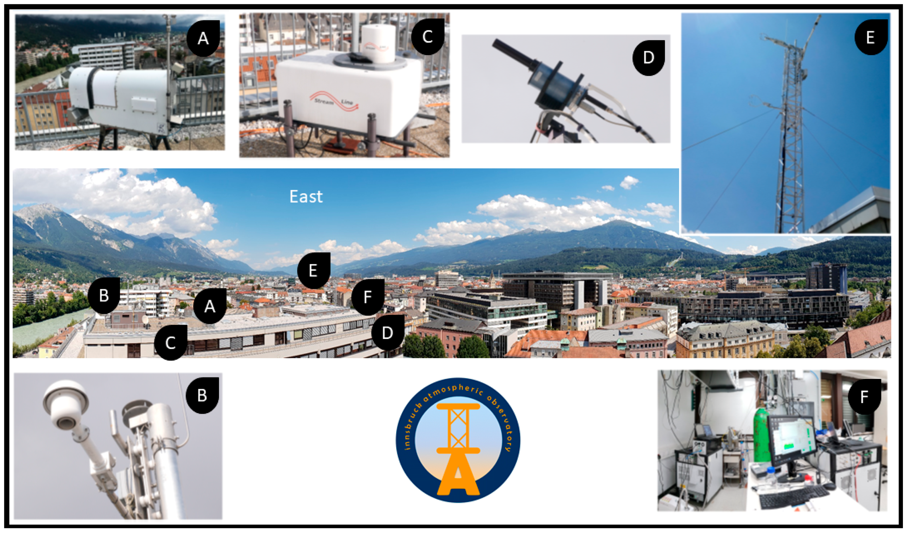
  159. Karl, T.; Gohm, A.; Rotach, M.W.; Ward, H.C.; Graus, M.; Cede, A.; Wohlfahrt, G.; Hammerle, A.; Haid, M.; Tiefengraber, M.; et al. Studying urban climate and air quality in the Alps: The Innsbruck atmospheric observatory. Bull. Amer. Meteor. Soc. 2020, 101, E488–E507. [Google Scholar] [CrossRef] [Green Version]
  160. Monroy, J.G.; Lilienthal, A.J.; Blanco, J.L.; Gonzalez-Jimenez, J.; Trincavelli, M. Probabilistic gas quantification with MOX sensors in open sampling systems—A gaussian process approach. Sens. Actuator B Chem. 2013, 188, 298–312. [Google Scholar] [CrossRef] [Green Version]
  161. Sun, Y.-F.; Liu, S.-B.; Meng, F.-L.; Liu, J.-Y.; Zhen, J.; Kong, L.-T.; Liu, J.-H. Metal oxide nanostructures and their gas sensing properties: A review. Sensors 2012, 12, 2610–2631. [Google Scholar] [CrossRef] [PubMed] [Green Version]
  162. WMO. Low-Cost Sensors for the Measurement of Atmospheric Composition: Overview of Topic and Future Applications; World Meteorological Organization: Geneva, Switzerland, 2018; p. 46. [Google Scholar]
  163. Cavaliere, A.; Carotenuto, F.; Di Gennaro, F.; Gioli, B.; Gualtieri, G.; Martelli, F.; Matese, A.; Toscano, P.; Vagnoli, C.; Zaldei, A. Development of low-cost air quality atations for next generation monitoring networks: Calibration and validation of PM2.5 and PM10 sensors. Sensors 2018, 18, 2843. [Google Scholar] [CrossRef] [PubMed] [Green Version]
  164. Althausen, D.; Engelmann, R.; Baars, H.; Heese, B.; Ansmann, A.; Müller, D.; Komppula, M. Portable Raman Lidar PollyXT for automated profiling of aerosol backscatter, extinction, and depolarization. J. Atmos. Ocean. Technol. 2009, 26, 2366–2378. [Google Scholar] [CrossRef]
  165. Harnish, F.; Gohm, A.; Fix, A.; Schnitzhofer, R.; Hansel, A.; Neininger, B. Spatial distribution of aerosols in the Inn Valley atmosphere during wintertime. Meteorol. Atmos. Phys. 2009, 103, 223–235. [Google Scholar] [CrossRef] [Green Version]
  166. Meister, A.; Fix, A.; Flentje, H.; Wirth, M.; Ehret, G. TropOLEX: A new tuneable airborne lidar system for the measurement of tropospheric ozone. In Proceedings of the 6th International Symposium on Tropospheric Profiling, Leipzig, Germany, 14–20 September 2003. [Google Scholar]
  167. Chazette, P.; Couvert, P.; Randriamiarisoa, H.; Sanak, J.; Bonsang, B.; Moral, P.; Berthier, S.; Salanave, S.; Toussaint, F. Three-dimensional survey of pollution during winter in French Alps valleys. Atmos. Environ. 2005, 39, 35–47. [Google Scholar] [CrossRef]
  168. Kreher, K.; van Roozendael, M.; Hendrick, F.; Apituley, A.; Dimitropoulou, E.; Frieß, U.; Richter, A.; Wagner, T.; Lampel, J.; Abuhassan, N.; et al. Intercomparison of NO2, O4, O3 and HCHO slant column measurements by MAX-DOAS and zenith-sky UV–visible spectrometers during CINDI-2. Atmos. Meas. Tech. 2020, 13, 2169–2208. [Google Scholar] [CrossRef]
  169. Schreier, S.F.; Richter, A.; Wittrock, F.; Burrows, J.P. Estimates of free-tropospheric NO2 and HCHO mixing ratios derived from high-altitude mountain MAX-DOAS observations at midlatitudes and in the tropics. Atmos. Chem. Phys. 2016, 16, 2803–2817. [Google Scholar] [CrossRef] [Green Version]
  170. Emeis, S.; Kalthoff, N.; Adler, B.; Pardyjak, E.; Paci, A.; Junkermann, W. High-resolution observations of transport and exchange processes in mountainous terrain. Atmosphere 2018, 9, 457. [Google Scholar] [CrossRef] [Green Version]
  171. Tomasi, E.; Giovannini, L.; Falocchi, M.; Zardi, D.; Antonacci, G. Preliminary pollutant dispersion modelling with CALMET and CALPUFF over complex terrain in the Bolzano Basin (IT). In Proceedings of the HARMO 2016—17th International Conference on Harmonisation within Atmospheric Dispersion Modelling for Regulatory Purposes, Budapest, Hungary, 9–12 May 2016; Ferenczi, Z., Bozo, L., Puskas, M.T., Eds.; Hungarian Meteorological Service: Budapest, Hungary, 2016; pp. 160–164. [Google Scholar]
  172. Haiden, T.; Kann, A.; Wittmann, C.; Pistotnik, G.; Bica, B.; Gruber, C. The integrated nowcasting through comprehensive analysis (INCA) system and its validation over the eastern Alpine region. Weather Forecast. 2011, 26, 166–183. [Google Scholar] [CrossRef]
  173. Hacker, J.; Draper, C.; Madaus, L. Challenges and opportunities for data assimilation in mountainous environments. Atmosphere 2018, 9, 127. [Google Scholar] [CrossRef] [Green Version]
  174. Chow, F.K.; Weigel, A.P.; Street, R.L.; Rotach, M.W.; Xue, M. High-resolution large-eddy simulations of flow in a steep Alpine valley. Part I: Methodology, verification, and sensitivity experiments. J. Appl. Meteorol. Climatol. 2006, 45, 63–86. [Google Scholar] [CrossRef] [Green Version]
  175. Skamarock, W.C. Evaluating mesoscale NWP models using kinetic energy spectra. Mon. Weather Rev. 2004, 132, 3019–3032. [Google Scholar] [CrossRef]
  176. Giovannini, L.; Antonacci, G.; Zardi, D.; Laiti, L.; Panziera, L. Sensitivity of simulated wind speed to spatial resolution over complex terrain. Energy Proced. 2014, 59, 323–329. [Google Scholar] [CrossRef] [Green Version]
  177. Shicker, I.; Seibert, P. Simulation of the meteorological conditions during a winter smog episode in the Inn Valley. Meteorol. Atmos. Phys. 2009, 103, 211–222. [Google Scholar] [CrossRef]
  178. Trini Castelli, S.; Morelli, S.; Anfossi, D.; Carvalho, J.; Zauli Sajani, S. Intercomparison of two models, ETA and RAMS, with TRACT field campaign data. Environ. Fluid Mech. 2004, 4, 157–196. [Google Scholar] [CrossRef]
  179. Balanzino, A.; Trini Castelli, S. Numerical experiments with RAMS model in highly complex terrain. Environ. Fluid Mech. 2018, 18, 357–381. [Google Scholar] [CrossRef]
  180. Wyngaard, J.C. Toward numerical modeling in the “terra incognita”. J. Atmos. Sci. 2004, 61, 1816–1826. [Google Scholar] [CrossRef]
  181. Chow, F.K.; Schar, C.; Ban, N.; Lundquist, K.A.; Schlemmer, L.; Shi, X. Crossing multiple gray zones in the transition from mesoscale to microscale simulation over complex terrain. Atmosphere 2019, 10, 274. [Google Scholar] [CrossRef] [Green Version]
  182. Muñoz-Esparza, D.; Sauer, J.A.; Linn, R.R. Limitations of one-dimensional mesoscale PBL parameterizations in reproducing mountain-wave flows. J. Atmos. Sci. 2016, 73, 2603–2614. [Google Scholar] [CrossRef]
  183. Goger, B.; Rotach, M.W.; Gohm, A.; Fuhrer, O.; Stiperski, I.; Holtslag, A.A.M. The impact of 3D effects on the simulation of turbulence kinetic energy structure in a major Alpine valley. Bound. Layer Meteorol. 2018, 168, 1–27. [Google Scholar] [CrossRef] [PubMed] [Green Version]
  184. Łobocki, L. Surface-layer flux–gradient relationships over inclined terrain derived from a local equilibrium, turbulence closure model. Bound. Layer Meteorol. 2014, 150, 469–483. [Google Scholar] [CrossRef] [Green Version]
  185. Trini Castelli, S.; Ferrero, E.; Anfossi, D.; Ying, R. Comparison of turbulence closure models over a schematic valley in a neutral boundary layer. In Proceedings of the 13th Symposium on Boundary Layers and Turbulence, Dallas, TX, USA, 10–15 January 1999. [Google Scholar]
  186. Trini Castelli, S.; Ferrero, E.; Anfossi, D. Turbulence closures in neutral boundary layer over complex terrain. Bound. Layer Meteorol. 2001, 100, 405–419. [Google Scholar] [CrossRef]
  187. Ferrero, E.; Colonna, N. Nonlocal treatment of the buoyancy-shear-driven boundary layer. J. Atmos. Sci. 2006, 63, 2653–2662. [Google Scholar] [CrossRef]
  188. Canuto, V.; Howard, A.; Cheng, Y.; Dubovikov, M. Ocean turbulence, part II: Vertical diffusivities of momentum, heat, salt, mass and passive scalars. J. Phys. Oceanogr. 2002, 32, 240–264. [Google Scholar] [CrossRef]
  189. Gryanik, V.; Hartmann, J.; Raasch, S.; Schoroter, M. A refinement of the Millionschikov quasi-normality hypothesis for convective boundary layer turbulence. J. Atmos. Sci. 2005, 62, 2632–2638. [Google Scholar] [CrossRef]
  190. Colonna, N.M.; Ferrero, E.; Rizza, U. Nonlocal boundary layer: The pure buoyancy-driven and the buoyancy-shear-driven cases. J. Geophys. Res. Atmos. 2009, 114, 148–227. [Google Scholar] [CrossRef] [Green Version]
  191. Canuto, V. Turbulent convection with overshootings: Reynolds stress approach. Astrophys. J. 1992, 392, 218–232. [Google Scholar] [CrossRef]
  192. Ferrero, E.; Racca, M. The role of the non-local transport in modelling the shear-driven atmospheric boundary layer. J. Atmos. Sci. 2004, 61, 1434–1445. [Google Scholar] [CrossRef]
  193. Ferrero, E.; Alessandrini, S.; Vandenberghe, F. Assessment of planetary-boundary-layer schemes in the Weather Research and Forecasting model within and above an urban canopy layer. Bound. Layer Meteorol. 2018, 168, 289–319. [Google Scholar] [CrossRef]
  194. Cuxart, J. When can a high-resolution simulation over complex terrain be called LES? Front. Earth Sci. 2015, 3, 87. [Google Scholar] [CrossRef] [Green Version]
  195. Tomasi, E.; Giovannini, L.; Zardi, D.; de Franceschi, M. Optimization of Noah and Noah_MP land surface schemes in snow-melting conditions over complex terrain. Mon. Weather Rev. 2017, 145, 4727–4745. [Google Scholar] [CrossRef]
  196. Foster, C.S.; Crosman, E.T.; Horel, J.D. Simulations of a cold-air pool in Utah’s Salt Lake Valley: Sensitivity to land use and snow cover. Bound. Layer Meteorol. 2017, 164, 1–25. [Google Scholar] [CrossRef]
  197. Jiménez-Esteve, B.; Udina, M.; Soler, M.R.; Pepin, N.; Miró, J.R. Land use and topography influence in a complex terrain area: A high resolution mesoscale modelling study over the Eastern Pyrenees using the WRF model. Atmos. Res. 2018, 202, 49–62. [Google Scholar] [CrossRef] [Green Version]
  198. Massey, J.D.; Steenburgh, W.J.; Knievel, J.C.; Cheng, W.Y.Y. Regional soil moisture biases and their influence on WRF model temperature forecasts over the Intermountain West. Weather Forecast. 2016, 31, 197–216. [Google Scholar] [CrossRef]
  199. Ookouchi, Y.; Segal, M.; Kessler, R.C.; Pielke, R.A. Evaluation of soil moisture effects on the generation and modification of mesoscale circulations. Mon. Weather Rev. 1984, 112, 2281–2292. [Google Scholar] [CrossRef] [Green Version]
  200. Maggioni, V.; Houser, P.R. Soil moisture data assimilation. In Data Assimilation for Atmospheric, Oceanic and Hydrologic Applications; Park, S., Xu, L., Eds.; Springer: Cham, Switzerland, 2017; Volume 3, pp. 195–217. [Google Scholar]
  201. Chen, F.; Manning, K.W.; LeMone, M.A.; Trier, S.B.; Alfieri, J.G.; Roberts, R.; Tewari, M.; Niyogi, D.; Horst, T.W.; Oncley, S.P.; et al. Description and evaluation of the characteristics of the NCAR high-resolution land data assimilation system. J. Appl. Meteor. Climatol. 2007, 46, 694–713. [Google Scholar] [CrossRef] [Green Version]
  202. Giuseppe, F.D.; Cesari, D.; Bonafé, G. Soil initialization strategy for use in limited-area weather prediction systems. Mon. Weather. Rev. 2011, 139, 1844–1860. [Google Scholar] [CrossRef]
  203. Angevine, W.M.; Bazile, E.; Legain, D.; Pino, D. Land surface spinup for episode modeling. Atmos. Chem. Phys. 2014, 14, 8165–8172. [Google Scholar] [CrossRef] [Green Version]
  204. Maxwell, R.M.; Chow, F.K.; Kollet, S.J. The groundwater-land-surface-atmosphere connection: Soil moisture effects on the atmospheric boundary layer in fully-coupled simulations. Adv. Water Resour. 2007, 30, 2447–2466. [Google Scholar] [CrossRef] [Green Version]
  205. Rihani, J.F.; Chow, F.K.; Maxwell, R.M. Isolating effects of terrain and soil moisture heterogeneity on the atmospheric boundary layer: Idealized simulations to diagnose land-atmosphere feedbacks. J. Adv. Model. Earth Syst. 2015, 7, 915–937. [Google Scholar] [CrossRef]
  206. Zhong, J.; Lu, B.; Wang, W.; Huang, C.; Yang, Y. Impact of soil moisture on winter 2-m temperature forecast in Northern China. J. Hydrometeor. 2020, 21, 597–614. [Google Scholar] [CrossRef]
  207. Rummler, T.; Arnault, J.; Gochis, D.; Kunstmann, H. Role of lateral terrestrial water flow on the regional water cycle in a complex terrain region: Investigation with a fully coupled model system. J. Geophys. Res. Atmos. 2019, 124, 507–529. [Google Scholar] [CrossRef]
  208. Barlage, M.; Chen, F.; Tewari, M.; Ikeda, K.; Gochis, D.; Dudhia, J.; Rasmussen, R.; Livneh, B.; Ek, M.; Mitchell, K. Noah land surface model modifications to improve snowpack prediction in the Colorado Rocky Mountains. J. Geophys. Res. Atmos. 2010, 115, D22101. [Google Scholar] [CrossRef] [Green Version]
  209. Jin, J.; Miller, N.L.; Schlegel, N. Sensitivity study of four land surface schemes in the WRF Model. Adv. Meteor. 2010, 2010, 167436. [Google Scholar] [CrossRef] [Green Version]
  210. Hall, D.K.; Riggs, G.A.; Salomonson, V.V. MODIS/Terra Snow Cover 5-Min L2 Swath 500m, Version 5; NASA National Snow and Ice Data Center Distributed Active Archive Center: Boulder, CO, USA, 2006.
  211. Chen, F.; Kusaka, H.; Bornstein, R.; Ching, J.; Grimmond, C.S.B.; Grossman-Clarke, S.; Loridan, T.; Manning, K.W.; Martilli, A.; Miao, S.; et al. The integrated WRF/urban modelling system: Development, evaluation, and applications to urban environmental problems. Int. J. Climatol. 2011, 31, 273–288. [Google Scholar] [CrossRef]
  212. Ching, J.; Brown, M.; Burian, S.; Chen, F.; Cionco, R.; Hanna, A.; Hultgren, T.; McPherson, T.; Sailor, D.; Taha, H.; et al. National urban database and access portal tool. Bull. Amer. Meteor. Soc. 2009, 90, 1157–1168. [Google Scholar] [CrossRef] [Green Version]
  213. Goger, B.; Rotach, M.W.; Gohm, A.; Stiperski, I.; Fuhrer, O.; de Morsier, G. A new horizontal length scale for a three-dimensional turbulence parameterization in meso-scale atmospheric modeling over highly complex terrain. J. Appl. Meteorol. Climatol. 2019, 58, 2087–2102. [Google Scholar] [CrossRef]
  214. Rotach, M.W.; Gryning, S.E.; Tassone, C. A two-dimensional stochastic Lagrangian dispersion model for daytime conditions. Q. J. R. Meteorol. Soc. 1996, 122, 367–389. [Google Scholar] [CrossRef]
  215. Hanna, S. Applications in air pollution modeling. In Atmospheric Turbulence and Air Pollution Modelling; Nieuwstadt, F., van Dop, H., Eds.; Reidel: Dordrecht, The Netherlands, 1982; pp. 275–310. [Google Scholar]
  216. Trini Castelli, S.; Tinarelli, G.; Reisin, T.G. Comparison of atmospheric modelling systems simulating the flow, turbulence and dispersion at the microscale within obstacles. Environ. Fluid Mech. 2017, 17, 879–901. [Google Scholar] [CrossRef]
  217. Thomson, D.J. Criteria for the selection of stochastic models of particle trajectories in turbulent flows. J. Fluid Mech. 1987, 180, 529–556. [Google Scholar] [CrossRef]
  218. Luhar, A.K.; Britter, R.E. A random walk model for dispersion in inhomogeneous turbulence in a convective boundary layer. Atmos. Environ. 1989, 23, 1911–1924. [Google Scholar] [CrossRef]
  219. Flesch, T.K.; Wilson, J.D. A two-dimensional trajectory-simulation model for non-Gaussian, inhomogeneous turbulence within plant canopies. Bound. Layer Meteorol. 1992, 61, 349–374. [Google Scholar] [CrossRef]
  220. Monti, P.; Leuzzi, G. A closure to derive a three-dimensional well-mixed trajectory model for non-Gaussian, inhomogeneous turbulence. Bound. Layer Meteorol. 1996, 80, 311–331. [Google Scholar] [CrossRef]
  221. Wilson, J.D.; Flesch, T.K. Trajectory curvature as a selection criterion for valid Lagrangian stochastic dispersion models. Bound. Layer Meteorol. 1997, 84, 411–425. [Google Scholar] [CrossRef]
  222. Sawford, B.L. Rotation of trajectories in Lagrangian stochastic models of turbulent dispersion. Bound. Layer Meteorol. 1999, 93, 411–424. [Google Scholar] [CrossRef]
  223. Kurbanmuradov, O.; Sabelfeld, K. Lagrangian stochastic models for turbulent dispersion in the atmospheric boundary layer. Bound. Layer Meteorol. 2000, 97, 191–218. [Google Scholar] [CrossRef]
  224. Stein, A.F.; Lamb, D.; Draxler, R.R. Incorporation of detailed chemistry into a three-dimensional Lagrangian–Eulerian hybrid model: Application to regional tropospheric ozone. Atmos. Environ. 2000, 34, 4361–4372. [Google Scholar] [CrossRef]
  225. Alessandrini, S.; Ferrero, E. A hybrid Lagrangian–Eulerian particle model for reacting pollutant dispersion in non-homogeneous non-isotropic turbulence. Phys. A 2009, 388, 1375–1387. [Google Scholar] [CrossRef]
  226. Alessandrini, S.; Ferrero, E. A Lagrangian particle model with chemical reactions: Application in real atmosphere. Int. J. Environ. Pollut. 2011, 47, 97–107. [Google Scholar] [CrossRef] [Green Version]
  227. Kaplan, H. An estimation of a passive scalar variances using a one-particle Lagrangian transport and diffusion model. Phys. A 2014, 393, 1–9. [Google Scholar] [CrossRef]
  228. Ferrero, E.; Mortarini, L.; Alessandrini, S.; Lacagnina, C. Application of a bivariate gamma distribution for a chemically reacting plume in the atmosphere. Bound. Layer Meteorol. 2013, 147, 123–137. [Google Scholar] [CrossRef]
  229. Amicarelli, A.; Leuzzi, G.; Monti, P.; Alessandrini, S.; Ferrero, E. A stochastic Lagrangian micromixing model for the dispersion of reactive scalars in turbulent flows: Role of concentration fluctuations and improvements to the conserved scalar theory under non-homogeneous conditions. Environ. Fluid Mech. 2017, 17, 715–753. [Google Scholar] [CrossRef]
  230. Ferrero, E.; Mortarini, L.; Alessandrini, S.; Lacagnina, C. A fluctuating plume model for pollutants dispersion with chemical reactions. Int. J. Environ. Pollut. 2012, 48, 3–12. [Google Scholar] [CrossRef]
  231. Garmory, A.; Richardson, E.S.; Mastorakos, E. Micromixing effects in a reacting plume by the stochastic fields method. Atmos. Environ. 2006, 40, 1078–1091. [Google Scholar] [CrossRef]
  232. Luhar, A.; Hibberd, M.; Borgas, M. A skewed meandering-plume model for concentration statistics in the convective boundary layer. Atmos. Environ. 2000, 34, 3599–3616. [Google Scholar] [CrossRef]
  233. Franzese, P. Lagrangian stochastic modeling of a fluctuating plume in the convective boundary layer. Atmos. Environ. 2003, 37, 1691–1701. [Google Scholar] [CrossRef]
  234. Mortarini, L.; Franzese, P.; Ferrero, E. A fluctuating plume model for concentration fluctuations in a plant canopy. Atmos. Environ. 2009, 43, 921–927. [Google Scholar] [CrossRef]
  235. Bisignano, A.; Mortarini, L.; Ferrero, E.; Alessandrini, S. Analytical offline approach for concentration fluctuations and higher order concentration moments. Int. J. Environ. Pollut. 2014, 5, 58–66. [Google Scholar] [CrossRef]
  236. Manor, A. A stochastic single particle lagrangian model for the concentration fluctuation in a plume dispersing inside an urban canopy. Bound. Layer Meteorol. 2014, 150, 327–340. [Google Scholar] [CrossRef]
  237. Ferrero, E.; Mortarini, L.; Purghè, F. A simple parameterization for the concentration variance dissipation in a Lagrangian single-particle model. Bound. Layer Meteorol. 2017, 163, 91–101. [Google Scholar] [CrossRef]
  238. Tinarelli, G.; Anfossi, D.; Brusasca, G.; Ferrero, E.; Giostra, U.; Morselli, M.G.; Moussafir, J.; Tampieri, F.; Trombetti, F. Lagrangian particle simulation of tracer dispersion in the lee of a schematic two-dimensional hill. J. Appl. Meteorol. 1994, 33, 744–756. [Google Scholar] [CrossRef] [Green Version]
  239. Alessandrini, S.; Ferrero, E.; Trini Castelli, S.; Anfossi, D. Influence of turbulent closure on the simulation of flow and dispersion in complex terrain. Int. J. Environ. Pollut. 2005, 24, 154–170. [Google Scholar] [CrossRef]
  240. Balanzino, A.; Pirovano, G.; Ferrero, E.; Causà, M.; Riva, G.M. Particulate matter pollution simulations in complex terrain. Int. J. Environ. Pollut. 2012, 48, 39–46. [Google Scholar] [CrossRef]
  241. Ferrero, E.; Trini Castelli, S.; Anfossi, D. Turbulence fields for atmospheric dispersion models in horizontally non-homogeneous conditions. Atmos. Environ. 2003, 37, 2305–2315. [Google Scholar] [CrossRef]
  242. Brusasca, G.; Tinarelli, G.; Anfossi, D. Particle model simulation of diffusion in low wind speed stable conditions. Atmos. Environ. 1992, 26, 707–723. [Google Scholar] [CrossRef]
  243. Oettl, D.; Almbauer, R.A.; Sturm, P.J. A new method to estimate diffusion in stable, low wind conditions. J. Appl. Meteorol. 2001, 40, 259–268. [Google Scholar] [CrossRef]
  244. Anfossi, D.; Alessandrini, S.; Trini Castelli, S.; Ferrero, E.; Oettl, D.; Degrazia, G. Tracer dispersion simulation in low wind speed conditions with a new 2-D Langevin equation system. Atmos. Environ. 2006, 40, 7234–7245. [Google Scholar] [CrossRef]
  245. Luhar, A.K.; Hurley, P.J. Application of a coupled prognostic model to turbulence and dispersion in light-wind stable conditions, with an analytical correction to vertically resolve concentrations near the surface. Atmos. Environ. 2012, 5, 56–66. [Google Scholar] [CrossRef]
  246. Luhar, A.K. Lagrangian particle modeling of dispersion in light winds. In Dispersion Lagrangian Modeling of the Atmosphere; Lin, J.C., Brunner, D., Gerbig, C., Stohl, A., Luhar, A., Webley, P., Eds.; American Geophysical Union: Washington, DC, USA, 2012; pp. 311–328. [Google Scholar]
  247. Pouliot, G.; Pierce, T.; Benjey, W.; O’Neill, S.M.; Ferguson, S.A. Wildfire emission modeling: Integrating bluesky and smoke. In Proceedings of the 14th International Emission Inventory Conference “Transforming Emission Inventories Meeting Future Challenges Today”, Las Vegas, NV, USA, 11–14 April 2005. [Google Scholar]
  248. Briggs, G.A. Plume rise predictions. In Lectures on Air Pollution and Environmental Impact Analyses. Workshop Proceedings; Haugen, D., Ed.; American Meteorological Society: Boston, Massachusetts, MA, USA, 1975; pp. 59–111. [Google Scholar]
  249. Weil, J.; Snyder, W.; Lawson, R., Jr.; Shipman, M. Experiments on buoyant plume dispersion in a laboratory convection tank. Bound. Layer Meteorol. 2002, 102, 367–414. [Google Scholar] [CrossRef]
  250. Morton, B.R.; Taylor, G.I.; Turner, J.S. Turbulent gravitational convection from maintained and instantaneous sources. Proc. Roy. Soc. London. 1956, A234, 1–23. [Google Scholar]
  251. Anfossi, D.; Ferrero, E.; Brusasca, G.; Marzorati, A.; Tinarelli, G. A simple way of computing buoyant plume rise in a Lagrangian stochastic model for airborne dispersion. Atmos. Environ. 1993, 27A, 1443–1451. [Google Scholar] [CrossRef]
  252. Webster, H.N.; Thomson, D.J. Validation of a Lagrangian model plume rise scheme using the Kincaid data set. Atmos. Environ. 2002, 36, 5031–5042. [Google Scholar] [CrossRef]
  253. Alessandrini, S.; Ferrero, E.; Anfossi, D. A new Lagrangian method for modelling the buoyant plume rise. Atmos. Environ. 2013, 77, 239–249. [Google Scholar] [CrossRef]
  254. Oettl, D.; Ferrero, E. A simple model to assess odour hours for regulatory purposes. Atmos. Environ. 2017, 155, 162–173. [Google Scholar] [CrossRef]
  255. Ferrero, E.; Alessandrini, S.; Anderson, B.; Tomasi, E.; Jiménez, P.; Meech, S. Lagrangian simulation of smoke plume from fire and validation using ground-based lidar and aircraft measurements. Atmos. Environ. 2019, 213, 659–674. [Google Scholar] [CrossRef]
  256. Thomson, D.J. A stochastic model for the motion of particle pairs in isotropic high-Reynolds-number turbulence, and its application to the problem of concentration variance. J. Fluid Mech. 1990, 210, 113–153. [Google Scholar] [CrossRef]
  257. Borgas, M.S.; Sawford, B.L. A family of stochastic models for particle dispersion in isotropic homogeneous stationary turbulence. J. Fluid Mech. 1994, 279, 69–99. [Google Scholar] [CrossRef]
  258. Pope, S. PDF methods for turbulent reactive flows. Prog. Energy Combust. Sci. 1985, 11, 119–192. [Google Scholar] [CrossRef]
  259. Cassiani, M.; Franzese, P.; Giostra, U. A PDF micromixing model of dispersion for atmospheric flow. Part I: Development of the model, application to homogeneous turbulence and to neutral boundary layer. Atmos. Environ. 2005, 39, 1457–1469. [Google Scholar] [CrossRef]
  260. Yee, E.; Chan, R.; Kosteniuk, P.R.; Chandler, G.M.; Biltoft, C.A.; Bowers, J.F. Incorporation of internal fluctuations in a meandering plume model of concentration fluctuations. Bound. Layer Meteorol. 1994, 67, 11–38. [Google Scholar] [CrossRef]
  261. Yee, E.; Wilson, D.J. A comparison of the detailed structure in dispersing tracer plumes measured in grid-generated turbulence with a meandering plume model incorporating internal fluctuations. Bound. Layer Meteorol. 2000, 94, 253–296. [Google Scholar] [CrossRef]
  262. Ferrero, E.; Oettl, D. An evaluation of a Lagrangian stochastic model for the assessment of odours. Atmos. Environ. 2019, 206, 237–246. [Google Scholar] [CrossRef]
  263. Ferrero, E.; Manor, A.; Mortarini, L.; Oettl, D. Concentration fluctuations and odor dispersion in Lagrangian models. Atmosphere 2020, 11, 27. [Google Scholar] [CrossRef] [Green Version]
Figure 1. Annual emissions of (a) PM10 and (b) NOx in South Tyrol, in the Italian Alps, during 2013, along with height contour lines. Adapted from [5].
Atmosphere 11 00646 g001
Figure 2. Cross sections of tracer concentrations (color contours) after 6 h of simulation for (a) flat terrain and (b) idealized topography, from Lang et al. [35]. The height of the convective boundary layer is plotted according to different definitions: black solid line (potential temperature gradient > 0.001 K m−1), dashed line (Richardson number > 0.25, following [37]), dotted line (Richardson number > 0.25, following [31]), and green solid line (maximum gradient of the tracer). Potential temperature is shown as black contour lines (0.25 K increment). Adapted from [35].
Atmosphere 11 00646 g002
Figure 3. Wind speed measured by a SODAR (SOnic Detection And Ranging) (color contours) in the Adige Valley close to the town of Aldeno in the period 10–19 February 2006 in the framework of the ALPNAP project [11], along with PM10 concentrations (black line) measured at the same site.
Atmosphere 11 00646 g003
Figure 4. Ground level concentrations of a tracer released by a chimney in the Adige Valley (Italy) at different times, calculated by simulations with CALPUFF (left column) and SPRAY-WEB (right column). Adapted from [14].
Atmosphere 11 00646 g004
Figure 5. View of the Innsbruck Atmospheric Observatory (IAO) facilities: (A): microwave sounder, (B) TAWES (The New Austrian Meteorological Measuring Network) weather station, (C) Doppler wind lidar system, (D) Pandora, (E) flux tower, and (F) laboratory facilities.
Atmosphere 11 00646 g005

