Global Warming Potential (GWP) for Methane: Monte Carlo Analysis of the Uncertainties in Global Tropospheric Model Predictions

Abstract

Estimates of the global warming potential (GWP) of methane rely on the predictions from global chemistry-transport models. These models employ many uncertain input parameters representing the sources and sinks for methane and those for the tropospheric ozone, which is formed as a by-product of the methane sink process. Five thousand quasi-randomly Monte Carlo sampled model runs employing a zonally averaged global model were completed, each with a base case and a pulse case that differed from the base case only in having an additional 149 Tg (1Tg = 10⁹ kg) emission pulse of methane. Each of the five thousand pulse case experiments had a small excess of methane that decayed away throughout the twenty-year model experiment. The radiative forcing consequences of this excess methane, and the excess tropospheric ozone formed from it, were integrated over a 100-year time horizon. The GWP was calculated in each of the five thousand model experiments from the sum of the radiative forcing consequences of methane and tropospheric ozone, by expressing them relative to the radiative forcing consequences of an identical emission pulse of carbon dioxide. The 2-sigma confidence range surrounding the methane atmospheric lifetime estimated in the Monte Carlo analysis was considerably wider than that derived from observations, suggesting that some of the input parameter combinations may have been unrealistic. The rejection of the unrealistic Monte Carlo replicates increased the mean methane GWP and narrowed its 2-sigma confidence interval to 37 ± 10 over a 100-year time horizon for emission pulses of the order of 1 Tg. Multiple linear regression was used to attribute the uncertainty in the output GWPs to each of the 183 uncertain input parameters, which represented emission source sectors, chemical kinetic rate coefficients, dry deposition velocities and biases in temperature and water vapour concentrations. Overall, the only significant contributions to the uncertainty in the methane GWP came from the chemical kinetic parameters representing the CH₄ + OH, CH₃O₂ + HO₂, CH₃O₂ + NO and the terpene + O₃ reaction rate coefficients.

1. Introduction

It has long been recognised that methane (CH₄) is the second most important anthropogenic greenhouse gas after carbon dioxide (CO₂) [1]. CH₄ has significant anthropogenic and natural sources and features in the basket of trace gases that come under the control of the United Nations Framework Convention on Climate Change (UN FCCC) [2]. CH₄ sources have elevated pre-industrial levels [3] from 720–740 ppb (where 1 ppb = 1 nmol CH₄ mol⁻¹ air when expressed as mole fraction or mixing ratio) to present day levels of 1800 ppb. These man-made sources include oil and gas operations, coal mining, natural gas leakage, landfills and enteric fermentation in livestock [4]. The main atmospheric removal processes for CH₄ is its oxidation by hydroxyl (OH) radicals [5,6]. This chemical reaction has a significant temperature coefficient, which means that the sink is concentrated in the warmer, more moist, lower troposphere. The atmospheric lifetime from this oxidation process is of the order of ten years. There are weaker sinks from soil uptake (160 years) and stratospheric OH oxidation (120 years) [4]. The CH₄ oxidation sink also acts as a source of tropospheric ozone (O₃), another important greenhouse gas [1].

The CH₄ oxidation sink involving OH radicals not only controls the CH4 atmospheric lifetime and hence the CH₄ burden but is also an important process controlling the fast, photochemical balance of the troposphere. In fact, it is so important that increasing CH₄ burdens reduce the OH radical steady state concentration and extend the atmospheric lifetime. Increasing CH₄ burdens therefore effectively reduces their own sink strength, leading to a positive feedback or amplification [4]. Consequently, CH₄ is a direct greenhouse gas by virtue of its infrared absorption spectrum and an indirect greenhouse gas because it is able to perturb its own tropospheric distribution and that of tropospheric O₃, the third most important anthropogenic greenhouse gas after CO₂ and CH₄ [1].

There have been a number of studies on the direct and radiative forcing consequences of CH₄ emissions and these have been kept under review by the Intergovernmental Panel on Climate Change. A convenient metric defining and quantifying these radiative forcing consequences is the Global Warming Potential (GWP) [7]. Over a 100-year time horizon, CH4 has a GWP of about 30 [1], that is to say, the time-integrated radiative forcing consequences of an emission of 1 Tg of CH₄ is equivalent to the emission of 30 Tg of CO2. The GWP concept has, however, been criticised because it does not represent climate policy temperature goals [8] and other metrics have been proposed [9]. However, the aim of this study is to address the radiative forcing consequences of CH₄ emissions and so the GWP metric will suffice as an endpoint in our analyses.

Studies on the radiative forcing consequences of anthropogenic CH₄ emissions with global chemistry-transport models employed in the estimation of global warming potentials (GWPs) are not without some singular difficulties that are relevant solely to CH₄. Because of its ten-year atmospheric lifetime, the global CH₄ distribution is not always in steady state with its sources and sinks either in the real atmosphere or within the global chemistry-transport models. The difficulties are such that some global chemistry-transport models use prescribed CH₄ levels, and, in others, relatively short run times are employed. This means that the quantification of CH₄ amplification factors and indirect radiative forcing contributions are surrounded by uncertainties.

This is the third of a three-part study. In the first part [10], a methodology was laid out for a Monte Carlo (MC) analysis of the uncertainties in tropospheric O₃ sources and sinks in a global Lagrangian chemistry-transport model. In the second part [11], this same MC methodology was applied within a zonally averaged coarse resolution global tropospheric O₃ model to investigate the uncertainties in the global burdens and turnovers of CH₄, carbon monoxide (CO) and tropospheric O₃. Here, in the third part, the MC methodology is applied to the investigation of the uncertainties surrounding model estimates of the CH₄ GWP. In this study, the methodological uncertainties surrounding the presence or absence of any steady state between CH₄ sources and sinks have been removed by employing 20-year long model experiments. A Monte Carlo uncertainty analysis has then been completed to investigate where the main uncertainties lie, whether in the atmospheric life cycle of CH₄, in the fast, photochemical balance of the troposphere or in the radiative forcing consequences of atmospheric releases of CH₄. To reduce the computational burden of these global chemistry-transport model experiments, sacrifices have had to be made with the spatial resolution of the modelling tool employed, through the use of a zonally-averaged (latitude-altitude) model. The aim has been to identify where model input uncertainties are likely to be the most significant so that future research efforts can be focused on them to reduce uncertainties in the GWP for CH₄.

2. Monte Carlo Uncertainty Analysis and Its Methodology

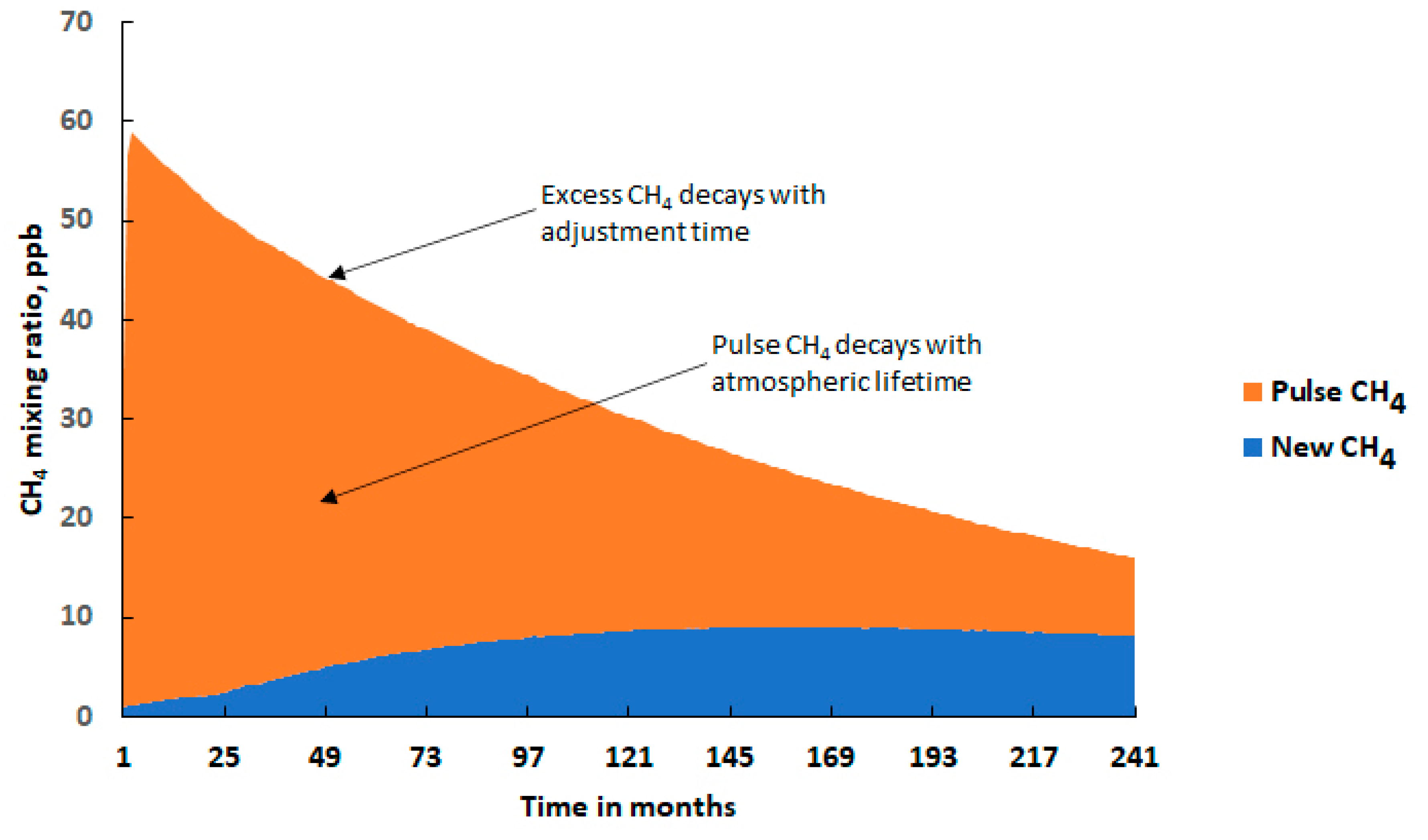
2.1. The Pulse Behaviour of Methane

For a trace gas with a spatially and temporally independent first-order loss process, for example, radioactive decay, integrating over the globe gives the loss rate (L in Tg year⁻¹), which, when divided into the global burden, (B in Tg), gives the atmospheric lifetime or residence time (LT) [12]. If the trace gas is in a steady state, then an instantaneous pulse of the trace gas, A₀, will decay with time, t, according to A = A₀ exp(−k₁t), with an e-folding time constant of the reciprocal of k₁, which is equal to the lifetime, LT.

For CH₄, where the first order loss process is controlled largely by OH radicals and where the OH radical steady state is depleted by increasing CH₄ burdens, a different response is seen to CH₄ perturbations. CH₄ pulses reduce tropospheric OH, which increases the lifetime of the CH₄ pulse and hence amplifies the response [13]. The decay of a CH₄ pulse is thus no longer controlled by the atmospheric lifetime but by a longer time constant, the adjustment time, AT. Therefore, a CH₄ pulse, [CH₄]₀, decays according to: [CH₄] = [CH₄]₀ exp(−k₂t), with an e-folding time constant of AT, which is equal to the reciprocal of k_2. The ratio of the adjustment time to the lifetime depends on the exact formulation of the atmospheric chemistry of CH₄, CO and OH, with values varying between 1.23 and 1.62 [4]. CH₄ has an important chemical feedback that amplifies the impacts of CH₄ perturbations [14]. This feedback or amplification was characterised using a feedback factor (FF), which represents the percentage change in CH₄ loss frequency for a one percent increase in CH₄ burden. Feedback factors have been reported in the range −0.17% to −0.35% [4] and these FF values are related to AT and LT using: AT/LT = 1/(1 + FF). Apparently, the feedback factors are not correlated with the CH₄ lifetimes, suggesting that they do not depend on it, but depend rather on the CH₄, CO and OH chemistry [12].

Pulses of CH₄ lead to an increase in the already existing CH₄ burden, which cannot be distinguished from the pulse itself. Accordingly, the ‘excess’ CH₄ decays away with the adjustment time constant, that is to say: [CH₄]_excess = [CH₄]₀ exp(−k₂t). If the pulse itself had been tagged, then it would be found to decay with the e-folding time of the atmospheric lifetime, that is to say: [CH₄]_pulse = [CH₄]₀.exp(−k₁t). The difference between these two decays is the ‘new’ CH₄, which has been produced by the depletion in the OH radical steady state by CH₄. Accordingly, we can then write: [CH₄]_new = [CH₄]_0.exp(−k₂t) − [CH₄]₀.exp(−k₁t). This ‘new’ CH₄ starts from zero, reaches a maximum and then declines towards zero. The fraction of the time-integrated ‘excess’ CH₄ that is ‘new’ is found to be: 1 − k₂/k₁.

Over the years since the publication of the first Intergovernmental Panel on Climate Change (IPCC) report [7], these definitions have remained largely unchanged, as have the atmospheric lifetimes, adjustment times and feedback factors for CH₄. A formal description of the delayed recovery of a CH₄ perturbation in terms of the eigenvalues and eigenvectors of the coupled tropospheric CH₄, CO and OH atmospheric chemistry system has been provided, together with a formal quantification of the CH₄ adjustment time [15]. CH₄ perturbations have been tracked by following CH₄ perturbation runs minus control runs for up to a decade [16,17]. However, these decadal long chemistry-transport model studies are relatively rare with many global chemistry-transport model studies using fixed CH₄ and CO levels to avoid the need for long model runs. For example, in the Atmospheric Chemistry Coupled Climate Model Intercomparison Project (ACCMIP) study, thirteen out of the fifteen models used fixed CH₄ levels [10].

2.2. TROPOS Model

In the first part of this study [10], the MC methodology was applied within a global Lagrangian chemistry-transport model (CTM), but, because of limited computer resources, a sufficiently large enough number of MC replicates could not be completed. There was not enough statistical power to complete a regression analysis linking model output uncertainty to model input parameter uncertainty. In the second part [11], the MC methodology was applied within the cut-down and fast for the running of the CTM TROPOSpheric O₃ model, and up to 10,000 MC replicates were performed, allowing regression analyses to be performed, linking uncertainties in global burdens and turnovers to TROPOS input uncertainties. Here, the MC methodology is again applied within TROPOS but this time to investigate the uncertainties in the model estimated CH₄ GWP. We begin with a brief description of the TROPOS model to which the MC uncertainty analysis techniques are applied.

TROPOS uses a zonally averaged (altitude–latitude) and coarse resolution approach by averaging along latitude circles and dividing the atmosphere from the Earth’s surface to an altitude of 24 km into 12 km × 2 km layers and 24 latitude bands. A full description of the off-line advection and dispersion processes in TROPOS is available elsewhere [18]. The chemical mechanism in the original TROPOS model was replaced with an extended chemistry scheme (Common Representative Intermediates CRI v2-R5) [19,20]. This chemical scheme implemented here included 51 species that take part in 157 thermal and photochemical reactions. Emissions for a wide-range of trace gases, including 11 organic compounds, arising from anthropogenic, vegetation, biomass burning, lightning, soils and ocean sources, were set up using the global totals from our previous uncertainty study [8]. The TROPOS model equations were integrated using an automatic, accurate numerical integrator (FACSIMILE; [21]). Trace gases were removed from the lowest TROPOS model layer by dry deposition using the same deposition velocity approach as in STOCHEM-MC.

The surface distribution of O₃ in TROPOS was compared with the observations for the year 2000 taken from the International Global Atmospheric Chemistry (IGAC) Tropospheric Ozone Assessment Report (TOAR) review [22]. TROPOS was able to reproduce the relatively constant observed levels found in the Southern Hemisphere, the rise in the mid-latitudes of the Northern Hemisphere peaking around 40–50° N and the fall towards high latitudes. All of the observations fell within the 2-sigma confidence interval calculated from the 5000 MC replicates, except for two sets of observations from the US Pacific marine boundary layer and Cape Matutula, Samoa. This level of agreement between the surface observations and TROPOS was considered satisfactory for the present purpose of studying the uncertainties in the TROPOS estimates of the CH₄ GWP.

2.3. Monte Carlo Uncertainty Analysis

As in the first two parts of this study [10,11], there were three steps in our Monte Carlo assessment of uncertainties. In the first step, the TROPOS model code was altered to accept a multiplier for each model input parameter, scaling the fixed ‘Best Estimate’ value. In the second step, the uncertain input range for each parameter was sampled quasi-randomly and input values were set for the initialisation of a given TROPOS run. In the third step, TROPOS was run repeatedly a large number, typically 5000, of times, with each run having a different quasi-random selection of input parameters. Each TROPOS run returned the tropospheric CH₄ and O₃ burdens, together with the tropospheric CH₄ and O₃ distributions.

A total of 183 TROPOS input parameters were selected for Monte Carlo uncertainty analysis. Of these, 5 represented physical parameters, 34 represented parameters controlling emissions processing, 116 represented thermal chemical kinetic parameters and the remaining 28, photochemical kinetic parameters. Details of these parameters are provided in our previous study [10,11].

For each input parameter, a 3-sigma confidence range was established based on multiplicative scaling by a factor of between 0.65 and 1.35. The probability distribution within that range was taken to be uniformly distributed on either side of the ‘Best Estimate’, that is to say, ‘top hat’ in shape. For temperature, the probability distribution was assumed to be Gaussian, and additive scaling of between −5 K and +5 K was employed. The details of the Monte Carlo methodology are laid out in some detail elsewhere [10,11].

Having set the TROPOS parameter values for the 183 input parameters that control the life cycle of CH₄, O₃ precursor emissions, O₃ formation and sinks, each uncertainty range was sampled quasi-randomly for each TROPOS run. TROPOS was then run many thousands of times, with each particular set of inputs, and the output results were stored. Each different set of inputs generated different CH₄ and O₃ burdens, and tropospheric CH₄ and O₃ distributions. Because the meteorological data were the same in each of the Monte Carlo replicates, small differences in model results could be accurately discerned between the replicates. Each of the 5000 Monte Carlo replicates required two runs of TROPOS. In one run, the ‘base case’ run, the input data were chosen by Monte Carlo sampling. The input data for the second run, the ‘pulse case’ run, differed only from the ‘base case’ in having and emission of 149 Tg of CH₄ during the first month of the twenty-year model experiment. The choice of the 149 Tg CH₄ pulse size, representing a 3% increase in the CH₄ burden, was arbitrary, being small enough to keep the system in its linear range but large enough to produce discernible differences. We demonstrate linearity in Section 3 below and discuss the choice of the number of Monte Carlo replicates below. The Monte Carlo methodology aimed at replacing a single ‘Best Estimate’ TROPOS model run with a set of many thousand TROPOS Monte Carlo replicates, each with slightly different quasi-randomly sampled input data.

Table 1. Monte Carlo uncertainties estimated in this work and in the literature for the burdens and atmospheric lifetimes of tropospheric O₃, CO and CH₄.

	Units	This Study	TROPOS [11]	STOCHEM [10]	ACCMIP [21,24]
O3 burden	Tg	349 ± 101	324 ± 182	374 ± 182	337 ± 46
O3 lifetime	days	22.6 ± 6	20.5 ± 9	23.0 ± 8	22.3 ± 4
CO burden	Tg	484 ± 326	428 ± 253	374 ± 209	323 ± 76
CO lifetime	days	66 ± 36	57 ± 42	53 ± 34	-
CH4 burden	Tg	4842 ± 2230	5195 ± 756	4620 ±460	4813 ± 162
CH4 lifetime	years	11.4 ± 6.4	9.5 ± 4.0	9.0 ± 4.6	9.7 ± 3.0

summarises the results of the Monte Carlo analysis of the uncertainties in the global burdens and atmospheric lifetimes of tropospheric O₃, CO and CH₄ in the ‘base case’ scenarios of the 5000 Monte Carlo replicates in this study. The TROPOS and STOCHEM-MC estimates are based on 10,000 and 98 Monte Carlo replicates, respectively, and are presented in Table 1 for comparison with our previous studies [10,11]. Also presented are the corresponding estimates from the 14 Atmospheric Chemistry Coupled Climate Model Intercomparison Project (ACCMIP) chemistry-climate models [23,24]. Within the 2-sigma confidence limits, none of the differences between this study and the TROPOS and STOCHEM-MC models were found to be statistically significant. The observed estimate [24] of the 1998 atmospheric CH₄ burden of 4950 Tg is close to the present estimate of 4842 ± 2230 Tg, see Table 1. In the present study, the TROPOS and STOCHEM-MC estimates of the CH₄ lifetime are in agreement with that of 11.2 ± 1.3 years based on observations [23]. The observed tropospheric O₃ burden for 2004–2010 is 328 Tg based on the Aura Ozone Monitoring Instrument (OMI) and the Microwave Limb Sounder (MLS) measurements [25]. This value is close to that from the present and previous studies and is well within the two-sigma confidence intervals from STOCHEM-MC. The O₃ turnovers from the present and previous studies were also in close agreement with that of 15.1 ± 3 Tg day⁻¹ from the ACCMIP models [24].

This level of agreement between this study and the other sources quantifying the tropospheric burdens and lifetimes was considered satisfactory for the present purposes of estimating likely uncertainty bounds in the GWP for CH₄. However, an interesting difference was noted between the present study and the TROPOS results in Table 1. It was noted that the two-sigma confidence interval was significantly wider for the present study than for our previous TROPOS and STOCHEM-MC results. This is surprising since both studies used the same model and the same methodology and assumptions for their respective Monte Carlo analyses. The only difference between the studies was the lengths of the model experiments, twenty years in the present case and only three years in TROPOS. Here, the extra length of the model experiments ensured that CH₄ always came into steady state with the model inputs, a situation that was not realised in TROPOS or the other models in Table 1. The extra length of the model experiments meant that CH₄ burdens came into a steady state, with even the least and greatest atmospheric lifetimes, widening the range of the CH₄ burdens to a considerable degree beyond that achieved in TROPOS or the other models. Indeed, the range achieved in the CH₄ burden is considerably beyond that observed, calling into question its validity. We will return to the significance of this unduly wide uncertainty range in the Discussion and Conclusions section, below.

To understand how the uncertainties in each of the 183 model input parameters contributed to the uncertainty in a particular model output, multiple linear regression techniques were applied to the output results from the Monte Carlo replicates. The basic data employed in these regression analyses were the outputs calculated in the TROPOS runs, for example, the GWP for CH₄, and the values of the 183 input scaling parameters, p_1–183, employed in each TROPOS run. Multiple linear regression was then used to express the outputs as functions of the input parameters using Equation (1) of the form:

GWP = a₁p₁ + a₂p₂ + a₃p₃+ … + a₁₈₃p₁₈₃

(1)

where a₁–a₁₈₃ represent the slopes of the regression. The software package (PV-WAVE, Visual Numerics, Boulder, CO, USA) also returned the fraction of the variance in the GWP that was accounted for by all the p₁–p₁₈₃ taken together and by the parameters individually. Much of the analysis presented here uses the partial correlation coefficients, R_1–183, of the GWP on the individual parameters, p₁–p₁₈₃.

Multiple linear regression assumes that parameters are normally distributed and independent, and there are some issues with this approach when these assumptions are not always found to be the case. However, in this application, multiple regression is used merely as a screening tool to indicate in which broad area the main uncertainties in the CH₄ GWP arise, whether in the emissions, atmospheric chemistry, meteorology or physical parameterisations. Multiple regression is a widely used approach in the literature to understand the uncertainties in chemistry-transport models [26,27,28].

An important issue to establish from the outset is the number of Monte Carlo replicates to be performed. Because the aim of the study is to attribute the uncertainties in TROPOS model outputs to model inputs, an adequate number of replicates is required to be able to conduct multiple linear regression. Since we have identified 183 uncertain model inputs, this fixes the minimum number of replicates. The more replicates we have over and above this minimum, the greater the statistical power in the multiple linear regression. A multiple linear regression was conducted using the tropospheric O₃ burden as output, beginning with 500 Monte Carlo replicates and then moving up in stages. We found that up to 5000 replicates were required before partial correlation coefficients settled down to within ± 10% and ceased changing with increasing numbers of replicates. On this basis, the number of 5000 replicates was chosen in subsequent Monte Carlo analyses.

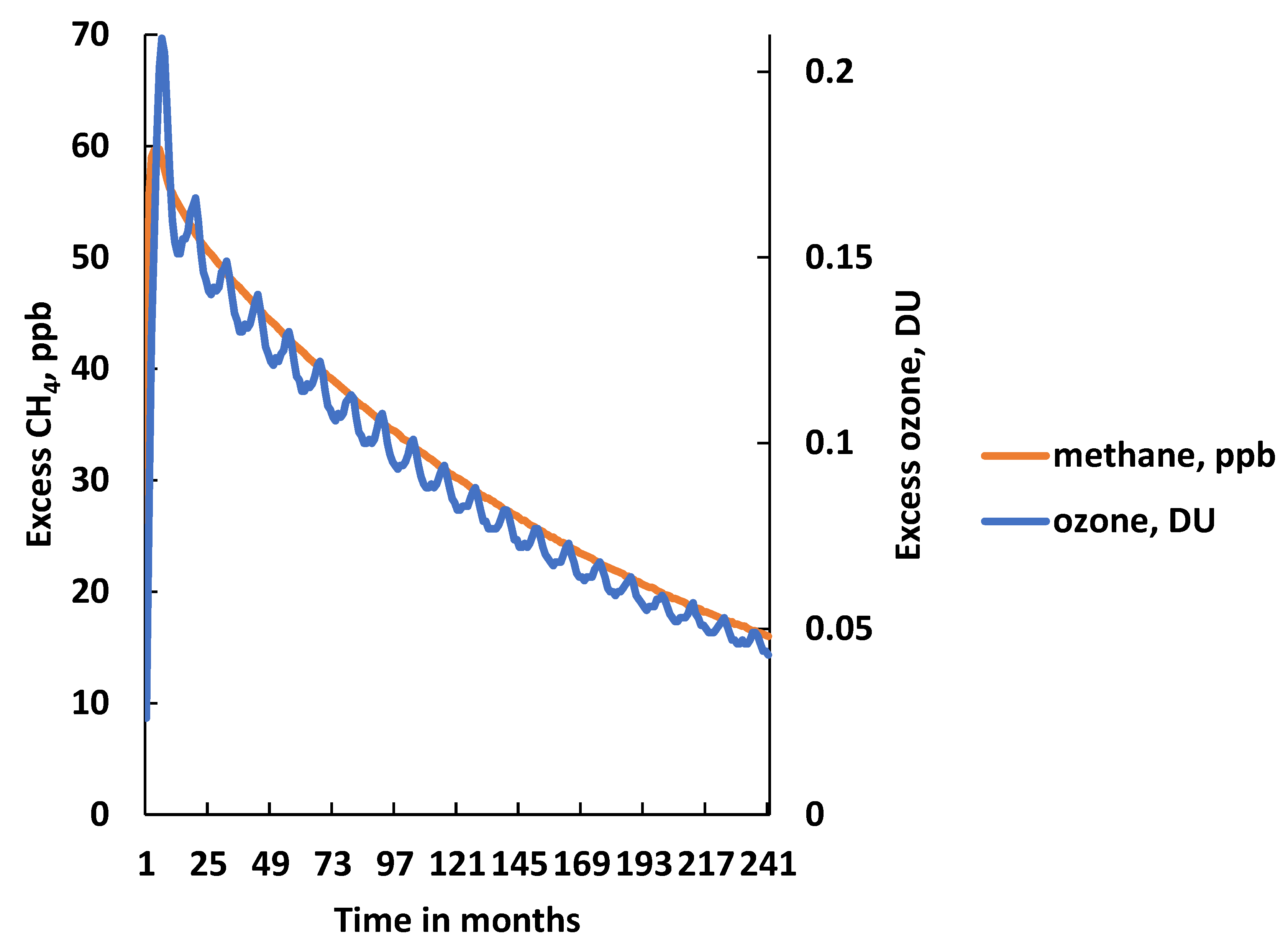
3. CH₄ Pulse Experiments under Uncertainty

TROPOS was set up with the ‘Best Estimate’ (BE) model input parameters and two model experiments were initiated. The first had the BE model inputs and the second differed from it in having an additional emission pulse of CH₄ amounting to 149 Tg. All other model inputs were identical. Both the ‘base case’ and ‘pulse case’ experiments were integrated for 20 years, with model outputs taken at the end of each month and year. The emission pulse was restricted to the latitude range from 30–56.4° N, the most important latitude range for anthropogenic emissions, and was emitted over the period 1–31 January of the first model year. This same procedure was followed with each of the many thousands of Monte Carlo replicates, with each having a ‘base case’ and a ‘pulse case’ and each a CH₄ emission pulse of 149 Tg.

At each time point, the CH₄ mixing ratios differed slightly between the pair of model experiments because of the presence of the additional CH₄ in the ‘pulse case’ experiment. Figure 1 presents the difference in the global mean CH₄ mixing ratios between the pair of ‘Best Estimate’ model experiments over the 20-year experiment. The 149 Tg emission pulse initially caused an increase in the global mean CH₄ mixing ratio of 60 ppb, as shown in Figure 1. This increase would be slightly different in each of the Monte Carlo replicates. This excess CH₄ began to decay away and this decay persisted throughout the model experiment. The decay could be accurately quantified and was found initially to be about 10% per year, dropping to about 6% per year after about 20 months. By the end of the 20-year model experiment, the excess CH₄ had decayed to 16 ppb, as shown in Figure 1. Averaged over the 3rd and subsequent years, the excess CH₄ decayed with an e-folding timescale of 15.7 years in the ‘Best Estimate’ run and 17.5 ± 9.7 years in the Monte Carlo replicates, where the quoted uncertainties are two-sigma confidence limits, here and elsewhere in this paper. This e-folding timescale is significantly longer than the atmospheric lifetime of CH₄ in the ‘base case’ experiment, which was found to be 10.9 years in the BE run (9.5 ± 5.3 in the M C replicates). The e-folding time constant corresponds to the adjustment timescale for CH₄ and is 1.45 in the BE (1.87 ± 0.6 in the MC) times longer than the atmospheric lifetime. On this basis, an FF of −0.31 (−0.45 ± 0.17 in the MC) was estimated, which partly overlapped but covered a much wider range than that reported previously [4]. The reason for the wider range is discussed later but it stems from the twenty-year model experimental time, which has allowed CH₄ to come into a steady state with each set of input data and thus extending the range of CH₄ burdens and lifetimes achieved.

The excess CH₄ decayed with an apparently longer timescale than the atmospheric lifetime because the emission pulse had caused a slight depletion in the tropospheric hydroxyl radical (OH) distribution, leading to a reduction in the OH + CH₄ reaction flux. As a result of the diminution in the CH₄ removal rate, additional CH₄ accumulated in the model troposphere. This additional CH₄ is shown as ‘new CH₄’ in blue in Figure 1. It grew steadily during the first few years, then reached a maximum after 11 years or so and then begun to decline throughout the remainder of the experiment. The ‘pulse CH₄’ decayed with the atmospheric lifetime, LT, and is shown in red in Figure 1, whereas the ‘excess CH₄’ = ‘pulse CH₄’ + ‘new CH₄’, decayed more slowly with the adjustment timescale, AT. The fraction of the ‘excess’ CH₄ that was ‘new’ was found to be 0.31 (0.45 ± 0.17).

The behaviour of CH₄ in each CH₄ ‘pulse case’ experiment was thus defined by three quantities:

• The time-integrated excess CH₄ mixing ratio in ppb years over the 20-year model experiment: 649 ppb year (668 ± 162 ppb year);
• The excess CH₄ mixing ratio at the end of the 20-year model experiment: 16 ppb (17.6 ± 11 ppb);
• The CH₄ adjustment time: 15.7 years (17.5 ± 9.7 years).

To demonstrate linearity, the ‘Best Estimate’ ‘pulse case’ experiment was repeated with emission pulses decreasing in 10% steps, down to 10% of the original 149 Tg, see

Table 2. Time-integrated radiative forcing (rf) over a 100-year time horizon for different-sized CH₄ emission pulses, together with the estimated global warming potential (GWP) with the ‘Best Estimate’ model input.

Pulse Size, Tg	Time-Integrated CH4 rf over 100 Years (mWm−2 year)	Time-Integrated O3 rf over 100 Years (mWm−2 year)	Total Time-Integrated rf over 100 Years (mWm−2 year)	Total Time-Integrated rf over 100 Years per 1 Tg Pulse (mWm−2 year) a	GWP over 100 Years Time Horizon a
149	326.7	84.7	411.4	2.761	30.1
134	293.7	76.5	370.3	2.761	30.1
119	261.1	67.6	328.7	2.757	30.1
104	228.4	59.3	287.7	2.758	30.1
89	195.7	50.9	246.7	2.759	30.1
75	163.0	42.1	205.1	2.754	30.0
60	130.3	33.7	164.1	2.753	30.0
45	97.7	25.5	123.2	2.757	30.1
30	65.0	16.6	81.6	2.739	29.9
15	32.6	8.3	40.9	2.745	29.9

Notes: ^a The number of decimal places provided does not imply numerical precision but is merely for comparison purposes.

. Time-integrated excess CH₄ mixing ratios and excess CH₄ mixing ratios at the end of the 20-year model experiments, decreased exactly in 10% steps, down to levels that were one tenth of their original values. However, the adjustment times did not change and remained exactly the same as in the original experiment. Whereas the excess CH₄ mixing ratios demonstrated accurate linearity, the CH₄ adjustment times were completely independent of pulse size.

The additional CH₄ in the ‘pulse case’ experiment also drove an increase in tropospheric O₃ production relative to the base case. This increase in O₃ production led to the build-up of an excess in tropospheric O₃ as measured as an excess in the global mean O₃ columns between the ‘pulse case’ and ‘base case’ in Dobson Units (DU). The time behaviour of excess O₃ in the ‘Best Estimate’ pulse case with 149 Tg of CH₄ is illustrated in Figure 2. The presence of a distinct seasonal cycle was evident in the excess O₃, with a summertime maximum and a wintertime minimum. This figure also presents the excess CH₄ for the same 149 Tg CH₄ pulse from Figure 1. After an initial sharp rise, excess O₃ levels decayed away with almost the same e-folding time constant as CH₄ and hence the two traces in Figure 2 almost superimposed over one another. In fact, the O₃ adjustment timescale was found to be 15.3 years, which was slightly shorter than the CH₄ adjustment time of 15.7 years in this experiment.

As with the CH₄ response, the O₃ response to the CH₄ pulse could be characterised with three quantities:

• The time-integrated excess O₃ in DU years over the 20-year model experiment: 1.85 DU year in the BE run (1.90 ± 0.75 DU year in the MC replicates);
• The excess O₃ in DU at the end of the 20-year model experiment: 0.043 DU in the BE run (0.045 ± 0.019 DU in the MC replicates);
• The O₃ adjustment time: 15.3 year in the BE run (15.7 ± 4.6 year in the MC replicates).

The time-integrated excess O₃ and the excess O₃ at the end of the 20-year model experiment were exactly linear in CH₄ pulse size in the ‘Best estimate’ experiment over the range from 149 to 14.9 Tg, see Table 2. The O₃ adjustment timescales were, however, completely independent of the CH₄ pulse size, remaining constant at 15.25 years, with deviations inside ± 1%.

4. Estimation of the Global Warming Potential for CH₄ under Uncertainty

CH₄ acts as a radiatively active trace gas by virtue of its infrared absorption spectrum. However, it also reacts in the troposphere to produce O₃, another important radiatively active trace gas, and so it is also an indirect radiatively active trace gas. In this section, an estimate is made of the global warming potential (GWP) of CH₄ based on the direct and indirect radiative forcing (rf) contributions.

The GWP of CH₄ is defined here as the ratio of the time-integrated radiative forcing resulting from the emission of 1 kg of the trace gas relative to that of 1 kg of CO₂ over a time horizon that is taken here to be 100 years [7]. That is to say:

$$\mathrm{GWP}=\frac{{{\displaystyle \int }}_0^T{\mathrm{a}}_{\mathrm{i}}{ \mathrm{c}}_{\mathrm{i}} \mathrm{dt}}{{{\displaystyle \int }}_0^T{\mathrm{a}}_{{\mathrm{CO}}_2}{ \mathrm{c}}_{{\mathrm{CO}}_2} \mathrm{dt}}$$

(2)

where a_i is the instantaneous radiative forcing due to a unit increase in the mixing ratio of trace gas, i, and c_i is the mixing ratio of the trace gas, i, remaining after time t after its release and T is the number of years over which the calculation is performed. For CH₄, the numerator has to be calculated from the sum of the impacts of CH₄ pulses on its direct radiative forcing and on its indirect radiative forcing from tropospheric O₃.

To complete the calculation of the GWP of CH₄, we use the time development of CH₄ and tropospheric O3 from each of the 5000 MC replicates, the formula for the GWP in expression (2) and the radiative efficiency parameters a_CH4 and a_O3. We took a_CH4 as 3.63 × 10⁻⁴ Wm⁻² ppb⁻¹ as the best estimate literature value from Appendix 8.A in [1], which gave a peak radiative forcing of 21.8 mWm^–2 in the ‘Best Estimate’ (BE) model experiment for a CH₄ emission pulse of 149 Tg. The time-integrated CH₄ radiative forcing in the 20-year model experiment was found to be 235 mWm⁻² year in the BE run (242 ± 59 mWm⁻² year in the MC replicates). To complete the GWP calculation, the time-integrated CH₄ radiative forcing is required over the complete 100-year time horizon so the plot in Figure 1 needed extending over the remaining 80 years. This time extension was not possible with TROPOS because of the long run times involved. However, the CH₄ response could be extended to the end of the time horizon using the concept of trace gas adjustment timescales. That is to say, it was assumed that the excess CH₄ continued to decay exponentially with the CH₄ adjustment timescale throughout year 21 and subsequently through to the end of year 99. Both the excess CH₄ at the end of the 20-year model experiment, hence its radiative forcing, and the CH₄ adjustment time were well defined quantities. The time extension added a further time-integrated excess CH₄ of 250 ppb year in the BE run (333 ± 376 ppb year in the MC replicates) and 90.9 mWm⁻² year in the BE run (121 ± 136 mWm⁻² year in the MC replicates) of radiative forcing for a 149 Tg CH₄ pulse. Altogether, the time-integrated radiative forcing from CH₄ over the entire 100-year time horizon amounted to 327 mWm⁻² year in the BE run (363 ± 195 mWm⁻² year in the MC replicates).

The estimation of the radiative forcing consequences of changes in the tropospheric distribution of O₃ is not straightforward [29]. A description of a methodology is available that starts by characterising O₃ column amounts on a 5° latitude × 5° longitude grid in Dobson Units (DU) and uses a complex radiation code to relate these column amounts to radiative forcing [29]. Using this approach [29], gridded estimates of radiative forcing per DU were employed to estimate the radiative forcing consequences of the changes in tropospheric O₃ column amounts resulting from the CH₄ emission pulses. In response to a 149 Tg CH₄ emission pulse, the excess O₃ response increased to a maximum of 0.21 DU in the ‘Best Estimate’ model experiment before decaying away with the O₃ adjustment timescale. The time-integrated excess O₃ over the 20-year model experiment amounted to 1.85 DU year in the BE run (1.90 ± 0.75 DU year in the MC replicates) or 62.5 mWm⁻² year in the BE (64 ± 25 mWm⁻² year in the MC replicates). Extension to the 100-year time horizon using the O₃ adjustment timescale amounted to an additional 22.2 mWm⁻² year in the BE run (24.0 ± 14 mWm⁻² year in the MC replicates). The total radiative forcing from the excess O₃ was therefore 84.7 mWm⁻² year in the BE run (88.2 ± 34 mWm⁻² year in the MC replicates) for a 149 Tg CH₄ emission pulse.

To calculate the CH₄ GWP, the numerator of expression (2) was formed by adding together the CH₄ and tropospheric O₃ forcing terms to make 411 mWm⁻² year in the ‘Best Estimate’ model experiment, see Table 2, and 451 ± 190 mWm⁻² year in the Monte Carlo replicates. Dividing this total radiative forcing by the pulse size of 149 Tg and dividing by the denominator of Equation (2), which was taken to be 0.0917 mWm⁻² year from Appendix A.8 in [1], gave 30.1 in the BE run (33 ± 14 in the MC replicates) over a 100-year time horizon for 1 Tg emission pulses.

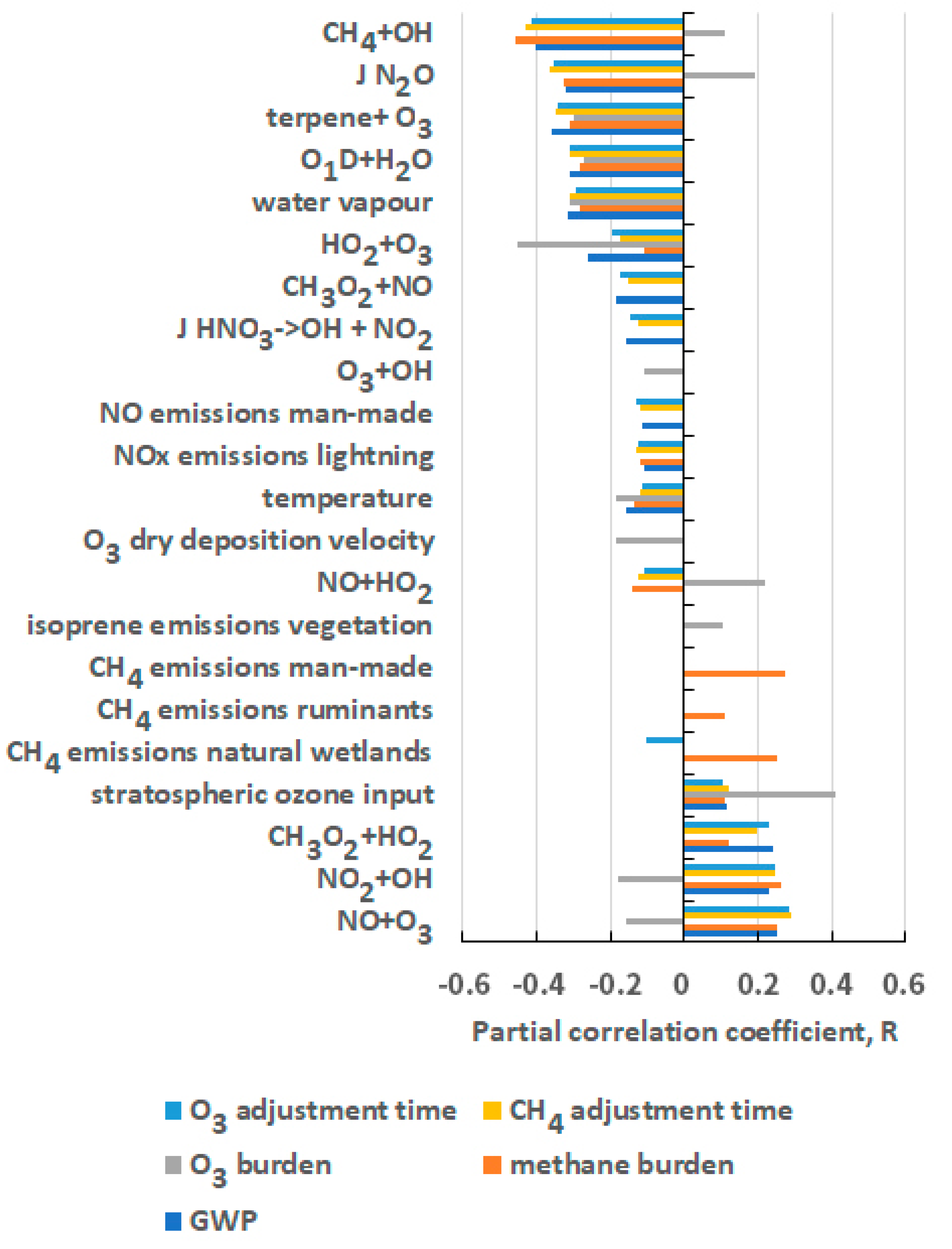
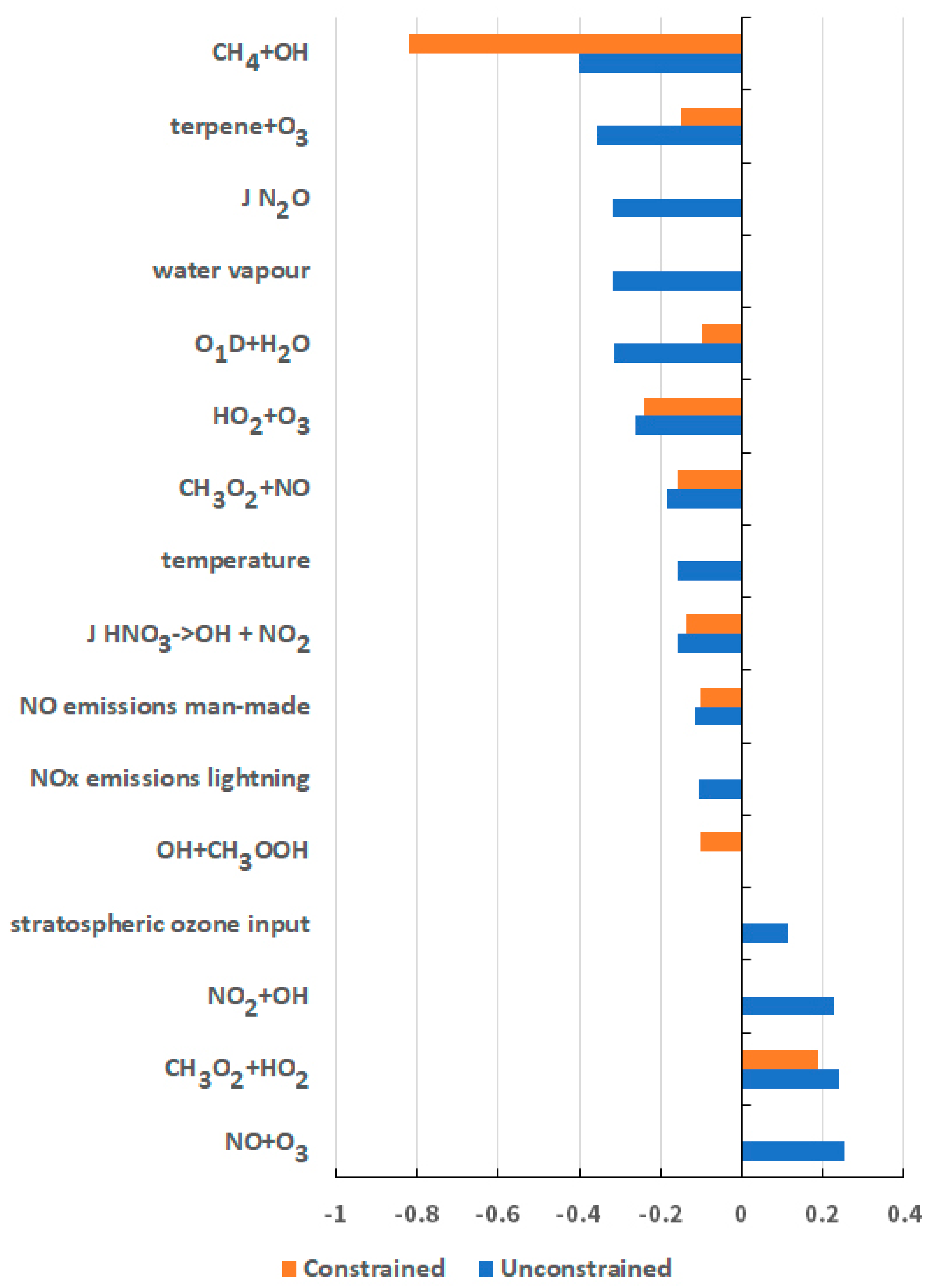
5. Origins of the Uncertainty in the GWP for CH₄

Having quantified the GWP for CH₄ and its 2-sigma confidence limits, the next step is to ascertain which are the most important input uncertainties that drive the uncertainties in the GWP. In Figure 3, the partial correlation coefficients are presented for those parameters that gave R values in the range −0.1 > R > +0.1. Also shown are analogous plots for additional outputs that influenced strongly the estimated GWPs, including the burdens of CH4 and O₃ and the adjustment timescales for CH₄ and O₃. Altogether 22 input parameters contributed most to output uncertainty and these comprised 12 chemical kinetic rate coefficients, six emission sources and four meteorological and physical input parameters. These most important parameters are listed in

Table 3. Details of the most important input parameters contributing to the uncertainty in the burdens of O₃ and CH₄, the adjustment times for CH₄ and O₃ and the GWP for CH₄.

Chemical Kinetic Rate Coefficients	Emission Sources and Sectors
CH4 + OH	NOx from man-made sources
O1D + H2O	NOx from lightning
HO2 + O3	CH4 from man-made sources
O3 + OH	CH4 from natural wetlands
NO + HO2	CH4 from ruminants
NO2 + OH	isoprene from vegetation
NO + O3	-
CH3O2 + HO2	-
Chemical Kinetic Rate Coefficients	Meteorological and Physical Parameters
CH3O2 + NO	Water vapour
terpene + O3	Temperature
J HNO3	O3 deposition velocity
J N2O	O3 input from stratosphere

.

The twelve most important chemical kinetic rate coefficients include several chemical processes that play a crucial role in establishing the fast, photochemical balance of the troposphere. These processes include CH₄ + OH, O¹D + H₂O, HO₂ + O₃, CH₃O₂ + NO, O₃ + OH, HO₂ + O₃, NO + HO₂, NO₂ + OH and CH₃O₂ + HO₂. In addition, the NO + O₃ reaction controls the ratio of NO to NO₂, which in turn controls the relative rates of HO₂ to OH recycling versus the loss of OH. The terpene + O₃ reaction, together with the O₃ deposition velocity, controls the lifetime of O₃ close to the surface over forested areas. Two photolysis processes are listed in Table 3: the photolysis rate coefficient (J) for nitric acid and that for N₂O in the stratosphere. The former controls the long-range transport of nitric acid and its renoxification back to NO_x and the former controls the altitude profile of NO_x in the lower stratosphere, the NO_x-catalysed destruction of O₃ there and hence the stratosphere–troposphere exchange flux of O₃ into the troposphere.

Of all of the twelve chemical processes in Figure 3 and Table 3, the OH + CH₄ reaction clearly dominates as a source of uncertainty in the CH₄ GWP and its drivers. An important contribution to the overall uncertainty in this rate coefficient comes from the uncertainty in its temperature coefficient, which is one of the largest of all the processes in the fast, photochemical balance of the troposphere.

The six emission sources and sectors listed in Table 3 involve three trace gases: NO_x, CH4 and isoprene. Emissions of NO_x and CH₄ provide important drivers of the fast photochemistry of the troposphere through the formation of CH₄ oxidation products (CO, formaldehyde and methyl peroxy radicals) and the control they influence on the tropospheric distribution of CH₄. Isoprene emissions from vegetation act as an important source of CO, HO₂ and formaldehyde.

Uncertainty due to meteorological and physical parameters is strongly influenced by the uncertainties due to water vapour and temperature biases and to the parameters that control stratosphere–troposphere exchange and the deposition of O₃, as shown in Table 3.

6. Discussion and Conclusions

In Section 2.2, above, it was noted that the atmospheric lifetime of CH₄ from the 5000 MC replicates (9.5 ± 5.4 years) had a two-sigma confidence range that was significantly wider than that reported in the observations [23] (11.2 ± 1.3 years). That is to say, the two-sigma confidence range of the MC replicates was over four-fold wider than that in the observations. It was concluded that the two-sigma confidence range in the MC analysis was unrealistically wide and hence some of the 5000 input parameter combinations in the MC analysis may have been unrealistic. Further work is planned to investigate the reasons why some input parameter combinations appeared unrealistic and whether it would be possible to reduce their assumed uncertainty ranges accordingly.

If the MC analysis was constrained by the observed atmospheric lifetime for CH₄, then 1249 MC replicates (about one quarter of the total) would be retained and 3751 (about three quarters of the total) would be rejected. The GWP for CH₄ calculated with only the retained replicates would then be 37 ± 10, compared with 33 ± 14 based on all 5000 MC replicates. The rejection of the replicates with infeasible CH₄ lifetimes caused a 12% or so increase in the GWP and a somewhat larger 30% decrease in the 95% confidence interval. This value of 37 ± 10 is outside the range of 28–34 given by Table 8.7 in [1], where the range addresses the issue of the non-inclusion (28) or inclusion (34) of climate-carbon feedbacks. For the purposes of this comparison, we take the non-inclusion value and conclude that our value obtained with the feasible MC input data overestimates the IPCC literature value [1] by about 24% and is considerably higher than our previously reported 23.2 [17] from nearly 20 years ago.

The atmospheric lifetime constraint was then used to adjust the weightings of the replicates in the multiple linear regression analysis of the uncertainties in the CH₄ GWP. Those MC replicates that gave plausible CH₄ lifetimes in their base runs were given a weighting of unity and those that did not were given a weighting factor that was several orders of magnitude smaller. With the constraint applied and the weightings adjusted, the partial correlation coefficients for the 183 input parameters shifted significantly relative to those without the constraint, see Figure 4. A significant increase was found in the partial correlation coefficient due to the CH₄ + OH rate coefficient. With the constraint applied, the fraction of the uncertainty in the GWP for CH₄ due to the CH₄ + OH rate coefficient increased from 16% to 67%. There was a compensating decrease in the fraction of the uncertainty due to the rate coefficients for terpene + O₃, O¹D + H₂O, NO₂ + OH and the NO + O₃ reactions. Uncertainties due to the photolysis rate of N₂O in the stratosphere, temperature and water vapour biases and stratospheric O₃ input also reduced dramatically. Overall uncertainty was reduced significantly by the application of the CH₄ lifetime constraint and the only significant contributions remaining were from the CH₄ + OH, CH₃O₂ + HO₂, CH₃O₂ + NO and the terpene + O₃ rate coefficients, see Figure 4.

Our recommendation for the CH₄ GWP is therefore 37 ± 10 over a 100-year time horizon and means that the time-integrated radiative forcing from the release of 1 Tg of CH₄ over a 100-year time horizon is equivalent to that from 37 ± 10 Tg of CO₂. We also conclude that the principal area of uncertainty in this recommended GWP arises in the chemical kinetic rate coefficient input data for the five highlighted chemical processes. Additional research efforts focused on reducing the uncertainties in these rate coefficients may potentially reduce the uncertainties in the estimated CH₄ GWP.

References

1. IPCC. Climate Change 2018: The Physical Science Basis; Cambridge University Press: Cambridge, UK, 2018. [Google Scholar]
2. United Nations Framework Convention on Climate Change. United Nations Framework Convention on Climate Change; UNFCCC: New York, NY, USA, 1992. [Google Scholar]
3. Etheridge, D.M.; Pearman, G.I.; Fraser, P.J. Changes in tropospheric methane between 1841 and 1978 from a high accumulation-rate Antarctic ice core. Tellus B 1992, 44, 282–294. [Google Scholar] [CrossRef]
4. IPCC. Climate Change 1994. In Intergovernmental Panel on Climate Change; Cambridge University Press: Cambridge, UK, 1995. [Google Scholar]
5. Turner, A.J.; Frankenburg, C.; Wennberg, P.O.; Jacob, D.J. Ambiguity in the causes for decadal trends in atmospheric methane and hydroxyl. Proc. Natl. Acad. Sci. USA 2017, 114, 5367–5372. [Google Scholar] [CrossRef] [PubMed] [Green Version]
6. Rigby, M.; Montzka, S.A.; Prinn, R.G.; White, J.W.; Young, D.; O’Doherty, S.; Lunt, M.F.; Ganesan, A.L.; Manning, A.J.; Simmonds, P.G.; et al. Role of atmospheric oxidation in recent methane growth. Proc. Natl. Acad. Sci. USA 2017, 114, 5373–5377. [Google Scholar] [CrossRef] [PubMed] [Green Version]
7. IPCC. Climate Change: The IPCC Scientific Assessment; Cambridge University Press: Cambridge, UK, 1990. [Google Scholar]
8. Shine, K.P. The global warming potential—The need for an interdisciplinary retrial. Clim. Chang. 2009, 96, 467–472. [Google Scholar] [CrossRef] [Green Version]
9. Shine, K.P.; Fuglestvedt, J.S.; Hailemariam, K.; Stuber, N. Alternatives to the global warming potential for comparing climate impacts of emissions of greenhouse gases. Clim. Chang. 2005, 68, 281–302. [Google Scholar] [CrossRef] [Green Version]
10. Derwent, R.G.; Parrish, D.D.; Galbally, I.E.; Stevenson, D.S.; Doherty, R.M.; Naik, V.; Young, P.J. Uncertainties in models of tropospheric ozone based on Monte Carlo analysis: Tropospheric ozone burdens, atmospheric lifetimes and surface distributions. Atmos. Environ. 2018, 180, 93–102. [Google Scholar] [CrossRef] [Green Version]
11. Derwent, R.G. Monte Carlo analyses of the uncertainties in the predictions from global tropospheric ozone models: Tropospheric burdens and seasonal cycles. Atmos. Environ. 2020, 213, 117545. [Google Scholar] [CrossRef]
12. Bolin, B.; Rodhe, H. Note on concepts of age and transit-time in natural reservoirs. Tellus 1973, 25, 58–62. [Google Scholar] [CrossRef]
13. Prather, M.J. Lifetimes and eigenstates in atmospheric chemistry. Geophys. Res. Lett. 1994, 21, 801–804. [Google Scholar] [CrossRef] [Green Version]
14. Isaksen, I.S.A.; Hov, O. Calculation of trends in tropospheric O3, OH, CH4 and NOx. Tellus B 1987, 39, 271–285. [Google Scholar] [CrossRef] [Green Version]
15. Prather, M.J. Lifetimes and time scales in atmospheric chemistry. Phil. Trans. R. Soc. A 2007, 365, 1705–1726. [Google Scholar] [CrossRef] [PubMed]
16. Wild, O.; Prather, M.J. Excitation of the primary tropospheric chemical mode in a global three-dimensional model. J. Geophys. Res. 2000, 105, 24647–24660. [Google Scholar] [CrossRef] [Green Version]
17. Derwent, R.G.; Collins, W.J.; Johnson, C.E.; Stevenson, D.S. Transient behaviour of tropospheric ozone precursors in a global 3-D CTM and their indirect greenhouse effects. Clim. Chang. 2001, 49, 463–487. [Google Scholar] [CrossRef]
18. Hough, A.M.; Derwent, R.G. Changes in the global concentration of tropospheric ozone due to human activities. Nature 1990, 344, 645–648. [Google Scholar] [CrossRef]
19. Utembe, S.R.; Watson, L.A.; Shallcross, D.E.; Jenkin, M.E. A Common Representative Intermediates (CRI) mechanism for VOC degradation. Part 3: Development of a secondary organic aerosol module. Atmos. Environ. 2009, 43, 1982–1990. [Google Scholar] [CrossRef]
20. Utembe, S.R.; Cooke, M.C.; Archibald, A.T.; Shallcross, D.E.; Derwent, R.G.; Jenkin, M.E. Simulating secondary organic aerosol in a 3-D Lagrangian chemistry transport model using the reduced Common Representative Intermediates mechanism (CRI v2-R5). Atmos. Environ. 2011, 45, 1604–1614. [Google Scholar] [CrossRef]
21. Curtis, A.R.; Sweetenham, W.P. FACSIMILE Release H User’s Manual; AERE Report R11771; H.M. Stationery Office: London, UK, 1987. [Google Scholar]
22. Cooper, O.R.; Parrish, D.D.; Ziemke, J.; Balashov, N.V.; Cupeiro, M.; Galbally, I.E.; Gilge, S.; Horowitz, L.; Jensen, N.R.; Lamarque, J.-F.; et al. Global distribution and trends of tropospheric ozone: An observation-based review. Elem. Sci. Anthr. 2014, 2, 000029. [Google Scholar] [CrossRef]
23. Naik, V.; Voulgarakis, A.; Fiore, A.M.; Horowitz, L.W.; Lamarque, J.F.; Lin, M.; Prather, M.J.; Young, P.J.; Bergmann, D.; Cameron-Smith, P.J.; et al. Pre-industrial to present-day changes in tropospheric hydroxyl and methane lifetime from the Atmospheric Chemistry and Climate Model Intercomparison Project (ACCMIP). Atmos. Chem. Phys. 2013, 13, 5277–5298. [Google Scholar] [CrossRef] [Green Version]
24. Young, P.J.; Archibald, A.T.; Bowman, K.W.; Lamarque, J.F.; Naik, V.; Stevenson, D.S.; Tilmes, S.; Voulgarakis, A.; Wild, O.; Bergmann, D.; et al. Pre-industrial to end 21st century projections of tropospheric ozone from the Atmospheric Chemistry and Climate Model Intercomparison Project. Atmos. Chem. Phys. 2013, 13, 2063–2090. [Google Scholar] [CrossRef] [Green Version]
25. Ziemke, J.R.; Chandra, S.; Labow, G.J.; Bhartia, P.K.; Froidevaux, L.; Witte, J.C. A global climatology of tropospheric and stratospheric ozone derived from Aura OMI and MLS measurements. Atmos. Chem. Phys. 2011, 11, 9237–9251. [Google Scholar] [CrossRef] [Green Version]
26. Revell, L.E.; Stenke, A.; Tummon, F.; Feinberg, A.; Rozanov, E.; Peter, T.; Abraham, N.L.; Akiyoshi, H.; Archibald, A.T.; Butchart, N.; et al. Tropospheric ozone in CCMI models and Gaussian process emulation to understand biases in the SOCLv3 chemistry-climate model. Atmos. Chem. Phys. 2018, 18, 16155–16172. [Google Scholar] [CrossRef] [Green Version]
27. Newsome, B.; Evans, M. Impact of uncertainties in inorganic chemical rate constants on tropospheric composition and ozone radiative forcing. Atmos. Chem. Phys. 2017, 17, 14333–14352. [Google Scholar] [CrossRef] [Green Version]
28. Wild, O.; Voulgarakis, A.; O’Connor, F.; Lamarque, J.F.; Ryan, E.; Lee, L. Global sensitivity analysis of chemistry-climate model budgets of tropospheric ozone and OH: Exploring model diversity. Atmos. Chem. Phys. 2020. [Google Scholar] [CrossRef] [Green Version]
29. Stevenson, D.S.; Young, P.J.; Naik, V.; Lamarque, J.F.; Shindell, D.T.; Voulgarakis, A.; Skeie, R.B.; Dalsoren, S.B.; Myhre, G.; Berntsen, T.K.; et al. Tropospheric ozone changes, radiative forcing and attribution to emissions in the Atmospheric Chemistry and Climate Model Intercomparison Project (ACCMIP). Atmos. Chem. Phys. 2013, 13, 3063–3085. [Google Scholar] [CrossRef] [Green Version]
Figure 1. Time development of the excess global mean CH4 mixing ratio following the addition of a 149 Tg CH4 emission pulse, showing the ‘excess’ CH4 = ‘pulse’ CH4 + ‘new’ CH4 as the upper curve, the pulse CH4 (red area) and new CH4 (blue area), based on a similar figure taken from ref. [13].
Atmosphere 11 00486 g001
Figure 2. Time development of the excess global mean CH4 mixing ratio and the excess global mean O3 column in Dobson Units following the addition of a 149 Tg CH4 emission pulse.
Atmosphere 11 00486 g002
Figure 3. Partial correlation coefficients from the multiple linear regression analyses of the adjustment times, burdens and the resulting GWP for CH4 on the 183 uncertain model input parameters.
Atmosphere 11 00486 g003
Figure 4. Partial correlation coefficients from the multiple linear regression analyses of the GWP for CH4 on the 183 uncertain model input parameters in the unconstrained Monte Carlo replicates (blue bars) and those with CH4 lifetimes constrained in the range 11.2 ± 1.3 years (red bars).
Atmosphere 11 00486 g004