The Microphysical Properties of a Sea-Fog Event along the West Coast of the Yellow Sea in Spring

Abstract

The microphysics and visibility of a sea-fog event were measured at the Qingdao Meteorological Station (QDMS) (120°19′ E, 36°04′ N) from 5 April to 8 April 2017. The two foggy periods with low visibility (<200 m) lasted 31 h together. The mean value of the average liquid water content (LWC) was 0.057 g m⁻³, and the mean value of the number concentration (NUM) was 64.4 cm⁻³. We found that although large droplets only constituted a small portion of the total number of the concentration; they contributed the majority of the LWC and therefore determined ~76% of total extinction of the visibility. The observed droplet-size distribution (DSD) exhibited a new bimodal Gaussian (G-exponential) distribution function, rather than the well-accepted Gamma distribution. This work suggests a new distribution function to describe fog DSD, which may help to improve the microphysical parameterization for the Yellow Sea fog numerical forecasting.

1. Introduction

Sea fog is a fog that occurs under oceanic conditions, which may severely influence marine navigation, low-level flight conditions, and land transportation [1,2,3,4]. To reduce loss of life and property, fog forecasting is important. Meanwhile, parameterization of complicated microphysical processes is essential to numerical models for fog forecasting [5,6].

Microphysical parameters, such as liquid water content (LWC), number concentration (NUM), and droplet-size distribution (DSD), have a significant influence on fog formation, development, and dissipation, which eventually affect visibility [7,8,9,10]. DSD affects the fog-settling rate and the lifetime of a fog layer [6,11]. DSD is important in the study of atmospheric radiation and for the parameterization of the rain and cloud microphysical processes used in forecasting models [12,13]. Fog-microphysics studies can not only help understand fog microphysical processes but also help improve fog numerical forecasting [3].

A great effort has been devoted to finding an appropriate analytical expression for describing DSD. The Gamma function has been commonly used for describing land-fog DSD [14,15]. Niu et al. (2009) [14] showed that the observed fog DSD in Nanjing, China can be well-described by the Gamma distribution. Schmitt et al. (2013) [15] characterized the DSD of ice fog in Interior Alaska using the Gamma distribution. However, it is not clear whether the Gamma distribution may also be applicable to sea fogs or fogs near the coastline [4].

The Yellow Sea is the foggiest area in China’s adjacent seas. The Qingdao Meteorological Station (QDMS, shown in Figure 1), next to the Yellow Sea, records more than 50 foggy days annually [16]. (A foggy day is defined as being at least one record of fog on that day.) To enhance the understanding of sea-fog microphysics in the Yellow Sea, an in situ campaign was carried out at QDMS in spring from 5 April to 8 April, 2017. The rest of the paper is organized as follows: Section 2 introduces the experiment site, the instruments used for data collection, and the calculations of the fog properties. Section 3 presents and discusses the results, including the general characteristics of microphysics and fog DSD. Finally, a new scheme based on a Gaussian (G-exponential) distribution function is suggested for calculating visibility. Concluding remarks are presented in Section 4.

2. Data and Methodology

2.1. Observation

The QDMS is located in Shandong Province, China (120°19′ E, 36°04′ N), 76 m above sea level, and about 1.5 km from the Yellow Sea (Figure 1). It is one of the National Ordinary Stations belonging to the China Meteorological Administration.

The microphysical properties of the sea fog, such as LWC, NUM, and DSD, were measured by an FM-120 fog monitor, which provided fog droplet diameters from 2 to 50 μm, with a 1-μm resolution from 2 to 14 μm, and with a 2-μm resolution from 14 to 50 μm. The sampling frequency range was 1 Hz in this observation.

Visibility was automatically measured by a visibility meter (FD12) at the same site, which evaluated the meteorological optical range (MOR) by measuring the scattering of infrared light. The measurement range was 10 to 50,000 m, and the sampling time interval was set to 10 min. An automatic meteorological station recorded air temperature, relative humidity (RH), and surface wind every 10 minutes. We employed buoy data at Changmenyan station (CMY) off the Qingdao coast (Figure 1). The buoy recorded visibility, sea-air temperature (SAT), sea-surface temperature (SST), and sea-surface wind every hour.

2.2. Calculation Methods

The NUM (cm⁻³) and LWC (g m⁻³) of the whole spectra can be calculated as follows [14]:

$$\mathrm{NUM}=\sum \mathrm{n}\left(\mathrm{r}\right), \left(\mathrm{r}=1.25,1.75,\dots ,6.75,7.5,\dots ,24.5\right),$$

(1)

$$\mathrm{LWC}=\sum 1\times {10}^{-6}\times \mathsf{\rho }\times \frac{4\mathsf{\pi }}{3}{\mathrm{r}}^3\mathrm{n}\left(\mathrm{r}\right), \left(\mathrm{r}=1.25,1.75,\dots ,6.75,7.5,\dots ,24.5\right),$$

(2)

where r is the mean radius (in the unit of μm) with interval 0.5 μm from 1.25 to 6.75 μm and 1 μm from 7.5 to 24.5 μm, ρ = 10⁻⁶ g m⁻³ is the density of water, and $\mathrm{l}\left(\mathrm{r}\right)=1\times {10}^{-6}\times \mathsf{\rho }\times \frac{4\pi }{3}{\mathrm{r}}^3\mathrm{n}\left(\mathrm{r}\right)$ is the liquid water content for different r.

In general, the k-order radius moment (${\mathrm{m}}_{\mathrm{k}}$) can be calculated with the following expression [14]:

$${\mathrm{m}}_{\mathrm{k}}=\sum {\mathrm{r}}^{\mathrm{k}}\frac{\mathrm{n}\left(\mathrm{r}\right)}{\mathrm{NUM}} \left(\mathrm{k}=1,2,\cdots \right),$$

(3)

and the mean radius can be calculated as $\overline{\mathrm{r}}={\mathrm{m}}_1$.

The total sum of squares (sst) is defined as the sum of the squared differences of each observation from the overall mean [17]:

$$\mathrm{sst}={\sum }_{\mathrm{i}=1}^{\mathrm{N}}{({\mathrm{y}}_{\mathrm{i}}-\overline{\mathrm{y}})}^2,$$

(4)

where $\overline{\mathrm{y}}$ is the mean of observation and ${\mathrm{y}}_{\mathrm{i}}$ is $y$ value for observation $\mathrm{i}$. The decrease of sst indicates that the observation value tends to average.

The sum of squared errors ($\mathrm{sse}$) is the sum of the squares of residuals [18]. It is a measure of the discrepancy between the observed data and an estimation model:

$$\mathrm{sse}={\sum }_{\mathrm{i}=1}^{\mathrm{N}}{({\mathrm{y}}_{\mathrm{i}}-\widehat{{\mathrm{y}}_{\mathrm{i}}})}^2,$$

(5)

where $\widehat{{\mathrm{y}}_{\mathrm{i}}}$ is the value of the variable to be estimated. The decrease of sse indicates a better extent to which the dependent variable is estimable.

The coefficient of determination (R²) is interpreted as the proportion of the variance in the dependent variable that is estimable from the independent variable [18]

$${\mathrm{R}}^2=\frac{\mathrm{sst}-\mathrm{sse}}{\mathrm{sst}}=1-\frac{\mathrm{sse}}{\mathrm{sst}},$$

(6)

R² ranges from 0 to 1. The closer R² is to 1, the better extent to which the dependent variable is estimable.

3. Results

3.1. General Characteristics

Figure 2 highlights, in the white background, the periods with visibility lower than 1000 m at QDMS and CMY and temporal evolution of SST, SAT, RH, and surface wind from 6 April to 8 April 2017. These periods are common to both QDMS and CMY, due to their close proximity. In addition, the visibility trends at the two stations are very similar, but most of the sea fog times the visibility observed at CMY are lower than that at QDMS, which reveals that the fog at sea is stronger than that on land. Moreover, the timing of the fog occurrence at the two stations differs. Compared with QDMS, the visibility measured at the CMY decreased below 1000 m 1 h earlier, and increased above 1000 m 2 h later, indicating that the sea fog first arrived at the coastal sea and then marched into land in the morning. A previous study shows that about 80–90% of the fog over the Yellow Sea in this season is advection fog [1]. Later in the midday, as temperature increased, the air became unsaturated because of the decrease in the relative humidity, and the sea fog over land dissipated more quickly than over the sea, as indicated by the increase of visibility. At the beginning of advection-fog formation, the sea-surface air temperature (SAT) is greater than the sea-surface temperature (SST) when the warm air moves over the cold-sea surface. After the advection fog is developed, the fog’s top layer cools radiatively. Together with the action of turbulent mixing, the temperature of the fog layer may decrease below SST. Yang et al. (2018) found that 33% of advection fog in the western Yellow Sea has a temperature below SST [19].

The fog event began at around 0827 UTC 6 April 2017, and dissipated at 0230 UTC 8 April 2017 (LST = UTC + 8 h). From 0930 UTC 6 April to 0040 UTC 7 April, and from 1000 UTC 7 April to 0110 UTC 8 April, the visibility remained below 200 m. The two fog periods lasted 31 h. Visibility rose above 1000 m due to the increase in temperature and decrease in relative humidity from 0349 UTC 7 April to 0908 UTC 7 April. The major microphysics properties during the fog events are summarized in

Table 1. Means values of key microphysical properties during the two foggy periods.

	Microphysical Properties
	Liquid Water Content (g m−3)	Number Concentration (cm−3)	Mean Radius (μm)	Peak Radius (μm)
Maximum	0.172	146.9	6.7	3.3
Minimum	0.001	1.0	1.9	1.8
Average	0.057	64.4	4.0	2.7

. The mean value of the LWC was 0.057 g m⁻³, the mean value of the radius was 4.0 μm, and the mean value of the NUM was 64.4 cm⁻³ during these two fog events. The mean value of LWC is comparable with that observed (0.041 g m⁻³) in Tianjin [20], but the mean value of NUM is only 10.8% with that observed (596 cm⁻³) in Tianjin. With a lot of condensation nuclei in an industrial city (Tianjin), water vapor condenses on condensation nuclei, producing a large number of small droplets [1].

3.2. Fog Droplets Microphysical Characteristics

The number density distribution, n(r) in Equation (1), measured over QDMS during the two fog periods is averaged. We divide n(r) by NUM to obtain the relative NUM density distribution (Figure 3, red). We also calculate l(r) using Equation (2), which is then divided by LWC to obtain the relative LWC density distribution (Figure 3, blue). Both distributions exhibit a bimodal structure, but the locations of the primary peaks are different: n(r) shows a primary maximum (~23%) at 2.75 μm and a secondary peak (~3%) at 8.5 μm. On the contrary, because of the factor r³ in Equation (2), the secondary peak in n(r) becomes the primary peak in l(r): l(r) shows a primary maximum (~23%) at 12.5 μm and a secondary peak (~7%) at 3.25 μm. Based on these distributions, we define an empirical threshold at a radius equal to 5 μm, below which the droplets are defined as “small”; otherwise, the droplets are defined as “large”. Figure 3 shows that small droplets constitute the majority of the total NUM, but it is the large droplets that constitute the majority of the total LWC.

The partitioning of small and large droplets is time independent: we calculate the NUM of the small (red) and large (grey) droplets at each 1-minute observational interval and plot then against the total NUM at the same 1-minute interval (Figure 4a). The regression line for small droplets is given by $\mathrm{y}=0.85\mathrm{X}-1.77$, with R² equal to 0.98. The regression line for large droplets is given by $\mathrm{y}=0.15\mathrm{X}+1.77$, with R² equal to 0.62. Thus, ~85% of the droplets are small, regardless of the total NUM and the time of the measurement.

We also calculate the 1-minute-average LWC of small and large droplets (Figure 4b). The regression line for small droplets is $\mathrm{y}=0.07\mathrm{X}+0.00195,$ with R² equal to 0.5006. The regression line for large droplets is $\mathrm{y}=0.93\mathrm{X}-0.00195,$ with R² equal to 0.9947. Thus, 93% of the total LWC is decided by the large droplets, also regardless of the total NUM and the time of measurement.

Using visibility as the criterion, the fogging process can be divided into three stages: the formation stage (when the visibility drops from 1000 m to its lowest level), the development stage (after the visibility drops to its lowest level and remains basically constant for more than 30 min), and the dissipation stage (when the visibility increases noticeably from the lowest value to 1000 m) [20]. Figure 5 shows the size distribution characteristics of fog droplets at each stage during the two fog periods. During the formation stage, the droplet-size spectrum was narrow, and the droplet diameter was small. During the development stage, the number of all sizes of fog droplets increased, and the droplet-size spectrum became wide. During the dissipation stage, the number of all sizes of fog droplets decreased, especially the large fog droplets.

3.3. Analytical Expression for Fog DSD

The Gamma function has been commonly used for describing DSD [14,15,21]. Whether the DSD of sea fog can be described well by the Gamma distribution is examined, as follows:

$$\mathrm{n}\left(\mathrm{r}\right)={\mathrm{N}}_0{\mathrm{r}}^{\mathsf{\mu }}{\mathrm{e}}^{-\mathsf{\lambda }\mathrm{r}},$$

(7)

where $\mathrm{r}$ and $\mathrm{n}\left(\mathrm{r}\right)$ are droplet radii and the number of droplets, respectively, and ${\mathrm{N}}_0$, $\mathsf{\lambda }$, and $\mathsf{\mu }$ are the intercept, slope, and shape parameters, respectively [14].

Based on Equation (7), Liu (1992, 1993) [8,22] proposed a simple statistical method to identify the statistical distribution pattern, which was used to investigate if the statistical pattern of the fog DSD follows the Gamma distribution, skewness (${\mathrm{S}}_{\mathrm{k}}$) and kurtosis (${\mathrm{K}}_{\mathrm{u}}$) are defined as:

$${\mathrm{S}}_{\mathrm{k}}=\frac{{\mathrm{m}}_3-3{\mathrm{m}}_1{\mathrm{m}}_2+2{\mathrm{m}}_1^3}{{\left({\mathrm{m}}_2-{\mathrm{m}}_1^2\right)}^{3/2}},$$

(8)

$${\mathrm{K}}_{\mathrm{u}}=\frac{{\mathrm{m}}_4-4{\mathrm{m}}_1{\mathrm{m}}_3+6{\mathrm{m}}_1^2{\mathrm{m}}_2-3{\mathrm{m}}_1^4}{{\left({\mathrm{m}}_2-{\mathrm{m}}_1^2\right)}^2}-3,$$

(9)

where m₁, m₂, m₃, and m₄ are 1-order, 2-order, 3-order, and 4-order radii moments, respectively.

Given the ${\mathrm{S}}_{\mathrm{k}}$ and ${\mathrm{K}}_{\mathrm{u}}$, the skewness and kurtosis deviation coefficients (${\mathrm{C}}_{\mathrm{s}}$ and ${\mathrm{C}}_{\mathrm{k}}$) can be calculated for the Gamma distribution as follows:

$${\mathrm{C}}_{\mathrm{s}}=\frac{{\mathrm{S}}_{\mathrm{k}}^2}{4}=\frac{1}{1+\mathsf{\mu }}=\frac{{\mathrm{K}}_{\mathrm{u}}}{6}={\mathrm{C}}_{\mathrm{k}},$$

(10)

Figure 6 shows that most of the dots clearly deviate from the diagonally straight line, indicating that the Yellow Sea fog DSD is different from DSD in some land fogs [14] that are described well by the Gamma distribution with a varying μ that satisfies the diagonally straight line.

In order to describe the bimodal distribution of sea fog droplets more accurately, a G-exponential distribution function, which can describe the bimodal distribution, is used as Equation (11)

$$\mathrm{n}\left(\mathrm{r}\right)={\mathrm{a}}_1{\mathrm{e}}^{-{\left(\frac{\mathrm{r}-{\mathrm{b}}_1}{{\mathrm{c}}_1}\right)}^2}+{\mathrm{a}}_2{\mathrm{e}}^{-{\left(\frac{\mathrm{r}-{\mathrm{b}}_2}{{\mathrm{c}}_2}\right)}^2},$$

(11)

where $\mathrm{r}$ and $\mathrm{n}\left(\mathrm{r}\right)$ are the droplet radii and the number of droplets, respectively, and ${\mathrm{a}}_1$, ${\mathrm{b}}_1$, ${\mathrm{c}}_1$,${ \mathrm{a}}_2$, ${\mathrm{b}}_2$, and ${\mathrm{c}}_2$ are the parameters.

The average DSD during the two fog periods can be described as G-exponential function:

$$\mathrm{n}\left(\mathrm{r}\right)=14.01{\mathrm{e}}^{-{\left(\frac{\mathrm{r}-2.71}{0.88}\right)}^2}+1.19{\mathrm{e}}^{-{\left(\frac{\mathrm{r}-4.35}{6.09}\right)}^2},$$

(12)

We also give the average DSD distribution using the Gamma function:

$$\mathrm{n}\left(\mathrm{r}\right)=21.96·{\mathrm{r}}^{13.86}·{\mathrm{e}}^{-5.25\mathrm{r}},$$

(13)

where n(r) is the number of droplets.

The G-exponential distribution function and Gamma distribution are compared quantitatively to the fitting of the sea-fog-droplet spectrum in the Yellow Sea. We use both the Gamma distribution and the G-exponential distribution function to fit 1-minute-average DSDs during the two fog periods, then get the statistical parameters sse and ${\mathrm{R}}^2$. Figure 7 shows the distribution of sse and ${\mathrm{R}}^2$ for G-exponential distribution function and Gamma distribution.

Table 2. The statistical distribution of estimator of reliability during the two foggy periods.

	G-exponential Distribution (Frequency)	Gamma Distribution (Frequency)
sse $\le$10	79.67%	29.22%
sse $\le$20	85.08%	59.15%
R2 $\ge$0.95	93.19%	67.04%
R2 $\ge$0.90	95.36%	82.87%

shows the distribution of statistical parameters, and

Table 3. Mean values of the estimator of reliability during the two foggy periods.

Average	G-exponential Distribution	Gamma Distribution
sse	3.9312	14.0286
R2	0.9465	0.8280

contains the mean values of the statistical parameters during the two foggy periods. It is obvious that there are smaller errors and better fitting correlation coefficients using G-exponential distribution than using the Gamma distribution (From Figure 7, Table 2, and Table 3).

3.4. Comparison of the Effect on Visibility of Large and Small Droplets

According to the Koschmieder formula [23], visibility($\mathrm{Vis}$) is defined as follows:

$$\mathrm{Vis}=-\ln \left(\mathsf{\epsilon }\right)/{\mathsf{\beta }}_{\mathrm{ext}},$$

(14)

where $\mathsf{\epsilon }$ is the brightness contrast threshold, with 0.02 typically used in meteorological observations [24]. The extinction parameter ${\mathsf{\beta }}_{\mathrm{ext}}$ is the sum of the extinction cross section of all fog droplets. The extinction parameter ${\mathsf{\beta }}_{\mathrm{ext}}$ is calculated as follows:

$${\mathsf{\beta }}_{\mathrm{ext}}=\sum \mathrm{n}\left(\mathrm{r}\right)·{\mathsf{\sigma }}_{\mathrm{r}} ,$$

(15)

where $\mathrm{n}\left(\mathrm{r}\right)$ is the number density of particles in a bin size as the radius r, and ${\mathsf{\sigma }}_{\mathrm{r}}$ is the extinction cross section.

According to the Mie theory [23], the extinction cross section ${\mathsf{\sigma }}_{\mathrm{r}}$ can be calculated as follows:

$${\mathsf{\sigma }}_{\mathrm{r}}=\frac{{\mathsf{\lambda }}^2}{2\mathsf{\pi }}{\sum }_{\mathrm{n}=1}^{\infty }\left(2\mathrm{n}+1\right)\left[{\mathrm{R}}_{\mathrm{e}}\left({\mathrm{a}}_{\mathrm{n}}+{\mathrm{b}}_{\mathrm{n}}\right)\right],$$

(16)

where $\mathsf{\lambda }$ is the light wavelength (550 nm), and ${\mathrm{a}}_{\mathrm{n}}$ and ${\mathrm{b}}_{\mathrm{n}}$ are Mie coefficients

$${\mathrm{a}}_{\mathrm{n}}=\frac{{\mathsf{\psi }}_{\mathrm{n}}\left(\mathsf{\alpha }\right){\mathsf{\psi }}_{\mathrm{n}}^{\prime }\left(\mathrm{m}\mathsf{\alpha }\right)-\mathrm{m}{\mathsf{\psi }}_{\mathrm{n}}^{\prime }\left(\mathsf{\alpha }\right){\mathsf{\psi }}_{\mathrm{n}}\left(\mathrm{m}\mathsf{\alpha }\right)}{{\mathsf{\zeta }}_{\mathrm{n}}\left(\mathsf{\alpha }\right){\mathsf{\psi }}_{\mathrm{n}}^{\prime }\left(\mathrm{m}\mathsf{\alpha }\right)-\mathrm{m}{\mathsf{\zeta }}_{\mathrm{n}}^{\prime }\left(\mathsf{\alpha }\right){\mathsf{\psi }}_{\mathrm{n}}\left(\mathrm{m}\mathsf{\alpha }\right)},$$

(17)

$${\mathrm{b}}_{\mathrm{n}}=\frac{{\mathrm{m}\mathsf{\psi }}_{\mathrm{n}}\left(\mathsf{\alpha }\right){\mathsf{\psi }}_{\mathrm{n}}^{\prime }\left(\mathrm{m}\mathsf{\alpha }\right)-{\mathsf{\psi }}_{\mathrm{n}}^{\prime }\left(\mathsf{\alpha }\right){\mathsf{\psi }}_{\mathrm{n}}\left(\mathrm{m}\mathsf{\alpha }\right)}{{\mathrm{m}\mathsf{\zeta }}_{\mathrm{n}}\left(\mathsf{\alpha }\right){\mathsf{\psi }}_{\mathrm{n}}^{\prime }\left(\mathrm{m}\mathsf{\alpha }\right)-{\mathsf{\zeta }}_{\mathrm{n}}^{\prime }\left(\mathsf{\alpha }\right){\mathsf{\psi }}_{\mathrm{n}}\left(\mathrm{m}\mathsf{\alpha }\right)},$$

(18)

where m is the complex refractive index, m = 1.33, $\mathsf{\alpha }$ is the key parameter that determines the scattering properties, $\mathsf{\alpha }=2\mathsf{\pi }\mathrm{r}/\mathsf{\lambda }$, ${\mathsf{\psi }}_{\mathrm{n}}\left(\mathsf{\alpha }\right)$ and ${\mathsf{\zeta }}_{\mathrm{n}}\left(\mathsf{\alpha }\right)$ are Riccati–Bessel functions [25,26,27]

$$\{\begin{array}{c}{\mathsf{\psi }}_0\left(\mathsf{\alpha }\right)=\sin \left(\mathsf{\alpha }\right) \\ {\mathsf{\psi }}_1\left(\mathsf{\alpha }\right)=\frac{1}{\mathsf{\alpha }}\sin \left(\mathsf{\alpha }\right)-\cos \left(\mathsf{\alpha }\right)\\ {\mathsf{\psi }}_{\mathrm{n}}\left(\mathsf{\alpha }\right)=\frac{2\mathrm{n}-1}{\mathsf{\alpha }}{\mathsf{\psi }}_{\mathrm{n}-1}\left(\mathsf{\alpha }\right)-{\mathsf{\psi }}_{\mathrm{n}-2}\left(\mathsf{\alpha }\right)\end{array} ,$$

(19)

$$\{\begin{array}{c}{\mathsf{\zeta }}_0\left(\mathsf{\alpha }\right)=\sin \left(\mathsf{\alpha }\right)+\cos \left(\alpha \right) \\ {\mathsf{\zeta }}_1\left(\mathsf{\alpha }\right)=\frac{1}{\mathsf{\alpha }}\left[\sin \left(\mathsf{\alpha }\right)+\mathrm{icos}\left(\mathsf{\alpha }\right)\right]-\left[\cos \left(\mathsf{\alpha }\right)-\mathrm{isin}\left(\mathsf{\alpha }\right)\right]\\ {\mathsf{\zeta }}_{\mathrm{n}}\left(\mathsf{\alpha }\right)=\frac{2\mathrm{n}-1}{\mathsf{\alpha }}{\mathsf{\zeta }}_{\mathrm{n}-1}\left(\mathsf{\alpha }\right)-{\mathsf{\varsigma }}_{\mathrm{n}-2}\left(\mathsf{\alpha }\right)\end{array} ,$$

(20)

${\mathsf{\psi }}_{\mathrm{n}}^{\prime }$ and ${\mathsf{\zeta }}_{\mathrm{n}}^{\prime }$ can be calculated as follows:

$$\{\begin{array}{c}{\mathsf{\psi }}_{\mathrm{n}}^{\prime }\left(\mathsf{\alpha }\right)={\mathsf{\psi }}_{\mathrm{n}-1}\left(\mathsf{\alpha }\right)-\frac{\mathrm{n}}{\mathsf{\alpha }}{\mathsf{\psi }}_{\mathrm{n}}\left(\mathsf{\alpha }\right)\\ {\mathsf{\zeta }}_{\mathrm{n}}^{\prime }\left(\mathsf{\alpha }\right)={\mathsf{\zeta }}_{\mathrm{n}-1}\left(\mathsf{\alpha }\right)-\frac{\mathrm{n}}{\mathsf{\alpha }}{\mathsf{\zeta }}_{\mathrm{n}}\left(\mathsf{\alpha }\right)\end{array},$$

(21)

When DSD data of fog is known, the extinction parameter ${\mathsf{\beta }}_{\mathrm{ext}}$ can be calculated using Equation (15), and then the visibility can be calculated using Equation (14). We calculate the extinction parameter ${\mathsf{\beta }}_{\mathrm{ext}}$ of small droplets and large droplets, respectively, as a function of ${\mathsf{\beta }}_{\mathrm{ext}}$ in the whole spectra (Figure 8). The linear regression relation of small droplets is $\mathrm{y}=0.2446\times \mathrm{X}+1.647$, and the ${\mathrm{R}}^2$ is equal to $0.6012$. The linear regression relation of large droplets is $\mathrm{y}=0.7554\times \mathrm{X}-1.647$, and the ${\mathrm{R}}^2$ is $0.9350$. The contribution of the large droplets to the ${\mathsf{\beta }}_{\mathrm{ext}}$ in the whole spectra is about 75.54%, which suggests that the large droplets have a high effect on attenuation of visibility. This may be related to the fact that we divide the size particles according to the standard of 5 μm.

3.5. Comparison of the Calculated Visibility with Different Methods

The K84 visibility parameterization as a function of LWC is calculated as [11]

$${\mathrm{Vis}}_{\mathrm{k}84}=0.027·{\mathrm{LWC}}^{-0.88},$$

(22)

parameterization in many operational forecast models.

We define the mean absolute error (MAE) between the calculation of visibility and observed visibility, as follows:

$$\mathrm{MAE}=\frac{\sum \left|{\mathrm{Vis}}_{\mathrm{cal}}-{\mathrm{Vis}}_{\mathrm{obs}}\right|}{\mathrm{N}},$$

(23)

where ${\mathrm{Vis}}_{\mathrm{cal}}$ and ${\mathrm{Vis}}_{\mathrm{obs}}$ are the calculated visibility and observed visibility, respectively.

Given an LWC from a fog model, $n\left(r\right)$ can be calculated from Equations (12) and (13); then, we can obtain the calculated visibility, $Vi{s}_{Gex}$ and $Vi{s}_{Gamma}$, from Equations (14) and (15), respectively. We calculate the Gamma-exponential distribution and G-exponential parameters based on the dataset and apply this distribution to calculate the visibility with another separate dataset. Using LWC from another sea-fog event measured at QDMS during the period from March 17 to March 19, 2016, the temporal evolutions of $Vi{s}_{k84}$, $Vi{s}_{Gex}$, and $Vi{s}_{Gamma}$ can be calculated (as Figure 9). Compared with the MAE of $Vi{s}_{k84}$ (216.69 m), the MAE of $Vi{s}_{Gamma}$ (84.72 m), and the MAE of $Vi{s}_{Gex}$ (72.14 m), it is clear that new visibility parameterization with the lowest MAE can significantly improve visibility estimation.

4. Discussion and Conclusions

The microphysical properties of a sea-fog event along the west coast of the Yellow Sea were measured in April 2017 at QDMS. Combined with the analysis of meteorological observations, the microphysics in this fog event are analyzed. The main conclusions are as follows:

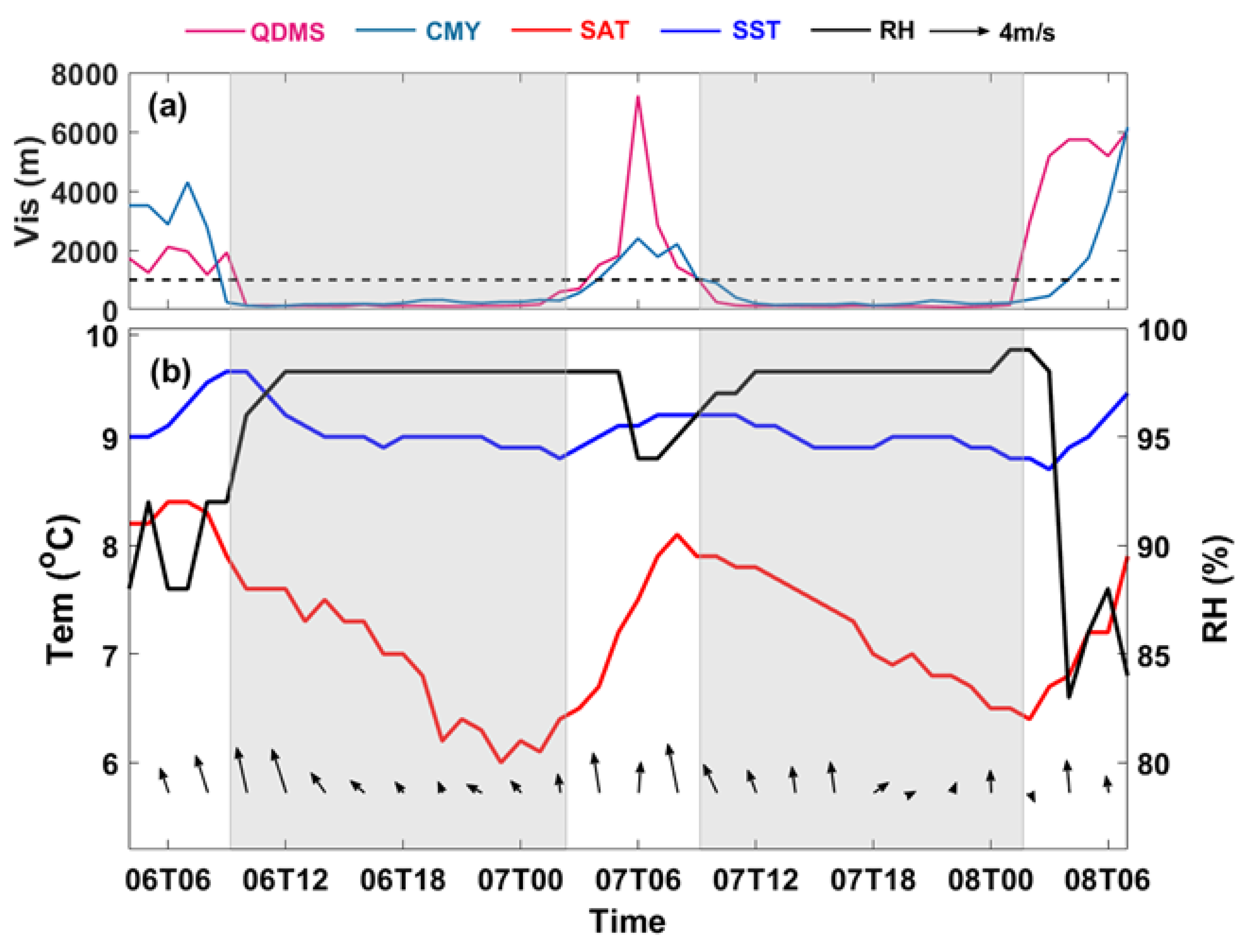
• The fog event began at around 0827 UTC 6 April 2017, and dissipated at 0230 UTC 8 April 2017 (LST = UTC + 8 h). From 0930 UTC 6 April to 0039 UTC 7 April and from 1000 UTC 7 April to 0109 UTC 8 April, the visibility remained below 200 meters, and the two fog periods lasted 31 h together. The mean value of the average LWC was 0.057 g/m^−3, and the mean value of NUM was 64.4 cm⁻³.
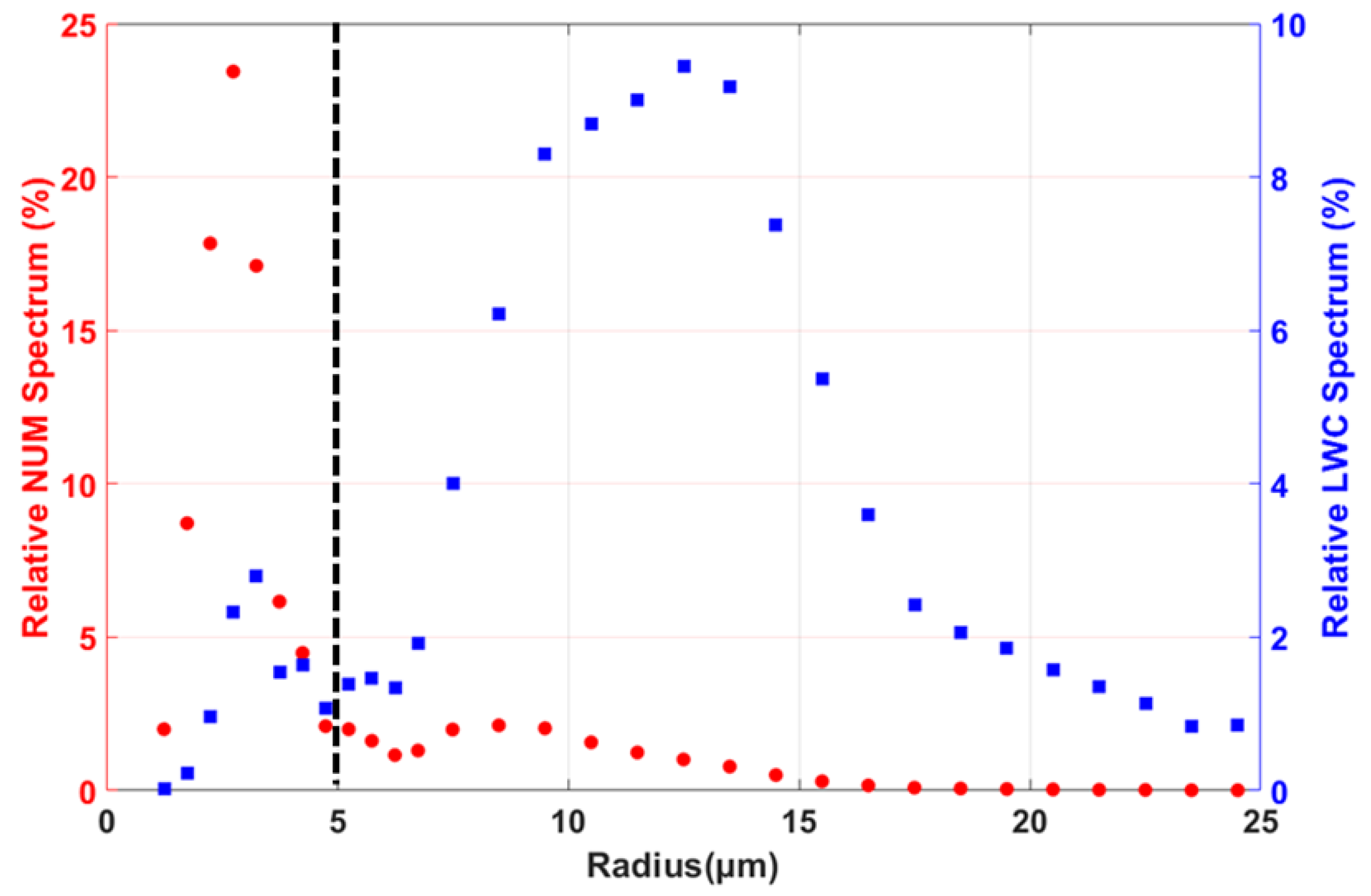
• The small droplets (radius less than 5 μm) have a decisive influence on the total NUM (the contribution of the small droplets to the total NUM is 84.84%), and large droplets (radius greater than 5 μm) have a decisive influence on the total LWC (the contribution of the large droplets to the total LWC is 93.16%).
• The observed DSD can be described well by the Gamma distribution but exhibits a bimodal distribution. We propose a G-exponential distribution function, which can describe the DSD more accurately.
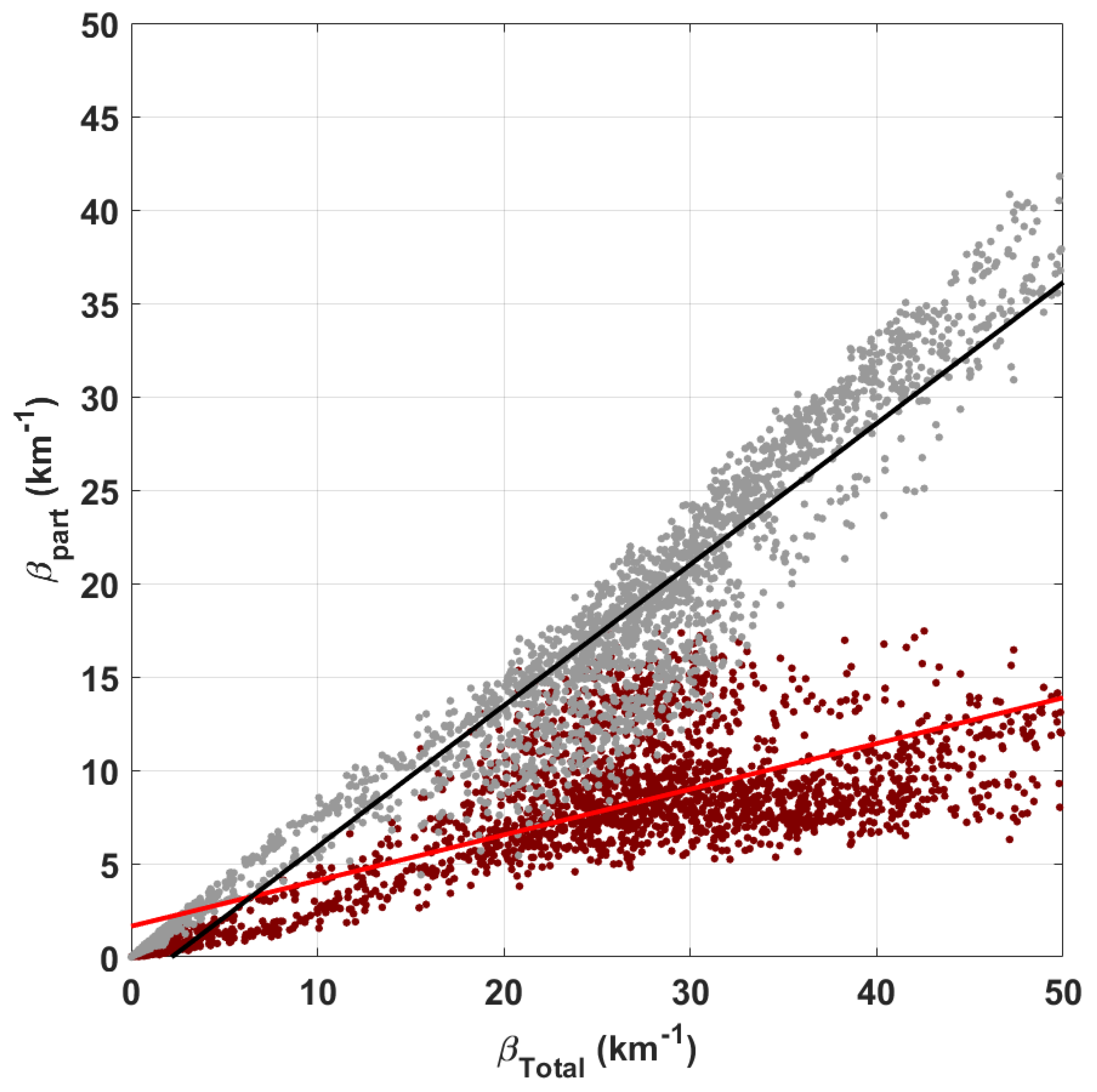
• The large droplets (radius greater than 5 μm) have a higher effect to attenuation of visibility than small droplets (radius less than 5 μm), as the contribution of the large droplets to the ${\mathsf{\beta }}_{\mathrm{ext}}$ in the whole spectra is 75.54%.
• The new visibility parameterization can improve visibility estimation, validated by the sea-fog event with the result that the $Vi{s}_{Gex}$ performs best (the smallest MAE) compared with $Vi{s}_{k84}$ and $Vi{s}_{Gamma}$.

This study shows the microphysical properties of the sea fog observed along the west coast of the Yellow Sea and gets detailed microphysical parameterizations for visibility estimation. While the results are based on just one fog event and are observed in situ on the coast, an accidental deviation may happen. The aerosol might have an impact on NUM and LWC during this coastal-fog event, while we did not discuss it here. To overcome the problems above, we will continue our observations utilizing more comprehensive instruments in offshore observation platform.

References

- Wang, B.H. Sea Fog; China Ocean Press: Beijing, China, 1985; p. 330. [Google Scholar]
- Lewis, J.M.; Korčin, D.; Redmond, K.T. Sea fog research in the United Kingdom and United States: A historical essay including outlook. Bull. Am. Meteor. Soc. 2004, 85, 395–408. [Google Scholar] [CrossRef] [Green Version]
- Gultepe, I.; Tardif, R.; Michaelides, S.C.; Cermak, J.; Bott, A.; Bendix, J.; Müller, M.D.; Pagowski, M.; Hansen, B.; Ellrod, G.; et al. Fog research: A review of past achievements and future perspectives. Pure Appl. Geophys. 2007, 164, 1121–1159. [Google Scholar] [CrossRef]
- Koračin, D.; Dorman, C.E.; Lewis, J.M.; Hudson, J.G.; Wilcox, E.M.; Torregrosa, A. Marine fog: A review. Atmos. Res. 2014, 143, 142–175. [Google Scholar] [CrossRef]
- Croft, P.J.; Pfost, R.L.; Medlin, J.M.; Johnson, G.A. Fog forecasting for the southern region: A conceptual model approach. Weather Forecast. 1997, 12, 545–556. [Google Scholar] [CrossRef]
- Gultepe, I.; Milbrandt, J. Microphysical observations and mesoscale model simulation of a warm fog case during FRAM project. Pure Appl. Geophys. 2007, 164, 1161–1178. [Google Scholar] [CrossRef]
- Eldridge, R.G. The relationship between visibility and liquid water content in fog. J. Atmos. Sci. 1971, 28, 1183–1186. [Google Scholar] [CrossRef] [Green Version]
- Roach, W.T. On the effect of radiative exchange on the growth by condensation of a cloud or fog droplet. Q. J. R. Meteorol. Soc. 1976, 102, 361–372. [Google Scholar] [CrossRef]
- Gultepe, I.; Müller, M.D.; Boybeyi, Z. A new warm fog parameterization scheme for numerical weather prediction models. J. Appl. Meteorol. 2006, 45, 1469–1480. [Google Scholar] [CrossRef]
- Elias, T.; Haeffelin, M.; Drobinski, P.; Gomes, L.; Rangognio, J.; Bergot, T.; Chazette, P.; Raut, J.C.; Colomb, M. Particulate contribution to extinction of visible radiation: Pollution, haze and fog. Atmos. Res. 2009, 92, 443–454. [Google Scholar] [CrossRef]
- Kunkel, B.A. Parameterization of droplet terminal velocity and extinction coefficient in fog models. J. Clim. Appl. Meteorol. 1984, 23, 34–41. [Google Scholar] [CrossRef] [Green Version]
- Liu, Y. Statistical theory of the Marshall-Palmer distribution of raindrops. Atmos. Environ. 1993, 27, 15–19. [Google Scholar]
- Liu, Y.; You, L.; Yang, W.; Liu, F. On the size distribution of cloud droplets. Atmos. Res. 1995, 35, 201–216. [Google Scholar] [CrossRef]
- Niu, S.; Lu, C.; Liu, Y.; Zhao, L.; Lu, J.; Yang, J. Analysis of the microphysical structure of heavy fog using a droplet spectrometer: A case study. Adv. Atmos. Sci. 2010, 27, 1259–1275. [Google Scholar] [CrossRef]
- Schmitt, C.G.; Stuefer, M.; Heymsfield, A.J.; Kim, C.K. The microphysical properties of ice fog measured in urban environments of Interior Alaska. J. Geophys. Res. 2013, 118, 11136–11147. [Google Scholar] [CrossRef]
- Zhang, S.P.; Xie, S.P.; Liu, Q.Y.; Yang, Y.Q.; Wang, X.G.; Ren, Z.P. Seasonal variations of yellow sea fog: Observations and mechanisms. J. Clim. 2009, 2, 6758–6772. [Google Scholar] [CrossRef]
- Goodin, D.S. The Cambridge Dictionary of Statistics; Cambridge University Press: Cambridge, UK, 2006. [Google Scholar]
- Draper, N.R.; Smith, H. Applied Regression Analysis, 2nd ed; John Wiley and Sons: New York, NY, USA, 1981. [Google Scholar]
- Yang, L.; Liu, J.W.; Ren, Z.P.; Xie, S.P.; Zhang, S.P.; Gao, S.H. Atmospheric Conditions for Advection-Radiation Fog over the Western Yellow Sea. J. Geophys. Res. 2018, 123, 5455–5468. [Google Scholar] [CrossRef]
- Liu, Q.; Wu, B.G.; Wang, Z.Y.; Hao, T.Y. Fog Droplet Size Distribution and the Interaction between Fog Droplets and Fine Particles during Dense Fog in Tianjin, China. Atmosphere 2020, 11, 258. [Google Scholar] [CrossRef] [Green Version]
- Hsieh, W.C.; Jonsson, H.; Wang, L.P.; Buzorius, G.; Flagan, R.C.; Seinfeld, J.H.; Nenes, A. On the representation of droplet coalescence and autoconversion: Evaluation using ambient cloud droplet size distributions. J. Geophys. Res. 2009, 114. [Google Scholar] [CrossRef] [Green Version]
- Liu, Y. Skewness and kurtosis of measured raindrop size distributions. Atmos. Envrion. 1992, 26, 2713–2716. [Google Scholar]
- Koschmieder, H. Theorie der horizontalen Sichtweite. Beitrage zur Physik der freien Atmosphare. Meteorol. Z. 1925, 12, 33–53. [Google Scholar]
- McCartney, E.J. Optics of the Atmosphere: Scattering by Molecules and Particles; John Wiley and Sons, Inc.: New York, NY, USA, 1976; pp. 1–421. [Google Scholar]
- Lentz, W.J. Generating Bessel functions in Mie scattering calculations using continued fractions. Appl. Opt. 1976, 15, 668–671. [Google Scholar] [CrossRef] [PubMed]
- Wiscombe, W.J. Improved Mie scattering algorithms. Appl. Opt. 1980, 19, 1505–1509. [Google Scholar] [CrossRef] [PubMed]
- Shen, J.Q.; Liu, L. An improved algorithm of classical Mie scattering calculation. China Powder Sci. Technol. 2005, 11, 45–50. (In Chinese) [Google Scholar]