Article

Experimental Assessment of Dust Emissions on Compacted Soils Degraded by Traffic

by
Mickael Le Vern
1,*,
Ouardia Sediki
1,
Andry Razakamanantsoa
1,
Frédéric Murzyn
2 and
Frédérique Larrarte
3
1
Department of Geotechnics, Environment, Natural Risks and Earth Sciences, University Gustave Eiffel, Allée des Ponts et Chaussées, 44340 Bouguenais, France
2
Department of Mechanical Engineering, ESTACA West Campus, Rue Georges Charpak, 53000 Laval, France
3
Department of Geotechnics, Environment, Natural Risks and Earth Sciences, University Gustave Eiffel, Boulevard Newton, 77447 Marne La Vallée, France
*
Author to whom correspondence should be addressed.
Atmosphere 2020, 11(4), 369; https://doi.org/10.3390/atmos11040369
Submission received: 12 February 2020 / Revised: 19 March 2020 / Accepted: 8 April 2020 / Published: 10 April 2020
(This article belongs to the Special Issue Wake Flows and Air Quality in the Atmosphere)

Abstract

:
Haul traffic on earthworks runways during construction works is an important factor of dust emission. Compacted soils surface become progressively degraded as the number of wheels passing increases. Fine particles are then segregated from the soil surface and lifted when the shear stress generated by the flow above the surface increases, leading to the worsening of air quality and reduction of visibility. Laboratory tests were performed to assess dust emissions on traffic degraded soils. Mixtures of kaolin clay and sand were compacted using a laboratory roller compactor and were degraded using a vehicle simulator. Models describing the evolutions of soil degradation and Particle Size Distribution (PSD) during traffic were established. Then, the velocity profiles above each soil sample were obtained in a wind tunnel. The experimental results were analyzed to determine the Reynolds shear stresses generated by the turbulence of the flow. PSD, degradation and stresses were implemented in the Convective Turbulent Dust Emission (CTDE) model to estimate the dust emission flux of the soils for several passes of the wheel. A comparison between results from the model and field measurements underlines that turbulence is not the main contributor to dust emissions when a vehicle is in motion.

1. Introduction

Vehicle traffic on compacted soils is one of the main contributors to particulate emission into the atmosphere. Excluding wind erosion, traffic on unpaved road accounts for almost 30% of dust emissions in the United States [1]. Circulation of haul trucks on earthworks runways generates also an important amount of dust. This is ranked as the second most common risk for many professionals of the construction industry [2]. Indeed, particles raised into suspension have both health and environmental impacts [3,4]. Moreover, a dust plume can reduce visibility [5,6], resulting in traffic hazards [7,8]. Soil watering is a good way to limit particle lift [9]. Nevertheless, it involves the use of large volumes of water. A better understanding of the unpaved roads dust emission mechanisms would help optimize soil watering.
The United States Environmental Protection Agency (USEPA) developed a model (called AP-42) to estimate PM10 (particle diameters less than or equal to 10 µm) emissions generated by vehicle traffic on unpaved roadways [10]. However, this model is purely empirical and shows significant discrepancies with in-situ measurements on rural unpaved roads [11] as well as on earthworks haul roads [12]. Studies have shown the effect of vehicle characteristics [11,13] and soil properties [14] on dust emission. These approaches, based on in-situ measurements, were mainly empirical. Therefore, the appearance of the particle by soil degradation and the associated lift are two mechanisms that are not yet sufficiently well-modeled.
To date, the most comprehensive analytical models of dust generation were developed in the context of wind erosion studies. When considering the soil-atmosphere interaction, many particles lift models are based on a threshold wind velocity friction [15,16,17]. However, this mechanism does not consider the turbulence. Therefore, it is relatively far from the process of particle entrainment by vehicle activity [14], since turbulence is often considered as the major factor influencing particles lift [11,18]. In order to quantify the dust emissions related to vehicle traffic, it, therefore, seems more relevant to use a turbulence-based model. In the present study, the model developed by Klose and Shao [19] is used as a basis to assess dust emissions.
Particles subjected to lift are generated by the abrasion of the soil surface due to repeated passes of vehicles [20]. However, based on the literature review, the process of soil surface degradation by tires has not yet been studied.
The preliminary aim of this study is to characterize experimentally the compacted soil degradation by traffic. The processes of particle generation and particle size evolution are studied. Three clay mixtures with different sand content were compacted using a laboratory roller compactor. Compacted soil samples were then degraded by a wheel in a traffic simulator. Stresses experienced by earthworks runways during truck circulation were reproduced. Models to quantify the evolution of soil degradation and Particle Size Distribution (PSD) during traffic were established.
The second objective of this study is to examine the interaction of the degraded soils with the atmosphere. Flow velocities were measured using LASER Doppler Velocimetry (LDV) at various locations above the soil samples in a wind tunnel. Reynolds shear stresses were determined near the soil surface to assess the lift forces experienced by the dust particles.
Degradation and PSD evolutions, as well as the particle cohesion and lift forces, were implemented into the Klose and Shao’s model [19], in order to quantify the dust emission of the traffic degraded soils.
In Section 2, the convective turbulent dust emission model and the related assumptions are detailed. In Section 3, experimental facilities and measurement techniques are presented. In Section 4, the results are detailed and discussed. In the last section, conclusions and perspectives are presented.

2. Convective Turbulent Dust Emission Model

2.1. Description of the Klose and Shao’s Model

Convective Turbulent Dust Emission (CTDE) model establishes that particle lift initiate when interparticle cohesive forces become smaller than lifting forces generated by turbulence [19]. According to a force balance, the emission flux φd (kg·m−2·s−1) of particles having a diameter d can be expressed as Equation (1):
φ d = { N d T p 2 ( f f i d δ v c )   f o r   f > F i   a n d   δ v c > d 0                                                           e l s e ,
where Nd is the particle number concentration per unit of volume (m−3), Tp is the particle response time (s), f is the lifting force expressed in newtons (N), fi is the interparticle cohesive force (N) and δvc is the thickness of the viscous sublayer area where the particles are sheared. δvc is given by Equation (2):
δ v c = 5 ν u * ,
with ν being the air kinematic viscosity (15.6 × 10⁻⁶ m2·s−1 at 25 °C) and u* the friction velocity (m·s−1).
According to [21], Tp is given by Equation (3):
T p = 1 18 d 2 ν ρ p ρ ,
with ρ p being the particle density (kg·m−3) and ρ the air density (1.184 kg·m−3 at 25 °C).
The force exerted on the particle is given by Equation (4):
f = | τ | · π d 2 4 ,
where τ is the Reynolds shear stress, that is, the instantaneous vertical flux of horizontal momentum given by Equation (5):
| τ | = ρ ( u v ) 2 + ( v w ) 2 .
In Equation (5), u′, v′ and w′ are, according to the Reynold decomposition, the instantaneous fluctuations of the flow velocity (m·s−1) in the longitudinal, vertical and spanwise directions respectively. These fluctuations depend on time, so the Reynolds shear stresses are not constant. Thus, τ is a stochastic quantity that obeys a probability distribution p(τ) depending on the Probability Distribution Functions (PDF) of u′, v′ and w′.
The cohesive force (fi) mainly depends on the Van der Walls interactions, electrostatic forces as well as capillary and chemical binding forces [21]. These interactions are affected by many parameters including, but not limited to, the particle size, the particle shape, the mineral composition and the surface roughness. Therefore, cohesive forces are difficult to estimate. It is more convenient to treat these forces as stochastic variables following a probability distribution p(fi). Finally, according to [19], the total convective dust emission flux can be given by Equation (6):
φ = d m i n d m a x [ 0 ( 0 f φ d · p ( f i ) d f i ) p ( f ) d f ] p ( d ) δ d ,
where p(d) is the PSD of the soil and p(f) is the probability distribution of f.
This model has shown a good ability to predict dust emissions during atmospheric convective turbulent events in Taklimakan Desert (China), Horqin Sandy Land (China) and in the Murray-Darling River Basin (Australia). Coefficients of determination (r2) up to 0.71 were obtained when comparing model predictions with observations both at a site-based scale [22,23] and a regional scale [24].
In the present study, the originality of the approach is to use this model to quantify dust emissions on traffic degraded soils. Input parameters to be implemented in the model are: PSD, the quantity of particles and probability distributions of cohesive and lifting forces. The following section details the determination of these parameters.

2.2. Determination of the Model Input Parameters

2.2.1. Particle Size Distribution (PSD) and Quantity of Particles Subjected to Lift

The PSD of soil can be obtained by sedimentation [25], sieving [26] or by techniques such as LASER diffraction [27]. The latter technique was used in the present study. In the context of dust emission by vehicle-induced traffic, the PSD of soil particles that get lifted is different than the PSD of the initial soil. Indeed, due to the soil moisture content and the compaction load, compacted soil is composed of particles bonded together to form aggregates. These aggregates are pulled out of the compacted soil surface under the shearing action of a wheel rolling over the surface [28]. The PSD of these aggregates is comparatively coarser than that of the initial soil. By increasing the number of wheel passing, finer particles are formed by aggregate crumbling. This leads to an evolution of PSD over time. In the same way, the number of particles segregated from the surface evolves as the soil degradation by traffic increases. The experimental approach for the study of PSD and degradation evolutions during traffic is detailed in Section 3.1.

2.2.2. Cohesive Forces

The stochastic behavior of interparticle cohesive forces was dealt with in the study of Zimon [29]. The experiments were performed with glass particles submitted to a centrifugal acceleration to induce their flight. By gradually increasing the centrifuge force and measuring the proportion of particles lifted, the statistical distribution of cohesive forces was estimated. According to the results obtained, the cohesive force can be described using a log-normal distribution defined by Equation (7):
p ( f i ) = 1 f i 2 π σ f i exp ( ( l n f i l n f i ¯ ) 2 2 σ f i 2 ) ,
where f i ¯ is the median value of the cohesive force (fi) and σ f i its geometric standard deviation (N).
The log-normal distribution for cohesive forces is also proposed by other researchers for other types of particles [30,31,32]. Dealing with Zimon’s data, Shao [21] proposed an empirical law to estimate f i ¯ and σ f i as a function of particle size (Equation (8)):
f i ¯ ( d ) = 10 8 ( 10 × e 4.3569 0.2183 d + 0.0018 d 2 ) 1
σ f i = 10 8 ( 4.1095 0.0476 d ) ,
where d is expressed in μm.
Figure 1 shows the distributions of fi for particles having diameters of 1 μm, 2 μm, 3.5 μm, 7.5 μm and 20 μm. The geometric standard deviation for the log-normal distribution σ f i is inversely proportional to the particle diameter. The distribution functions p(fi) cover a wide range for fine particles, demonstrating the need to consider the stochastic behavior of cohesive forces when examining dust emission.

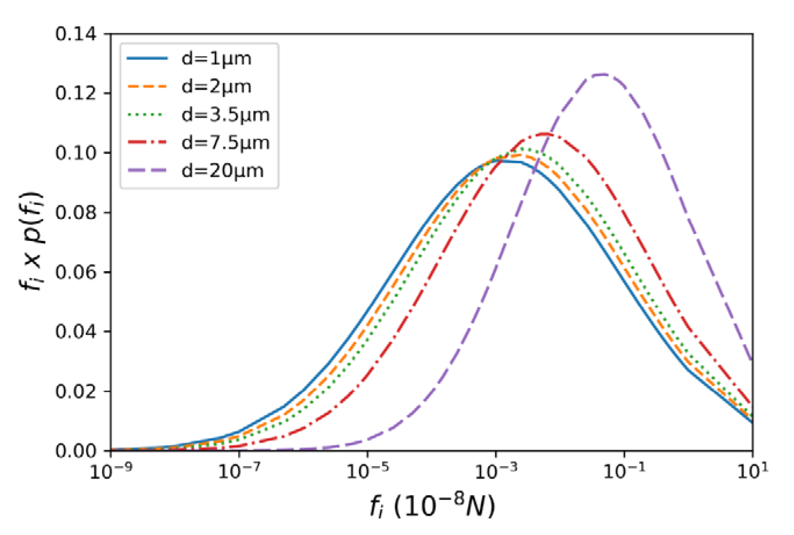
2.2.3. Lifting Forces

Lifting forces due to the wind were determined through wind tunnel experiments by measuring velocities of the air above traffic-degraded soils (Section 3.2). However, for practical reason, only the longitudinal component u′ was measured. In order to assess the Reynolds shear stresses, assumptions about vertical and transverse fluctuations were made and discussed below.
For simplification in the study, it is assumed that turbulence is isotropic (u′ = v′ = w′). In reality, the presence of a mean flow orientated in horizontal direction introduce anisotropies in the turbulent velocity, the longitudinal fluctuation u′ being greater than other fluctuations. Thus, an idealised turbulent state is considered that overestimates the Reynolds shear stresses (conservative hypothesis). It is worth noting that this assumption is often used in numerical models [33,34,35]. Reynolds shear stresses are therefore expressed in a simpler way Equation (10):
| τ | ( u = v = w ) = ρ ( u u ) 2 + ( u u ) 2 = 2 ρ u u ,
where τ is the product of two variables, both having a distribution function pu′. Thus, the Reynolds shear stresses distribution function p(τ) is a product distribution [36] (p. 160), given by Equation (11):
p ( τ ) = 2 ρ + p u ( x ) . p u ( τ / x ) · 1 | x | d x
where x is the set of values that can be taken by u′.
In the next section, the experimental facilities and measurements techniques are described.

3. Experimental Facilities and Measurement Techniques

3.1. Compaction and Degradation of the Soil Samples

3.1.1. Compaction

In civil engineering, soils are compacted to improve their bearing capacity [37]. A good quality of compaction is particularly important for soils submitted to stresses induced by vehicle traffic, such as unpaved roads or runways on earthworks site. In this study, soils were compacted using the roller compactor of the University Gustave Eiffel (Figure 2). This device allows reproducing the stress tensor rotation in the soil during compaction, which is similar to field conditions [38].
Soil samples were prepared with mixtures of two materials: Kaolin clay (defined as K) and Hostun HN38 sand (defined as S). Three different mixtures were studied: a pure clay sample S0K100 (100% of clay) and two different sand-clay mixtures S50K50 (50% of clay and 50% of sand) and S75K25 (25% of clay and 75% of sand). These three soil mixtures cannot fully represent natural soils but are representative of the fine soils encountered usually on construction sites, and thus chosen herein. According to the French guide of road earthworks [39], S0K100 is classified A3 (medium-plastic clay), S50K50 is classified A2 (fine clayed sand) and S75K25 is classified A1 (fine sand). The PSD of the samples was measured by LASER diffraction (Section 3.1.2). These soils were compacted in 500 × 180 × 28.5 mm3 rectangular samples. The compacting process consisted of pouring the required quantity of soil to be compacted into the container placed inside the base. A displacement table gradually lifted the container while a smooth wheel moved over the surface until the soil was compacted to a height of 28.5 mm in the container.
Five samples (1 of S0K100, 1 of S50K50 and 3 of S75K25) were compacted at the Proctor optimum, which is the optimum moisture content for maximum soil density after compaction [40]. The compaction parameters are detailed in Table 1. After compaction, the soils were air-dried for 24 h and then degraded with a tire in a traffic simulator. All the tests were carried out during summer under the same weather conditions (approximately 25 °C during compaction and degradation).

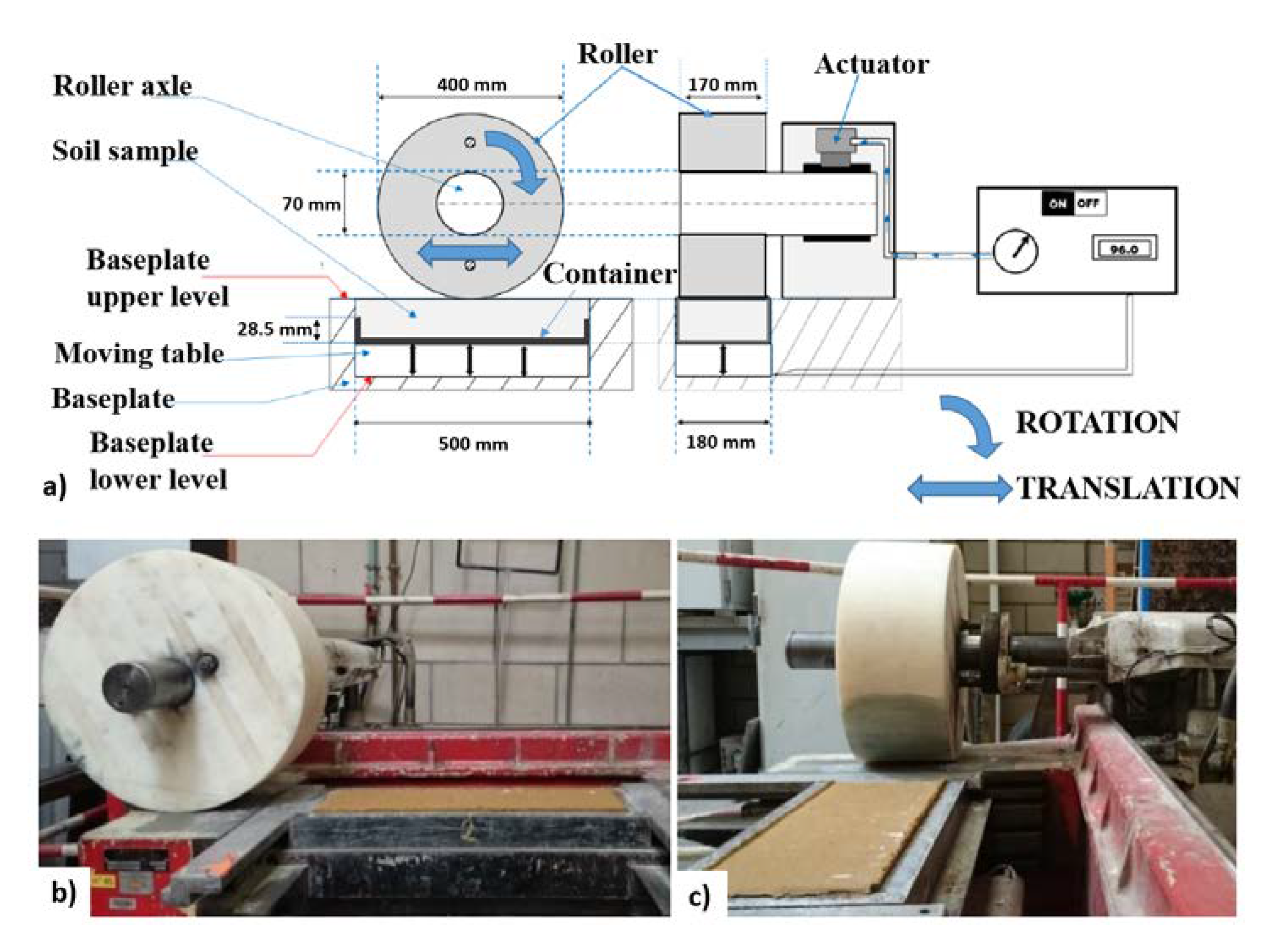
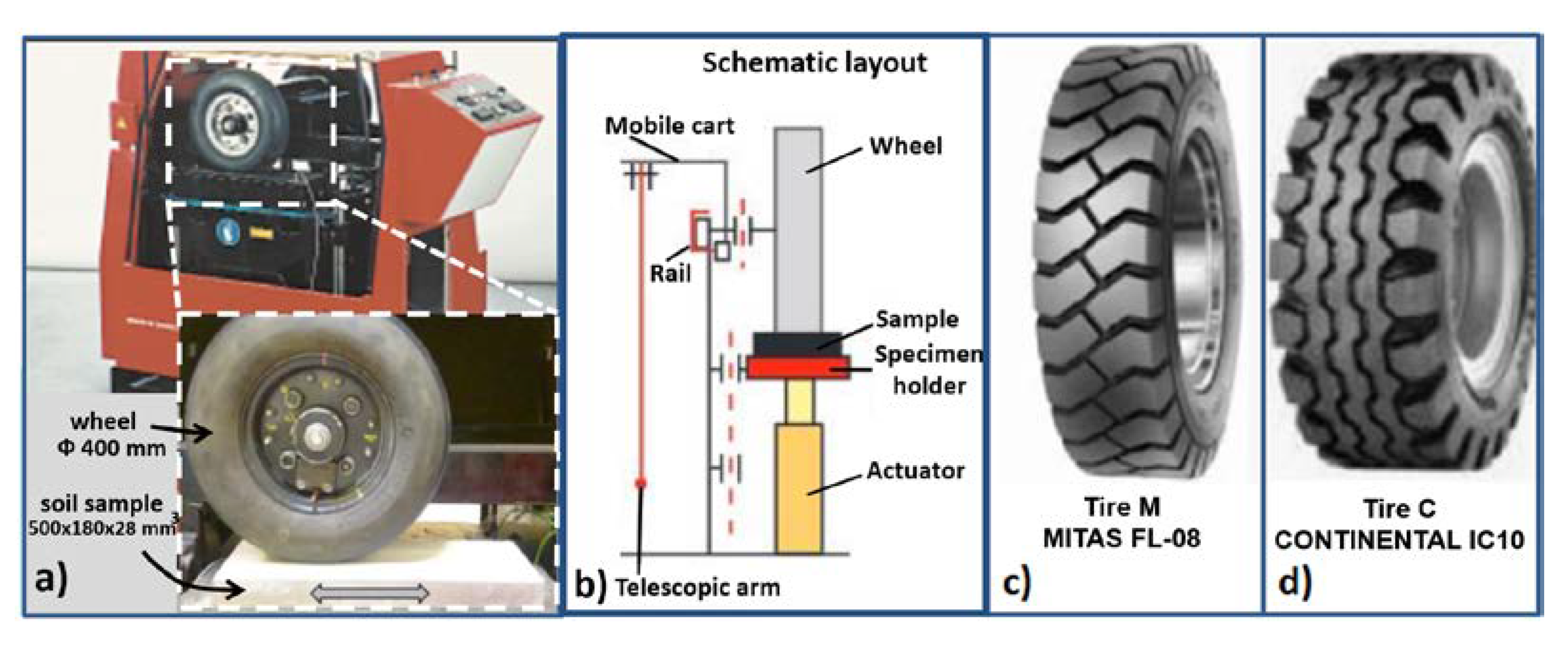
3.1.2. Soil Degradation by Traffic Simulation

After compaction, the soil samples were degraded in the traffic simulator VECTRA at the University Gustave Eiffel. This apparatus (Figure 3a) simulates the motion of a wheel equipped with a 400 mm diameter tire. The movement is generated according to the following procedure: the continuous rotation of a gear motor unit is transformed into a reciprocating movement by an oscillating bearing carrying a telescopic arm. This arm transmits its movement to a mobile carriage that is mounted on a rail. The wheel is fixed to this mobile carriage and moves longitudinally along the axis of the rail by reciprocating passes over a distance of 0.410 ± 0.005 m with a frequency of 1.0 ± 0.1 Hz (Figure 3b). This corresponds to an average speed of approximately 4 km/h, which is the speed limit of the apparatus. Such a low speed induces a longer contact between the wheel and the ground. As a consequence, the normal stress distribution is greater in the soil samples than it would have been in the field [41], but the frictional stress is lower.
This apparatus is generally used to study the rutting of bituminous materials with a smooth-tire. The present tests were devoted to the study of the degradation of soil with sculpted tires. This is the novelty and the originality of the present study. Two tires (Mitas FL-08 and Continental IC 10, named M and C, respectively) were used during the tests (Figure 3c,d). They were inflated to a pressure of 600 kPa as specified by the manufacturer. The contact action of the tire on the ground was achieved by means of an actuator located under the sample. The pressure applied by the actuator was 320 kPa (minimum value of the device), which corresponds to a tire/ground contact pressure of 898 kPa for the Mitas FL-08 tire and 753 kPa for the Continental IC10 tire. These contact pressures did not consider the penetration of the tire into the ground. They were assessed by dividing the contact force by the contact area with a plate. The simulated contact pressures were between 2 and 4 times higher than the non-penetrating contact pressures of Michelin XADN tires, which are used on many articulated dump trucks and varying between 200 and 400 kPa for conventional loads [42]. The tests carried out reproduced, therefore, the movement of rubber tires on the soil with three main scale effects: high stresses, low driving speeds and no engine torque.
Samples I–V were subjected to a total number of 20,000 wheel passes while sample IV underwent 10,000 passes (Table 1). These numbers of passes were chosen to simulate the similar soil stress that can be expected on a construction site over a long period of time (one month approximately). This was defined according to Midwest Research Institute measurements at four earthmoving sites in the United States [43], assuming between 100 and 200 truck passes per day (i.e., between 2000 and 4000 passes per month). Considering three wheel passes per truck (an articulated dump truck has three wheels on each side), it leads to about 10,000 wheel passes per month. The Midwest Research Institute’s estimates were carried out on construction sites during periods of low activity [43]. It is assumed that the soil on a construction site during a period of high activity can be subjected to at least twice as much truck traffic (i.e., 20,000 wheel passes).
For each sample, the traffic simulator was stopped after 20, 60, 120, 200, 300, 400, 500, 600, 800, 1000, 2000, 4000 and 10,000 wheel passes. At each stop of the device, the particles detached from the soil were collected by lightly sweeping the surface with a fine brush and subsequently weighed. The evolution of the mass of the removed particles allows the quantification of soil degradation by traffic cycles. The particles detached after 20,000 wheel passes for samples I and II were placed in a LASER diffractometer to measure their PSD. Similarly, the particle sizes after 2000, 10,000 and 20,000 passes on sample III were also measured. The corresponding PSD was measured according to ISO 13,320 [27] and are presented in Section 4.1.2.

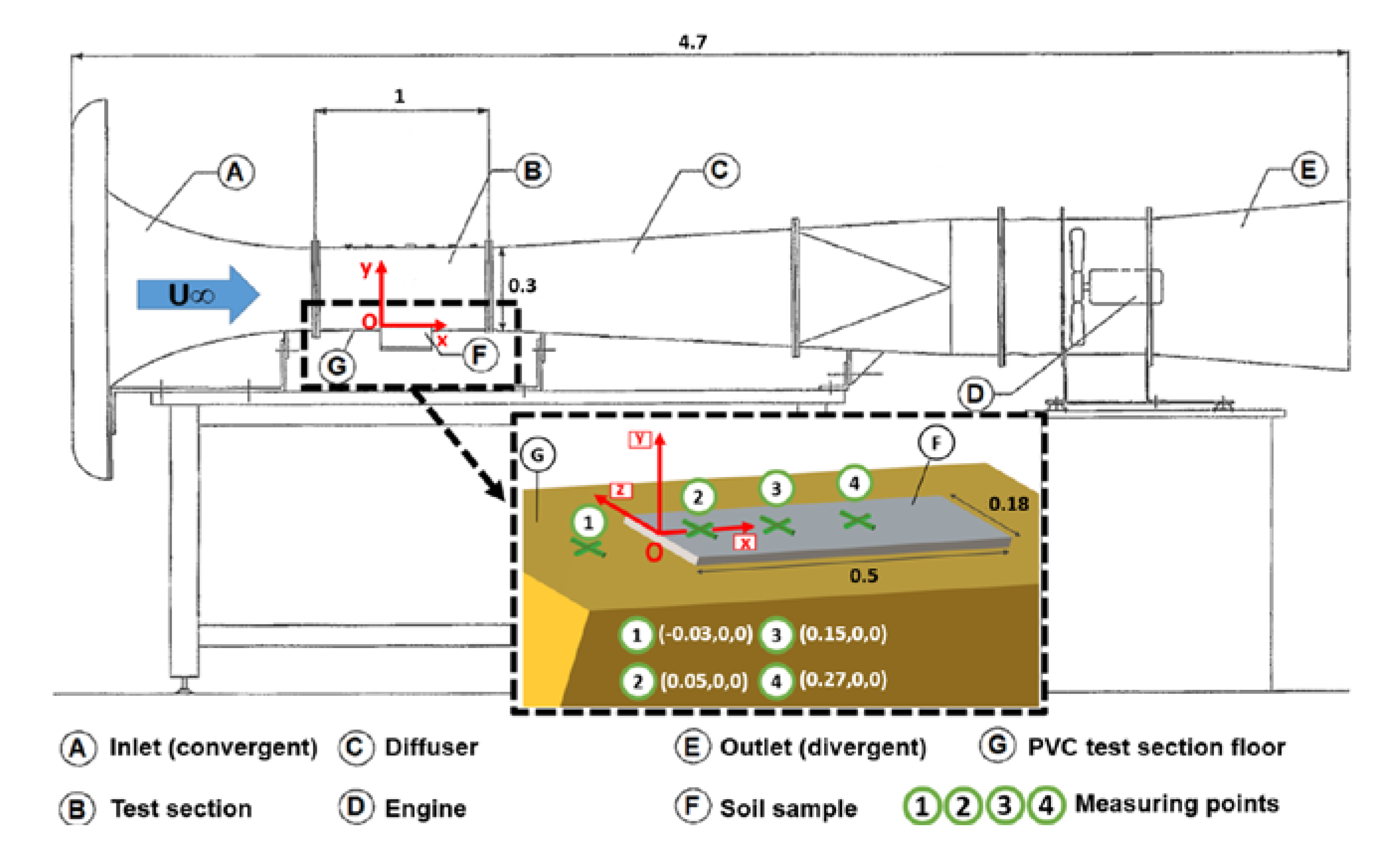
3.2. Soil-Atmosphere Interaction: Wind Tunnel Experiments

After compaction and traffic degradation, samples I, III, IV and V were placed in a wind tunnel and the airflow above the soil was investigated. For this purpose, the boundary layer was characterized. The tests were carried out in the subsonic wind tunnel at ESTACA West Campus (Figure 4). The test section had a squared cross-section of 0.3 × 0.3 m2 and was 1 m long. The airflow was generated by a 3 kW engine. The mean turbulence intensity in the test section outside the boundary layer was low (<1%). Before wind tunnel experiments, the soil samples were sprayed with a lacquer (StruersTM) to prevent the boundary layer from being disrupted by dust emissions. Roughness measurements with a rotating LASER profilometer before and after lacquer application showed that this did not alter the surface roughness.
Velocity measurements were recorded using a 2D LASER velocimeter provided by DANTEC® Dynamics. This system was mounted on a 3D displacement table. Two upstream flow velocities were considered (U = 8 m·s−1 et U = 16 m·s−1). They were defined to fit with typical truck speeds on construction sites (between 30 and 60 km·h−1). The coordinate system was such that x corresponded to the horizontal axis (positive downstream), y and z being the vertical (positive upward) and spanwise (positive from the left to the right looking from the entrance of the test section) directions, respectively. The origin O was taken at the center of the leading edge of the sample, on the channel centreline. The vertical profiles of the velocity were measured at the centreline (z = 0) of the test section at four given positions depicted by points 1 to 4 in Figure 4. The first point was used as a reference on the PVC floor of the wind tunnel (x = −0.03 m) while the three other points were located on the soil sample (x = 0.05, 0.15 and 0.27 m). In Figure 4, the flow is from the left to the right.
43 measurements at different vertical positions above the soil were recorded for each vertical profile (Table 2).
From a theoretical point of view, the boundary layer profile developing above the soil can be approximated using Equation (12):
u u * = 1 κ ln ( y · u * ν ) + B ,
where κ is the Van Kármán constant ( κ ≈ 0.41) et B a constant determined by experiments.
The wind friction velocity u* was determined using the method developed by Djenedi et al. [44]. It can be applied regardless of the surface roughness and the Reynolds number of the flow. By a trial-and-error method, the value of u* was found by matching each vertical velocity profile with the normalized velocity defect form given by Equation (13):
U u u * = h ( y δ ) ,
where δ is the boundary layer thickness (m) and h is a universal function that applies to all turbulent boundary layers [44] and defined by Equation (14):
h ( y δ ) = p 1 ( y δ ) 5 + p 2 ( y δ ) 4 + p 3 ( y δ ) 3 + p 4 ( y δ ) 2 + p 5 ( y δ ) + p 6 ( y δ ) 5 + q 1 ( y δ ) 4 + q 2 ( y δ ) 3 + q 3 ( y δ ) 2 + q 4 ( y δ ) + q 5 ,
where the coefficients pi (I = 1,2,…,6) and qj (j = 1, 2, …, 5) are:
p1 = 110.50, p2 = −230.50, p3 = 114.50, p4 = 7.24, p5 = −6.38 × 10⁻³, p6 = −4.60 × 10⁻⁵;
q1 = −10.07, q2 = 15.56, q3 = 4.47 × 10⁻¹, q4 = −8.20 × 10⁻⁴ and q5 = −1.79 × 10⁻⁶.
The determination of the flow regime was carried out using the shape factor H Equation (15):
H = δ * θ ,
where δ* is the displacement thickness (m) and θ is the momentum thickness (m), given by Equations (16) and (17), respectively:
δ * = 0 ( 1 u U ) d y
θ = 0 u U ( 1 u U ) d y .
The flow is turbulent if H < 1.4 and laminar if H > 2.6 [45].
From flow velocity measurements, the statistical distributions of their corresponding fluctuations were determined. The statistical distribution of Reynolds shear stresses were determined according to Equation (11). Then, for each velocity profile, the fluctuations closest to the soil were considered to apply the dust emission model (Equation (6)). This process is detailed in Section 4.3.1.

4. Results and Discussion

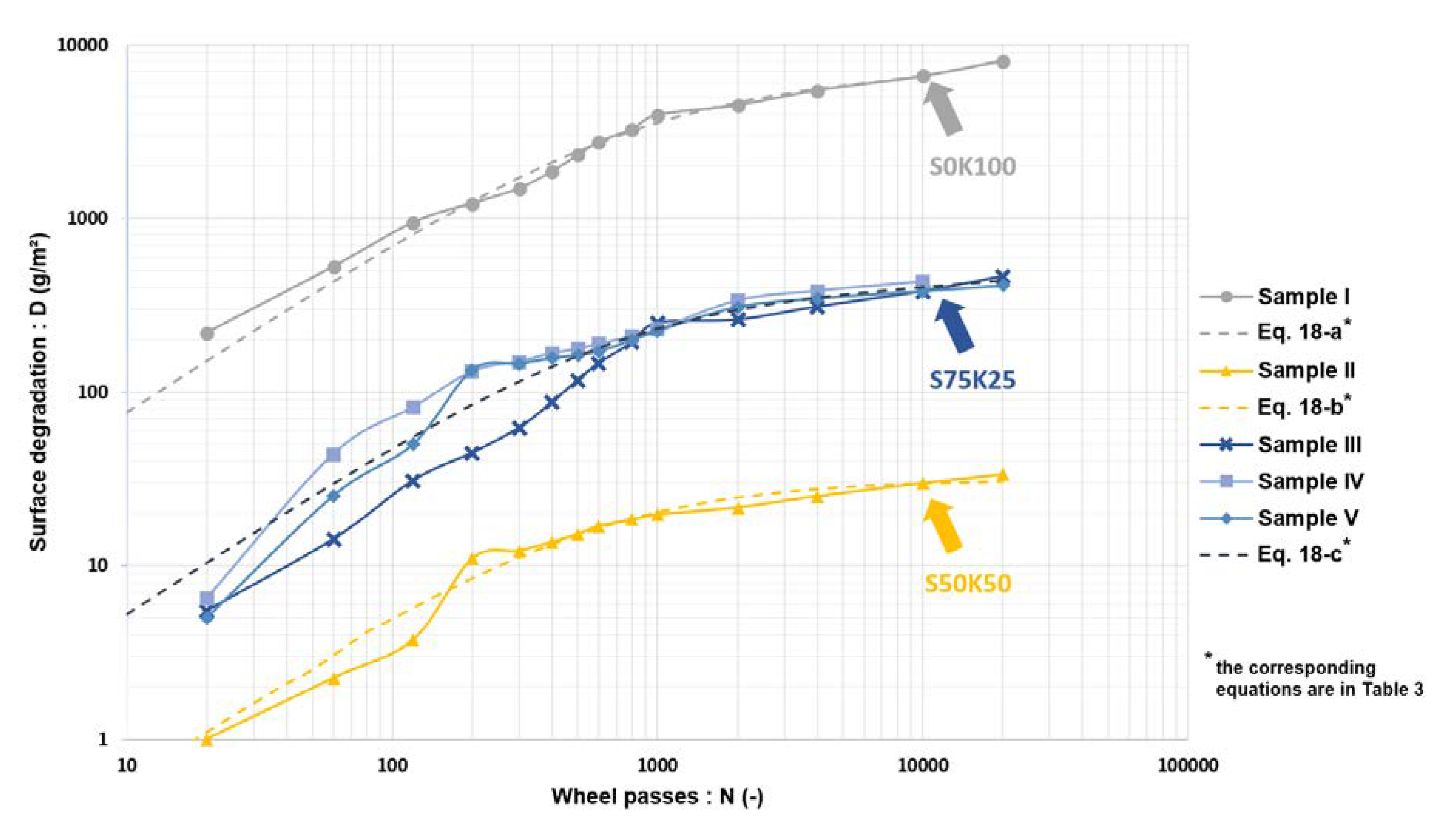
4.1. Soil Degradation by Traffic

4.1.1. Detachment of Particles from the Soil Surface

Surface degradation was quantified using the D parameter which corresponds to the cumulative mass of detached particles in relation to the ground surface covered by the tire during its movement (0.04 m2 for each tire in the present study). Figure 5 shows the evolution of D as a function of the number of wheel passes for each of the samples.
For each soil, an empirical model describing the data using the least-squares method was established according to the function (Equation (18)):
D ( N ) = c 1 N 2 + c 2 N c 3 N 2 + c 4 N + c 5 ,
where N is the number of wheel passes and ci (I = 1, 2, …, 5) are coefficients determined from the experiments and detailed in Table 3.
Figure 5 shows a good agreement between Equation (18) and the experimental data. For the S75K25 soil (samples III, IV and V), the fitting curve was plotted considering an average of the three samples. Indeed, for this soil, a good reproducibility of the experimental data on samples was obtained with the same test conditions (samples III and IV) as well as for sample V which was degraded with a different tire (Figure 5).
Overall, the behavior was the same for the three soils: a regular increase of the surface degradation with the number of wheel passes was observed, up to a certain threshold (about 200 passes) where an inflection appeared. During the first traffic cycles, the compacted soil surface seems to resist the shear generated by the tire, but gradually the tire tread pattern starts appearing on the surface. Visually, after about ten passes, the first aggregates segregated and crumbled, leading to a significant increase in soil degradation. After a few hundred cycles, the soil mainly became plasticized: fewer particles were pulled out as rutting (structural deformation) became the main mode of degradation.
The difference between the three soils relies on the quantification of degradation: after 100 wheel passes, degradation was worth several tens, several hundreds and several thousands of grams of particles per unit area for S50K50, S75K25 and S0K100 respectively. S50K50 soil had a well-graded PSD with a good balance between sand and clay. This gave a microstructure to the S50K50 sample that was not as porous as the S75K25 sample [28]. The imbalance between the amount of sand and clay in the S75K25 soil resulted in the presence of more macropores in this material. Indeed, sand particles give rise to large pores between them and S75K25 did not contain enough clay to fill those pores. Macropores are areas of weakness in the granular matrix. Their presence increases the risk of aggregate detachment. The S0K100 soil had a PSD consisting only of clay particles with low porosity. However, this soil had a shear strength which was almost 20% lower than S50K50 soil and 30% lower than S75K25 soil [38]. Thus, the S0K100 soil surface was much less resistant to the stresses generated by wheel traffic. A field test would be required to validate the degradations observed in the laboratory tests.
After studying the appearance of particles on the soil surface during traffic, the PSD of these particles is analyzed in the following section.

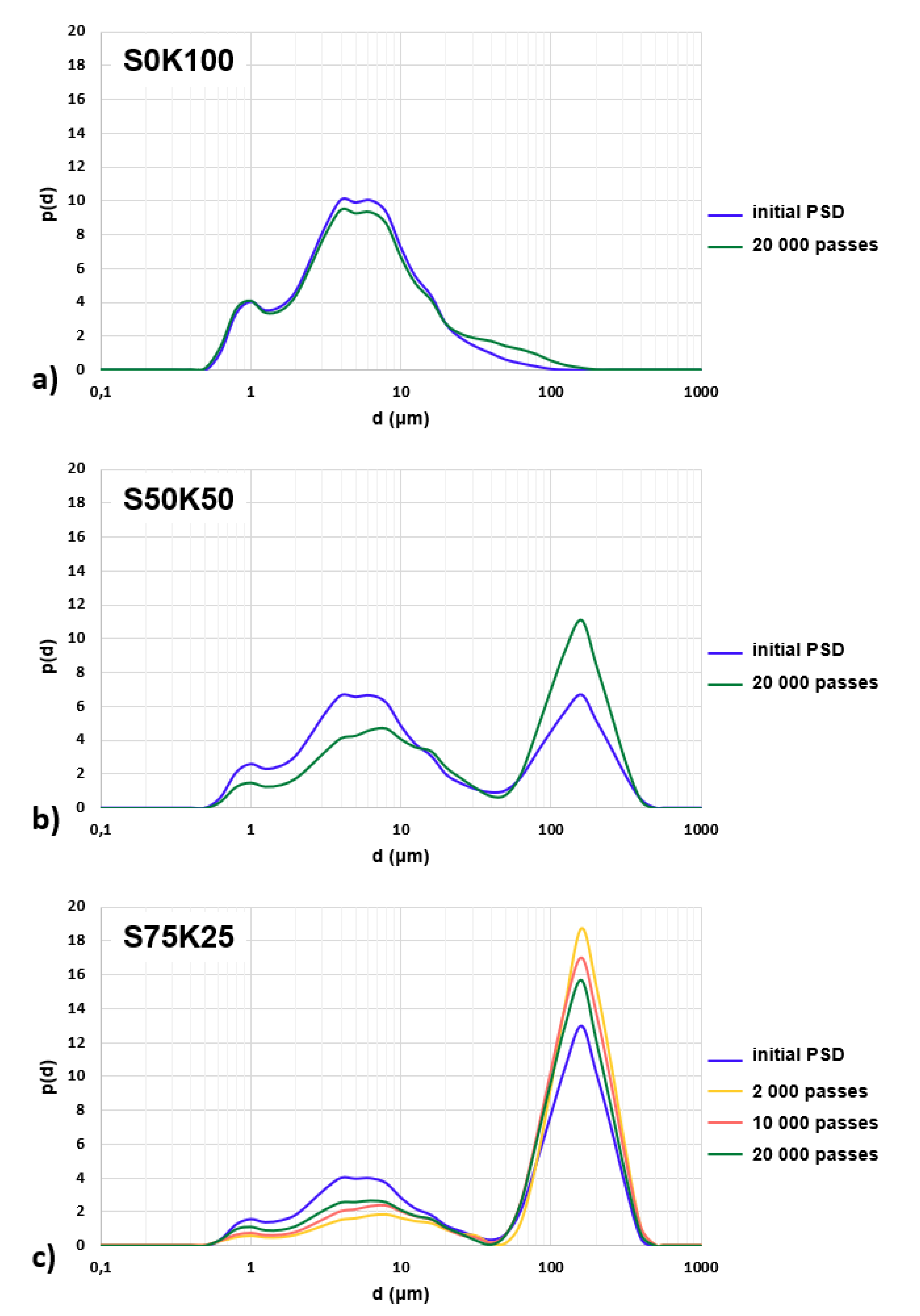
4.1.2. PSD of Particles Segregated from the Soils during Traffic Degradation

Figure 6 shows the initial PSD of the three soils and the PSD of the loose particles at 20,000 wheel passes on the S0K100 (Figure 6a) and S50K50 (Figure 6b) samples. Figure 6c shows the same curves, as well as the PSD of the loose particles at 2000 and 10,000 wheel passes on the S75K25 sample. Overall, the detached particles had a lower percentage of fine particles (<10 μm) and a higher percentage of coarse particles (>10 μm) compared to the original soil. This phenomenon was particularly marked for both soils containing sand compared to clay. This was explained by the fact that the sand and clay particles agglomerate to form coarser particles (aggregates) that were torn off by the tire. Figure 6c shows that this phenomenon of particle aggregation decreased as the number of wheel passes increased. There was, therefore, a progressive crumbling of the aggregates with the friction generated by the tire.
The gap between the PSD curves that correspond to the degraded state and to the initial state was assessed using the empirical function “difference” (Equation (19)). This function was obtained by considering the soil properties and the number of wheel passes. For more details regarding the methodology adopted, refer to the Appendix A provided at the end of the present paper.
d i f f e r e n c e = 0.111 × e [ 0.004 ( % c l a y × % s a n d ) ] 0.49 × ( 9.72 × 10 10 N 2 4.92 × 10 5   N + 1.09 ) × ln ( d d m i n ) × s i n [ 2 π ln ( d m a x d m i n ) × ln ( d d m i n ) + π ] ,
where %clay is the mass percentage of particles smaller than 2 μm and %sand is the mass percentage of particles between 20 μm and 2000 μm [46], dmin and dmax represent the minimum and maximum soil particle diameter (µm) respectively.
If the PSD of the initial soil p(d)initial soil is known, it is possible to predict the granulometry of the particles detached after N wheel passes, that is p(d)N passes (Equation (20)):
p ( d ) N   p a s s e s = { p ( d ) i n i t i a l   s o i l + d i f f e r e n c e                 f o r   d m i n d d m a x                             0                                                                                                       e l s e           .
Figure 7 compares the data provided in Figure 6 with the prediction results (dashed lines). The correlation between the model and experimental results was examined by studying the difference between the area under the model curve (p(d)model) and the area under the experimental curve (p(d)exp), according to Equation (21):
g a p m o d e l / e x p e r i e n c e = d m i n d m a x p ( d ) m o d e l δ d d m i n d m a x p ( d ) e x p δ d d m i n d m a x p ( d ) e x p δ d × 100 % .
Except for 20 μm < d < 60 μm, where the deviation between the theoretical and experimental curves were obvious for S50K50 and S75K25samples, the average deviations were 6% for S0K100 and 30% for S50K50. For S75K25, the average deviations between the model and the experimental data were 15%, 32% and 47% for 20,000 passes, 10,000 passes and 2000 passes, respectively. Overall, the model was in good agreement with the experimental results, which indicates that it was able to reproduce satisfactorily the mechanisms of degradation for the three soils.

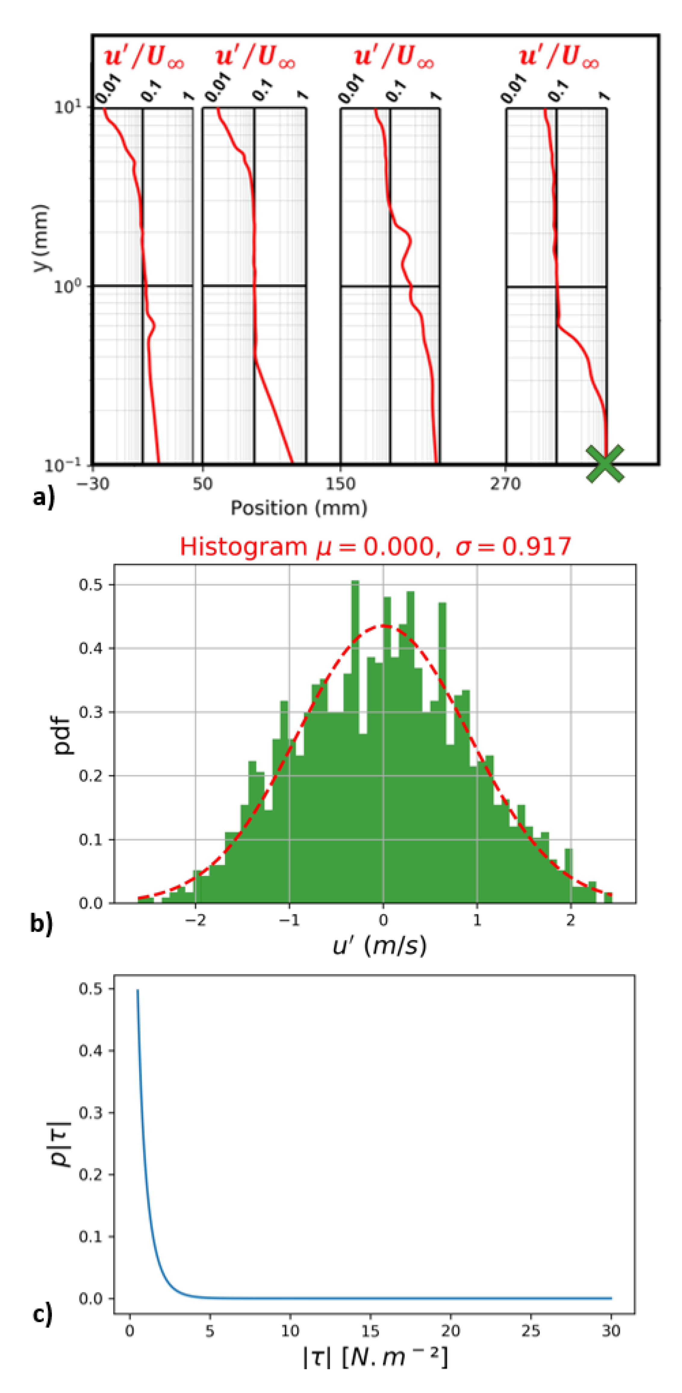
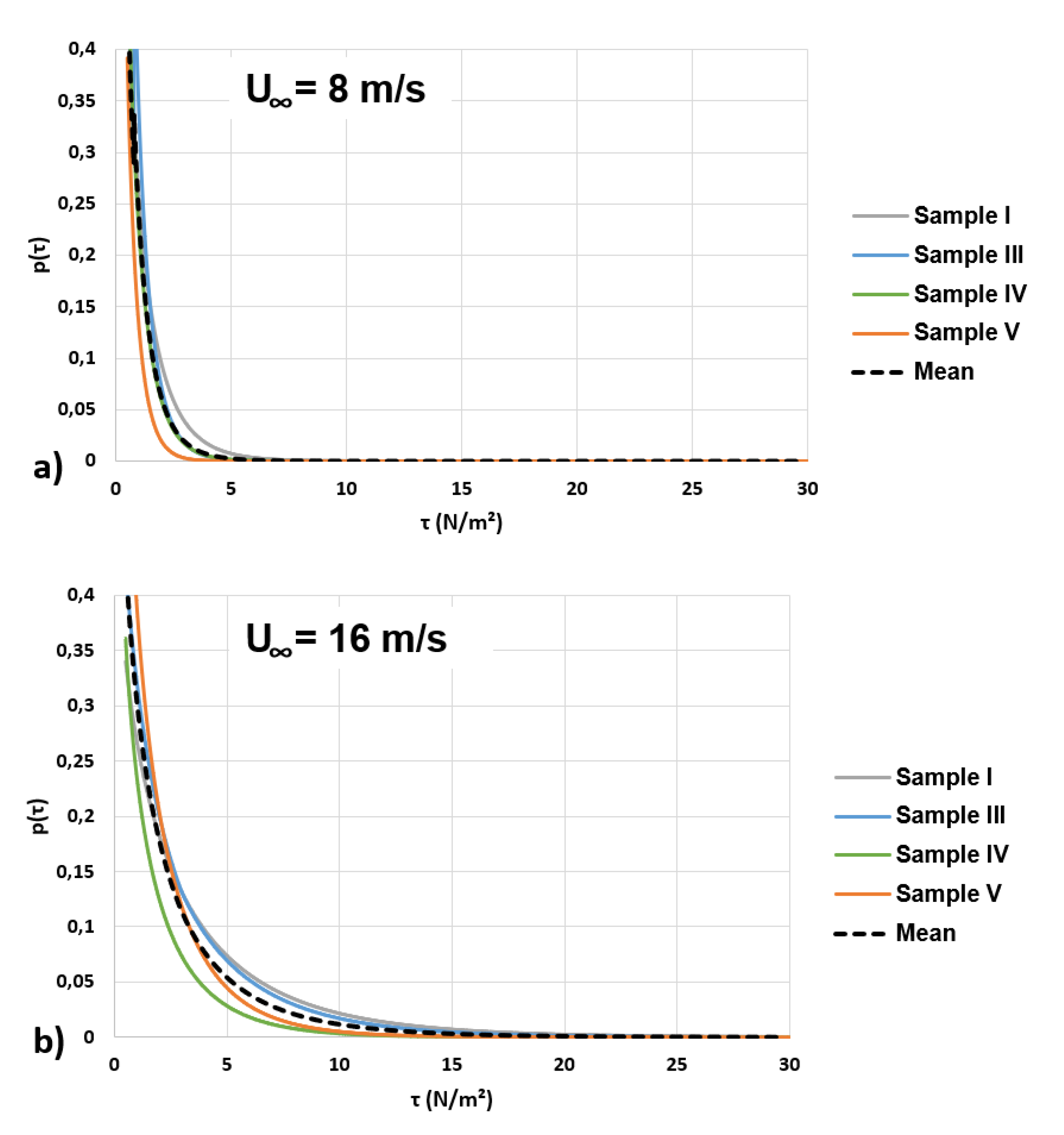
4.2. Boundary-Layer Characterization

Table 4 presents the main characteristics of the boundary layer determined from the velocity measurements (parameters H, u* and δvs calculated from Equations (15), (13) and (2), respectively). Considering H, all profiles corresponded to either a fully turbulent flow or a transitional regime.
Apart from a few situations (at positions x = 0.05 m and 0.27 m on samples IV and V), the thicknesses of the viscous sublayer were similar in terms of magnitude for the different samples considering the same inflow velocity. For the sake of simplicity, for each velocity, the mean over all values was chosen to be implemented into the dust emission estimation model. That is, δvs = 300 µm for U = 8 m/s and δvs = 135 µm for U = 16 m/s. It is worthwhile to note that a variation of 50% of this parameter in the model led to a variation of the dust flow of less than 2%.

4.3. Application of the CTDE Model

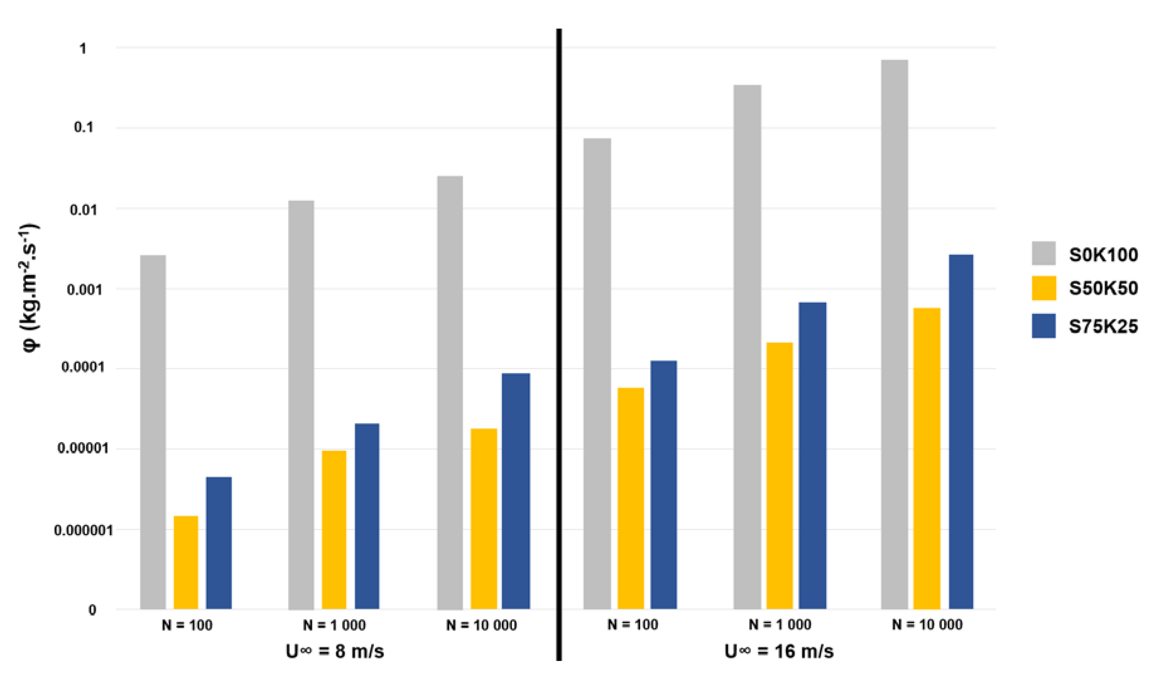
4.3.1. Estimation of Dust Emissions from Studied Soils

Wind tunnel measurements were used to determine the velocity fluctuations above the samples and to derive Reynolds shear stresses generated by the turbulence developing in the vicinity of the surface. Figure 8 shows an example of these estimated Reynolds stresses for sample IV and U = 8 m/s. Figure 8a shows the streamwise turbulence intensity above the sample. Figure 8b shows the PDF of the velocity fluctuations corresponding to the point depicted by a green cross (x = 0.27 m; y = 0.0001 m) in Figure 8a. The velocity fluctuations appeared to follow a normal distribution defined by Equation (22):
p d f ( u ) = 1 σ 2 π e 1 2 ( u μ σ ) 2 ,
where μ et σ are the median value and the geometric standard deviation of the distribution.
It was then possible to determine the PDF of τ (Figure 8c) using Equation (11). Figure 9 shows the corresponding PDF of τ for the 4 samples and for the position x = 0.27 m. The analyses were performed at this position as it was the farthest from the wind tunnel entrance. The boundary layer was supposed to be the most developed. In addition, according to Table 4, all velocity profiles at this location were considered as turbulent. The results depicted in Figure 9 appear to be relatively similar from one sample to another. Then, the mean values were considered and plotted (dotted line in Figure 9). Based on these average values, p(f) was determined and implemented in the model given by Equation (6).
For each soil and each velocity, Equation (6) was integrated for d m i n d 10   µ m . Emission fluxes of PM10 were assessed for 100, 1000 and 10,000 wheel passes. The corresponding results are presented in Figure 10 for U = 8 m·s−1 and U = 16 m·s−1.
Figure 10 shows that estimated dust emissions for clay (S0K100) were 2 to 3 orders of magnitude larger than those for sandy soils (S50K50 and S75K25). This was due to the high degradation capacity of clay. Moreover, this soil contained a significant proportion of PM10. For the three soils, the turbulence generated for the largest velocity (U = 16 m/s) led to a dust flux about 30 times greater than for the smallest velocity (U = 8 m/s). This value is found to be high when compared with the results from Etyemezian et al. [47] who carried out in-situ measurements of dust concentrations related to vehicle traffic on unpaved roads. Their work showed that dust emissions were approximately correlated with vehicle speed to the power 3 and therefore a doubling of the speed results in an eightfold increase in emissions. This shows that turbulence is not the main contributor to dust emissions when a vehicle is in motion. The shear between the tires and the ground must have a major influence, which is not considered in the tests presented herein.

4.3.2. Comparison with Field Data

Gillies et al. [11] carried out measurements for the assessment of dust emissions generated by vehicle traffic on an unpaved road. They established emission factors (EF), expressed in kilograms of PM10 emitted per kilometer travelled by the vehicle (kg·vkt−1, kilogram per vehicle kilometer travelled), a unit used in many other studies [11,13,14,47]. The results of these measurements were related to US Army truck circulation and are presented in Table 5. Emission factors per unit area (EF in kg·m−2) are presented for vehicle speeds of 30 km·h−1 (≈ 8 m·s−1) and 60 km·h−1 (≈ 16 m·s−1) in order to make a comparison with the present experimental results.
Typically, the time required for the dust plume to dissipate in the wake of a truck is a few tens of seconds [48,49]. For the emission factors in Table 5, this corresponds to dust emission fluxes between 0.0001 and 0.001 kg·m−2·s−1. These fluxes are in the same orders of magnitude as those estimated for S50K50 and S75K25 soils at 1000 and 10,000 wheel passes (see Figure 10). Nevertheless, the measurements of Gillies et al. [11] were carried out on a soil with a silt content (particle diameter < 75 µm) less than 7%, whereas S50K50 and S75K25 soils had silt contents of 44% and 73%, respectively. Thus, it is reasonable to think that vehicle traffic on these soils would have led to higher dust emissions than those estimated in Figure 10. Indeed, on this figure, dust emissions were generated by turbulence corresponding to an airflow having a speed of about 30 km·h−1 and 60 km·h−1. When a truck moves at these speeds, turbulence is generated in the wake of the vehicle, which was not being considered during the wind tunnel experiments.

5. Conclusions and Perspectives

In this paper, the degradation of compacted soils submitted to traffic was studied. Three soils were compacted by roller compaction in the laboratory: a pure clay (S0K100) and two sand-clay mixtures with a clay content of 50% and 25% (S50K50 and S75K25). The soils were then stressed using a traffic simulator. Models were established to quantify the surface degradation as well as the evolution of the PSD of the detached particles as a function of the number of wheel passes. Due to the low wheel speed in the traffic simulator (4 km/h), field measurements would be required to validate the models established in the laboratory. Moreover, the study is based on mixtures of pure clay and sand. This is a first step in the development of soil degradation models. Future work will have to be carried out with soil samples collected from construction sites.
The soil/atmosphere interaction was studied in a wind tunnel. Inflow velocities of 8 m·s−1 and 16 m·s−1 were considered above the traffic degraded soils. The study was focused on the characterization of the turbulence intensities and Reynolds shear stresses generated in the near ground turbulent flow.
The obtained results of soil degradation and flow turbulence were implemented in the CTDE model to estimate dust emissions on the three soils. On the one way, the results pointed out that emissions for clay were several orders of magnitude higher than those for sandy soils. On the other way, turbulence developing for an incoming flow velocity of 16 m·s−1 led to dust emissions 30 times higher than those estimated at 8 m·s−1.
The results derived from the model were compared with dust emissions from truck traffic on unpaved roads at similar speeds. The comparisons highlight the importance of taking into account the turbulence generated in the wake of trucks. This point will need to be addressed in future works. Similarly, environmental factors and shear generated by the tires are needed to be taken into account for a better estimate of emissions. The present study is a first step toward the development of an analytical model of dust emission generated by truck traffic. The use of this model should leadto a better management of the water resources necessary for dust abatement on earthmoving worksites.

Author Contributions

Conceptualization: M.L.V., A.R. and F.M.; methodology: M.L.V., O.S., A.R., F.M. and F.L.; data acquisition: M.L.V., O.S. and F.M.; data analysis: M.L.V.; validation: M.L.V., O.S., A.R., F.M. and F.L.; writing: M.L.V.; review and editing: M.L.V., A.R., F.M. and F.L.; supervision: A.R., F.M. and F.L.; fundraising: A.R. All authors have read and agreed to the published version of the manuscript.

Funding

This research was funded by the Fédération Nationale des Travaux Publics (Grant number: RP2_E18101) and the Region Pays de la Loire (Grant number: GHPAI3).

Acknowledgments

Special thanks for Pascal INSENGA (Vinci Construction Terrassement), Vincent HAMONET (Bouygues Travaux Publics), and Philippe GOTTELAND (FNTP, Fédération Nationale des Travaux Publics) for the technical contribution, the supervision and the relay to the profession. Special thanks also to Geetanjali Das who checked the English editing.

Conflicts of Interest

The authors declare no conflict of interest.

Appendix A. Model for the Determination of the PSD of Particles Detached from a Soil by Traffic

From the Figure 6, the differences between the PSD of the detached particles and that of the initial soil were plotted for each soil sample. The solid curves in Figure A1 were obtained.
Figure A1. Deviation from the initial soil particle size distribution at 20,000 wheel passes on the sample (a) S0K100, (b) S50K50 and (c) S75K25. For the latter sample, the deviations at 10,000 passes (d) and 2000 passes (e) are also presented. The dashed curves represent the model of Equation (31).
Atmosphere 11 00369 g0a1
For each sample, a sinusoidal shape with a variable amplitude is observed. This evolution was approximated using a function according to the following steps:
  • A function was constructed allowing the description of the sinusoidal variation. This function looked like:
    d i f f e r e n c e = A × d × sin ( d )
    where A is a function depending on the type of soil and the number of wheel passes.
  • The scales in Figure A1 were semi-logarithmic, so the function took the following form:
    d i f f e r e n c e = A × ln ( d ) × sin [ ln ( d ) ]
  • The curves in Figure A1 were defined between dmin et dmax and can be approximated as having a period equal to dmax-dmin, which gave the following function:
    d i f f e r e n c e = A × ln ( d d m i n ) × s i n [ 2 π ln ( d m a x d m i n ) × ln ( d d m i n ) ]
  • On the definition domain, the curves were first negative and then positive. This was the inverse of the behaviour of the function given by Equation (25). A final modification was therefore necessary:
    d i f f e r e n c e = A × ln ( d d m i n ) × s i n [ 2 π ln ( d m a x d m i n ) × ln ( d d m i n ) + π ]
  • It was therefore a question of determining the amplitude function A which was written as:
    A = f s o i l ( t y p e   o f   s o i l ) × g N ( N )
    with fsoil a function depending on the type of soil and g N a function depending on the number of wheel passes N.
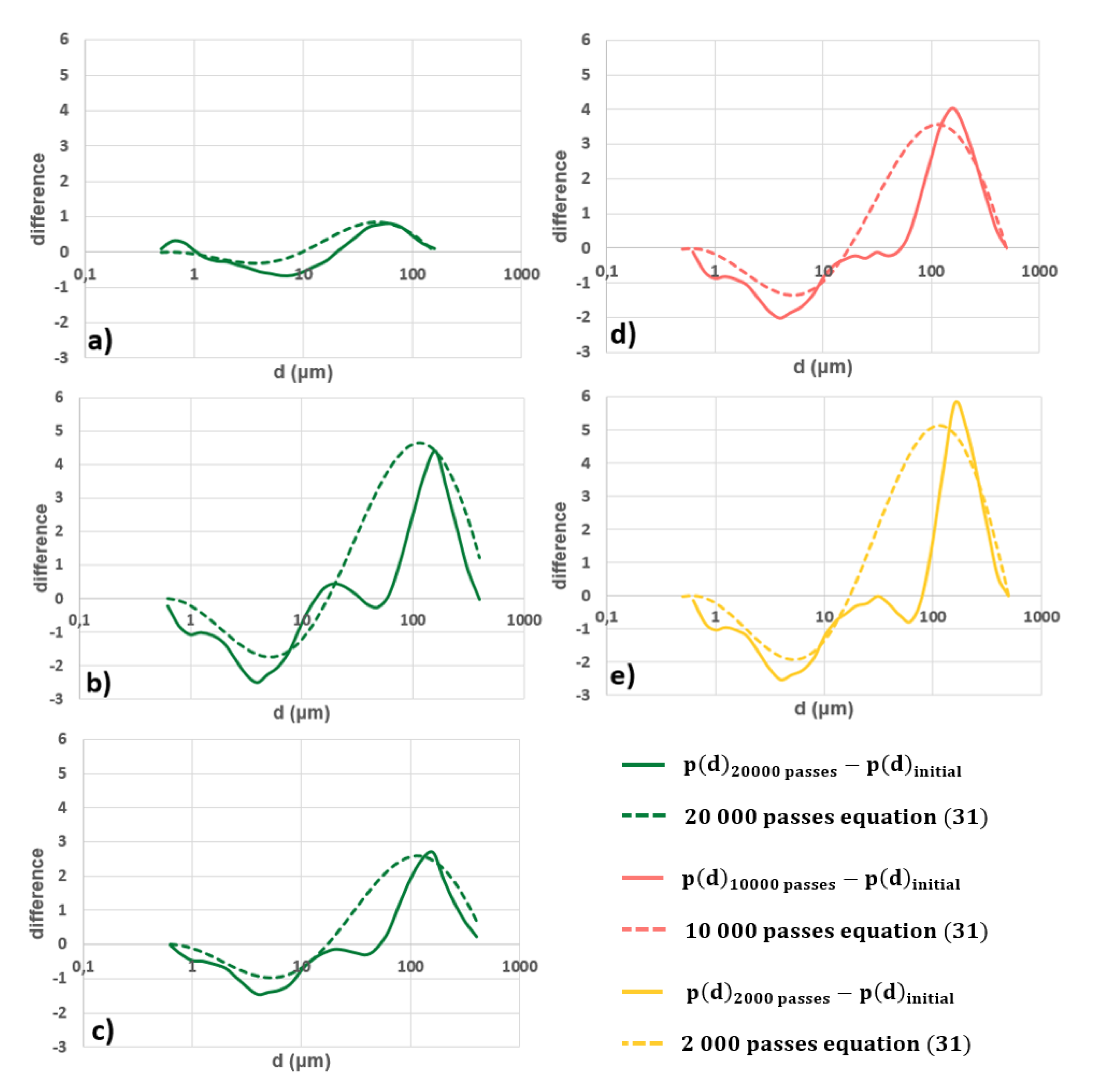
  • The g N function was determined from the curves in Figure A1c–e. Assuming that fsoil = 1, the value of g N corresponded to the amplitude A of Equation (26). Then, g N was determined by trial-and-error in order to minimize the average weighted deviation between experimental and theoretical curves. The weighted deviation was defined by:
    w e i g h t e d   d e v i a t i o n = | e x p e r i m e n t a l   v a l u e × ( e x p e r i m e n t a l   v a l u e t h e o r e t i c a l   v a l u e ) |
    A weighted deviation criterion was chosen in order to minimize the difference between experimental and theoretical curves for the amplitude peaks, which were the most important parts of the curve to model. According to that, it appeared that the best approximation for the function g N was a second-degree function:
    g N ( N ) = 9.72 × 10 10 N 2 4.92 × 10 5   N + 1.09
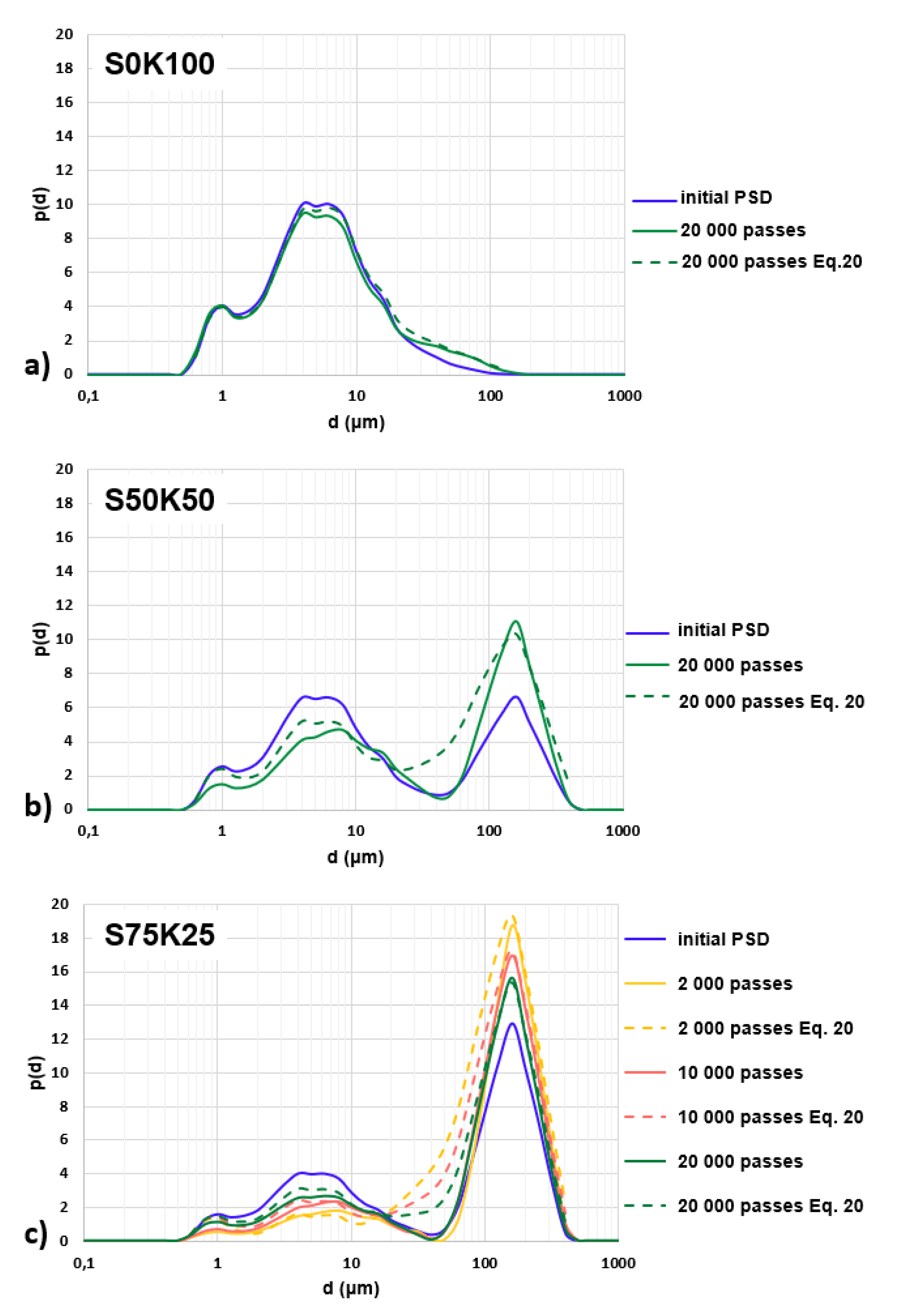
  • The fsoil function was determined using the curves in Figure A1a–c. These three curves corresponded to the case where g N (N = 20,000) = 0.49. The amplitude of the difference between 20,000 passes and initial soil was low for S0K100 (clay), medium for S75K25 and high for S50K50. Thus, it was considered that this amplitude depended on the product of the percentage of clay by the percentage of sand in the soil ( % c l a y × % s a n d ). According to this definition and based on the particle size distributions of the three soils, S0K100 had 20% clay and 7% sand ( % c l a y × % s a n d = 140 ), S50K50 had 13% clay and 36,6% sand ( % c l a y × % s a n d = 475.8 ) and S75K25 had 6,7% clay and 64% sand ( % c l a y × % s a n d = 428.8 ). The amplitude function of Equation (26) to approximate the curves in Figure A1a–c was therefore:
    A ( N = 20,000 ) = f N ( % c l a y × % s a n d ) × g N ( N = 20,000 ) = f N ( % c l a y × % s a n d ) × 0.49
As with the estimation of the g N function, the fsoil function was assessed by trial-and-error to minimize the weighted deviation (Equation (28)). The best approximation for fsoil was:
f s o i l ( % c l a y × % s a n d ) = 0.111 × e [ 0.004 ( % c l a y × % s a n d ) ]
Finally, the function for modelling the difference between the particle size distribution of the loose particles and the initial soil was defined by:
d i f f e r e n c e = 0.111 × e [ 0.004 ( % c l a y × % s a n d ) ] 0.49 × ( 9.72 × 10 10 N 2 4.92 × 10 5   N + 1.09 ) × ln ( d d m i n ) × s i n [ 2 π ln ( d m a x d m i n ) × ln ( d d m i n ) + π ]
The comparisons between the model estimates and the experimental results were shown in Figure A1. Relatively good agreements were found.

References

  1. Pouliot, G.; Simon, H.; Bhave, P.; Tong, D.; Mobley, D.; Pace, T.; Pierce, T. Assessing the anthropogenic fugitive dust emission inventory and temporal allocation using an updated specification of particulate matter. Air Pollut. Model. Its Appl. 2012, XXI, 585–589. [Google Scholar]
  2. Serpell, A.; Kort, J.; Vera, S. Awareness, actions, drivers and barriers of sustainable construction in Chile. Technol. Econ. Dev. Econ. 2012, 19, 272–288. [Google Scholar] [CrossRef] [Green Version]
  3. Pope, C.A.; Dockery, D.W. Health effects of fine particulate air pollution: Lines that connect. J. Air Waste Manag. Assoc. 2006, 56, 709–742. [Google Scholar] [CrossRef]
  4. Mohapatra, K.; Biswal, S.K. Effect of Particulate Matter on plants, climate, ecosystem and human health. Int. J. Adv. Technol. Eng. Sci. 2014, 2, 118–129. [Google Scholar]
  5. Moosmüller, H.; Varma, R.; Arnot, W.P.; Kuhns, H.D.; Etyemezian, V.; Gillies, J.A. Scattering cross-section emission factors for visibility and radiative transfer applications: Military vehicles traveling on unpaved roads. J. Air Waste Manag. Assoc. 2005, 55, 1743–1750. [Google Scholar] [CrossRef] [PubMed] [Green Version]
  6. Baddock, M.C.; Strong, C.L.; Leys, J.F.; Heidenreich, S.K.; Tews, E.K.; McTainsh, G.H. A visibility and total suspended dust relationship. Atmos. Environ. 2014, 89, 329–336. [Google Scholar] [CrossRef] [Green Version]
  7. Ashley, W.S.; Strader, S.; Dziubla, D.C.; Haberlie, A. Driving blind: Weather-related vision hazards and fatal motor vehicle crashes. Bull. Am. Meteorol. Soc. 2015, 96, 755–778. [Google Scholar] [CrossRef]
  8. Call, D.A.; Wilson, C.S.; Shourd, K.N. Hazardous weather conditions and multiple-vehicle chain-reaction crashes in the United States. Meteorol. Appl. 2018, 25, 466–471. [Google Scholar] [CrossRef] [Green Version]
  9. Gambatese, J.A.; James, D.E. Dust suppression using truck-mounted water spray system. J. Constr. Eng. Manag. 2001, 127, 53–59. [Google Scholar] [CrossRef]
  10. U.S. Environmental Protection Agency. Compilation of Air Pollutant Emission Factors, AP-42 5th ed.; Office of Air Quality Planning and Standards, Research Triangle Park: North Carolina, NC, USA, 1995.
  11. Gillies, J.A.; Etyemezian, V.; Kuhns, H.; Nikolic, D.; Gillette, D.A. Effect of vehicle characteristics on unpaved road dust emissions. Atmos. Environ. 2005, 39, 2341–2347. [Google Scholar] [CrossRef]
  12. Muleski, G.E.; Cowherd, C.; Kinsey, J.S. Particulate emissions from construction activities. J. Air Waste Manag. Assoc. 2005, 55, 772–783. [Google Scholar] [CrossRef] [PubMed] [Green Version]
  13. Etyemezian, V.; Kuhns, H.; Gillies, J.; Green, M.; Pitchford, M.; Watson, J. Vehicle-based road dust emission measurement: III—Effect of speed, traffic volume, location, and season on PM10 road dust emissions in the Treasure Valley, ID. Atmos. Environ. 2003, 37, 4583–4593. [Google Scholar] [CrossRef]
  14. Kuhns, H.; Gillies, J.; Etyemezian, V.; Nikolich, G.; King, J.; Zhu, D.; Uppapalli, S.; Engelbrecht, J.; Kohl, S. Effect of Soil Type and Momentum on Unpaved Road Particulate Matter Emissions from Wheeled and Tracked Vehicles. Aerosol Sci. Technol. 2010, 44, 187–196. [Google Scholar] [CrossRef]
  15. Bagnold, R.A. The transport of sand by wind. Geogr. J. 1937, 89, 409–438. [Google Scholar] [CrossRef]
  16. Greeley, R.; Iversen, J.D. Wind as a Geologic Process on Earth, Mars, Venus and Titan; Cambridge University Press: New York, NY, USA, 1985. [Google Scholar]
  17. Shao, Y.; Lu, H. A simple expression for wind erosion threshold friction velocity. J. Geophys. Res. 2000, 105, 22437–22443. [Google Scholar] [CrossRef]
  18. Nicholson, K.W.; Branson, J.R.; Geiss, P.; Cannel, R.J. The effects of vehicle activity on particle resuspension. J. Aerosol Sci. 1989, 20, 1425–1428. [Google Scholar] [CrossRef]
  19. Klose, M.; Shao, Y. Stochastic parameterization of dust emission and application to convective atmospheric conditions. Atmos. Chem. Phys. 2012, 12, 7309–7320. [Google Scholar] [CrossRef] [Green Version]
  20. Karafiath, L.L.; Nowatzki, E.A. Soil Mechanics for Off-Road Vehicle Engineering; Series on Rock and Soil Mechanics; Trans Tech Publications: Clausthal, Germany, 1978. [Google Scholar]
  21. Shao, Y. Physics and Modelling of Wind Erosion, 2nd ed.; Springer: Berlin, Germany, 2008. [Google Scholar]
  22. Klose, M.; Shao, Y.; Li, X.L.; Zhang, H.S.; Ishizuka, M.; Mikami, M.; Leys, J.F. Further development of a parameterization for convective turbulent dust emission and evaluation based on field observations. J. Geophys. Res. Atmos. 2014, 119, 10441–10457. [Google Scholar] [CrossRef]
  23. Li, X.L.; Klose, M.; Shao, Y.; Zhang, H.S. Convective Turbulent Dust Emission (CTDE) observed over Horqin Sandy Land area and validation of a CTDE scheme. J. Geophys. Res. Atmos. 2014, 119, 9980–9992. [Google Scholar] [CrossRef]
  24. Klose, M. Convective Turbulent Dust Emission: Process, Parametrization and Relevance in the Earth System. Ph.D. Thesis, University of Cologne, Cologne, Germany, 2014. [Google Scholar]
  25. ISO 13317-1:2001—Determination of Particle Size Distribution by Gravitational Liquid Sedimentation Methods—Part 1: General Principles and Guidelines; International Organization of Standardization: Geneva, Switzerland, 2001.
  26. ISO 2591-1:1988—Test Sieving—Part 1: Methods Using Test Sieves of Woven Wire Cloth and Perforated Metal Plate; International Organization of Standardization: Geneva, Switzerland, 1988.
  27. ISO 13320:2020—Particle Analysis—Laser Diffraction Methods; International Organization of Standardization: Geneva, Switzerland, 2020.
  28. Sediki, O. Étude des Mécanismes D’instabilité et D’envol des Particules en Lien avec L’hydratation des Sols Fins. Ph.D. Thesis, Université de Lorraine, Lorraine, France, 2018. (In French). [Google Scholar]
  29. Zimon, A.D. Adhesion of Dust and Powder; Consultants Bureau: New York, NY, USA, 1982. [Google Scholar]
  30. Corn, M. The adhesion of solid particles to solid surfaces, II. J. Air Pollut. Control Assoc. 1961, 11, 566–584. [Google Scholar] [CrossRef]
  31. Braaten, D.A.; Paw, U.K.T.; Shaw, R.H. Particle resuspension in a turbulent boundary layer—Observed and modelled. J. Aerosol Sci. 1990, 21, 613–628. [Google Scholar] [CrossRef]
  32. Biasi, L.; de los Reyes, A.; Reeks, M.W.; de Santi, G.F. Use of a simple model for the interpretation of experimental data on particle resuspension in turbulent flows. J. Aerosol Sci. 2001, 32, 1175–1200. [Google Scholar] [CrossRef]
  33. Orszag, S.A. Numerical methods for the simulation of turbulence. Phys. Fluids 1969, 12, II-250–II-257. [Google Scholar] [CrossRef]
  34. Berera, A.; Ho, R.D.J.G. Chaotic properties of a turbulent isotropic fluid. Phys. Rev. Lett. 2018, 120, 024101. [Google Scholar] [CrossRef] [Green Version]
  35. Rodriguez, S. Overview of fluid dynamics and turbulence. In Applied Computational Fluid Dynamics and Turbulence Modeling; Springer: Cham, Germany, 2019. [Google Scholar]
  36. Rohatgi, V.K. An Introduction to Probability Theory and Mathematical Statistics; Wiley Series in Probability and Statistics: New York, NY, USA, 1976. [Google Scholar] [CrossRef]
  37. Sediki, O.; Razakamanantsoa, A.R.; Hattab, M.; Le Borgne, T.; Fleureau, J.M.; Gotteland, P. Degradability of unpaved roads submitted to traffic and environmental solicitations: Laboratory scale. In Proceedings of the TC106 Conferences in Unsaturated Soils—7th International Conference of Unsaturated Soils, Hong Kong, China, 3–5 August 2018. [Google Scholar]
  38. Le Vern, M.; Sediki, O.; Razakamanantsoa, A.R.; Murzyn, F.; Larrarte, F. Experimental study of particle lift initiation on roller compacted sand-clay mixtures. Environ. Geotech. 2020, in press. [Google Scholar] [CrossRef]
  39. GTR. Guide Français Pour la « Réalisation des Remblais et des Couches de Forme», 2nd ed.; IFSTTAR-CEREMA; French Ministry of Ecology, Sustainable Development and Energy: Paris, France, 2000. (In French) [Google Scholar]
  40. Proctor, R.R. Fundamental principles of soil compaction. Eng. New Rec. 1933, 119, 245–248. [Google Scholar]
  41. Antille, D.L.; Bennett, J.M.; Jensen, T.A. Soil compaction and controlled traffic considerations in Australian cotton-farming systems. Crop Pasture Sci. 2016, 61, 1–28. [Google Scholar] [CrossRef]
  42. CATERPILLAR. Caterpillar Performance Handbook Edition 44: ARTICULATED TRUCK, Technical Paper. 2014. Available online: https://www.hawthornecat.com/sites/default/files/content/download/pdfs/Articulated_Trucks_CPH_v1.1_03.13.14.pdf (accessed on 3 December 2019).
  43. Midwest Research Institute. Improvement of Specific Emission Factors (BACM Project No. 1); Midwest Research Institute: Kansas City, MO, USA, March 1996. [Google Scholar]
  44. Djenedi, L.; Talluru, K.M.; Antonia, R.A. A velocity defect chart method for estimating the friction velocity in turbulent boundary layers. Fluid Dyn. Res. 2019, 51. [Google Scholar] [CrossRef]
  45. Schlichting, H. Boundary Layer Theory, 7th ed.; McGraw-Hill Book Comp.: New York, NY, USA, 1979. [Google Scholar]
  46. U.S. Department of Agriculture. Soil Survey Manual. In Soil Science Division Staff, Agricultural Handbook No. 18; Government Printing Office: Washington, DC, USA, March 2017. [Google Scholar]
  47. Etyemezian, V.; Kuhns, H.; Gillies, J.; Green, M.; Pitchford, M.; Watson, J. Vehicle-based road dust emission measurement: I—Methods and calibration. Atmos. Environ. 2003, 37, 4559–4571. [Google Scholar] [CrossRef]
  48. Organiscak, J.A.; Reed, W.R. Characteristics of fugitive dust generated from unpaved mine haulage roads. Int. J. Surf. Min. Reclam. Environ. 2004, 18, 236–252. [Google Scholar] [CrossRef]
  49. Reed, W.R.; Organiscak, J.A. Haul Road Dust Control: Fugitive dust characteristics from surface mine haul roads and methods of control. Coal Age 2007, 112, 34–37. [Google Scholar]
Figure 1. Log-normal distributions of cohesive forces fi for particles of 1 μm, 2 μm, 3.5 μm, 7.5 μm and 20 μm diameter, according to Equation (7).
Atmosphere 11 00369 g001
Figure 2. Laboratory roller compactor. (a) Schematic layout; (b) side view; (c) front view.
Atmosphere 11 00369 g002
Figure 3. (a) Side view of the VECTRA traffic simulator; (b) Front view of the schematic layout; (c) and (d) tires used in this study.
Atmosphere 11 00369 g003
Figure 4. Wind tunnel facility and zoom on the soil sample. Green crosses represent the velocity gradient measuring points with their Cartesian coordinates (x,y,z). Distances are in m.
Atmosphere 11 00369 g004
Figure 5. Evolution of soil surface degradation as a function of the number of wheel passes.
Atmosphere 11 00369 g005
Figure 6. Particle size distributions of loose particles and initial soils for sample (a) S0K100, (b) S50K50 and (c) S75K25.
Atmosphere 11 00369 g006
Figure 7. Particle size distributions measured (solid lines) and modeled (Equation (20), dashed lines) for sample (a) S0K100, (b) S50K50 and (c) S75K25.
Atmosphere 11 00369 g007
Figure 8. Example, for sample IV at a velocity of 8 m/s, of the process of determining p(τ). (a) Velocity fluctuations above the soil surface; (b) PDF of u′, at the measuring point designated by the cross, with determination of the parameters μ and σ from Equation (21); (c) PDF of τ determined using Equation (11).
Atmosphere 11 00369 g008
Figure 9. PDF of τ for the position x = 0.27 m and for (a) U = 8 m/s and (b) U = 16 m/s. The dotted lines represent the average curves that have been chosen to be implemented in the dust emission model.
Atmosphere 11 00369 g009
Figure 10. Estimated PM10 emissions of the three soils for 100, 1000 and 10,000 wheel passes and for both flow velocities U∞ = 8 m/s and U∞ = 16 m/s.
Atmosphere 11 00369 g010
Table 1. Soil samples compaction and degradation conditions.
SampleSoilDry Density after Compaction (kg·m−3)Water Content during Compaction (%)Water Content during Traffic Degradation (%)Number of Wheel Passes (N)Tire Type a
Sample IS0K1001470.0028.2021.1220,000M
Sample IIS50K501801.0016.0012.9820,000M
Sample IIIS75K251873.0012.409.4520,000M
Sample IVS75K251873.0012.408.9510,000M
Sample VS75K251873.0012.409.3020,000C
a M: tire MITAS FL-08; C: tire CONTINENTAL IC 10 (Figure 3).
Table 2. Vertical meshing of velocity measurement points.
Height from the Surface (y in mm)Vertical Spacing between Two Measuring Points (mm)Number of Measuring Points
0 y 2 0.1021
2.2 y 3 0.205
3.5 y 5 0.504
6 y 10 1.005
12 y 20 2.005
30 y 50 10.003
Table 3. Parameters of the degradation model (Equation (18)).
Soilc1c2c3c4c5Corresponding Equation
S0K100 5.69 × 10 2 3.23 × 10 3 1.24 × 10 5 4.86 × 10 1 4.20 × 10 2 (18-a)
S50K50 1.38 × 10 1 8.51 × 10 2 4.41 × 10 1 2.14 × 10 2 1.50 × 10 4 (18-b)
S75K25 1.11 × 10 1 8.40 × 10 3 1.26 × 10 4 2.09 × 10 1 1.58 × 10 4 (18-c)
Table 4. Parameters related to velocity profiles.
PositionU = 8 m/sU = 16 m/s
Hu* (m/s)δvs (µm)Hu* (m/s)δvs (µm)
Sample Ix = −0.03 m1.720.263001.230.51153
x = 0.05 m1.450.292691.230.44177
x = 0.15 m1.370.282781.300.58134
x = 0.27 m1.260.243251.260.53147
Sample IIIx = −0.03 m1.780.322441.390.54144
x = 0.05 m1.220.302601.520.62126
x = 0.15 m1.500.342291.330.66118
x = 0.27 m1.380.312521.350.62126
Sample IVx = −0.03 m1.700.322441.320.55142
x = 0.05 m2.180.721082.031.3757
x = 0.15 m1.710.272891.230.73107
x = 0.27 m1.240.213711.220.51153
Sample Vx = -0.03 m1.620.322441.730.65120
x = 0.05 m1.420.174591.160.42186
x = 0.15 m1.390.243251.230.62126
x = 0.27 m1.190.174591.160.45173
Table 5. Vehicle characteristics and dust emission factors for the study of Gillies et al. [11].
Vehicle TypeWeight (kg)Tire Width (m)EF (kg·vkt−1)EF (kg·m−2) b
Ut = 30 km·h−1Ut = 60 km·h−1
GMC C55005 2270.2450.0019 × Ut a0.00120.0023
M977 HEMTT17 7270.4000.0048 × Ut0.00180.0036
M923A2 (5-ton)14 3180.3550.0047 × Ut0.00200.0040
M1078 LMTV8 0600.3950.0018 × Ut0.00070.0014
a Ut: truck speed (km·h−1); b The emission factor expressed in mass per unit area is calculated by considering the wheels/road contact area along the truck journey (contact area = 2 × tire width × distance travelled).

