The Influence of Five Teleconnection Patterns on Wintertime Extratropical Cyclones over Northwest Pacific

Abstract

Extratropical cyclones (ETCs) over the Northwest Pacific are identified and tracked by applying an objective tracking algorithm to the 6-h time interval relative vorticity fields from the European Center for Medium-range Weather Forecasts (ECMWF) reanalysis data. A total of 2145 ETCs in the November–February winters for the period of 1979–2018 were identified. First, by comparing the ETC track densities in the two periods 1979–1998 and 1999–2018, a significant difference in ETC track density was detected over the Japan Sea, Japan, and North Pacific. Next, the influence of five teleconnection patterns, the El Niño-Southern Oscillation (ENSO), Western Pacific (WP), North Atlantic Oscillation (NAO), Pacific/North American (PNA), and Pacific Decadal Oscillation (PDO) on the ETC track density was investigated by using composite analysis and correlation analysis. WP, NAO, and PDO patterns contributed more to the interannual variability of ETC track density, and higher cyclone densities usually occur in the negative phase of these teleconnection patterns. In contrast, the effects of ENSO and PNA were relatively weak. Finally, a Poisson generalized linear regression model for the ETC counts with respect to the five teleconnection indices was also developed for the purpose of linking all the teleconnection patterns with ETC activities over Northwest Pacific; and the Bayesian model averaging (BMA) procedure was used for model selection in the statistical modeling. The influence of the five teleconnection patterns on ETC track density was also verified in the regression model. The predicted winter ETC counts agreed well with the historical records during 1979–2018 over the Northwest Pacific.

1. Introduction

Extratropical cyclones (ETCs), also called wave cyclones or midlatitude cyclones, are baroclinic low pressure vortices over mid and high latitudes of the two hemispheres. They play an important role in the atmospheric general circulation by transferring heat, moisture, and kinetic energy between the tropics and Polar Regions [1,2]. In addition, ETCs are important synoptic systems that affect weather variability over a wide area of mid and high latitudes. Driven by baroclinic instability, ETCs with frontal systems may cause extreme weather. The passage of ETC is usually associated with strong winds, excessive precipitation, and sharp temperature changes resulting in economic and life losses [3,4,5].

The Northwest Pacific is one main region with strong wind storms in the Northern Hemisphere [6]. It is known as a storm-track region, which is defined as a region of frequent pathways of extratropical cyclones [7]. ETCs have significant weather impact here. A large proportion of precipitation extremes is found to be associated with ETCs over the South China Sea and near Japan [8]. Tu et al. [9] found that the explosive development of ETCs was related to sandstorms in north China, and that the explosive cyclones also had a close relationship with snowstorm over northeast China [10]. There is evidence of the changes in ETC activities in the Northern Hemisphere. McCabe et al. [11] found that cyclone frequency increased in high-latitude and decreased in midlatitude, and cyclone intensity increased in both midlatitude and high-latitude. During 1958–1999, cyclone intensity increased in the western Pacific and Atlantic, whereas in the eastern Pacific and continental North America, the cyclone activity showed an opposite trend [12]. Favre et al. [13] also found that cyclones over northeastern Pacific had been intensifying, with their pathways shifting southward since the mid-1970s.

As we know, atmospheric and oceanic teleconnection patterns have a deep influence on the global climate system. The interannual variability of cyclone tracks may be attributed to these teleconnection patterns. In this study, three atmospheric teleconnections (North Atlantic Oscillation, West Pacific, and Pacific-North American) and two oceanic teleconnections (El Niño-Southern Oscillation and Pacific Decadal Oscillation) were considered. The El Niño-Southern Oscillation (ENSO) is one main oceanic teleconnection pattern with two opposite phases named El Niño and La Niña, respectively [14]. El Niño (La Niña) refers to a periodic warming (cooling) in ocean surface temperatures in the central and east-central equatorial Pacific. Eichler et al. [15] proposed that ENSO could affect cyclone activity over the North Pacific. In El Niño (EN) years, cyclone tracks are prone to move equatorward, while in La Niña (LN) years, there is a poleward shift in cyclone tracks. For the North Atlantic Oscillation (NAO), it has been reported that there exists a significant influence on storm frequency over the Atlantic as well as cyclonic activity over the North Pacific [16]. When the NAO is in positive (negative) phase, the pattern reflects below (above) normal heights and pressure across the high latitudes of the North Atlantic and above (below) normal heights and pressure over the central North Atlantic. The Pacific-North American (PNA) pattern is associated with strong fluctuations in the strength and location of the East Asian jet stream [17], and this pattern was found to be associated with the frequency of cyclones in the eastern Pacific [12]. Pacific Decadal Oscillation (PDO) is associated with monthly sea surface temperature (SST) anomalies in the North Pacific; in its positive (negative) phase, the PDO consists of negative (positive) SST anomalies in the central and western North Pacific. The Canadian cyclone activity is related to the NAO, PDO, and ENSO, in general, the cyclone activity is most closely related to NAO [18]. The West Pacific (WP) pattern consists of a north–south dipole of anomalies; during winter, both phases of WP reflect significant zonal and meridional changes in the location and intensity of the entrance region of the Pacific jet steam [19]. Li et al. [20] showed that PDO, PNA, and WP teleconnection patterns were closely related to the variation of the North Pacific storm track in winter.

The influence of teleconnection patterns on climate anomalies might be revealed by composite maps during the opposite phases of these teleconnections [21]. Additionally, the relationship between climate variables and cyclonic activity could be modeled by the generalized linear models (GLM). For cyclone activities, Villarini et al. [22] modeled the relationship between annual counts of tropical storms and climate indices during 1878–2008. In the process of statistical modeling, model uncertainty is an inevitable problem. Here, model uncertainty refers to the ambiguity associated with choosing a single model from a suite of similarly good models. Bayesian model averaging (BMA) is one commonly applied method for model selection in statistical modeling. Actually, the BMA method produces a weighted average of all model predictions, rather than choosing a single model [23]. In this way, the problem of model uncertainty could be effectively solved. Jagger et al. [24] analyzed the influence of some climate indices on U.S. hurricane counts, and examined the effectiveness of these climate indices for predicting hurricane counts by using the BMA procedure.

In this study, we first assessed the change in ETC track density for the periods of 1979–2018 over the Northwest Pacific. The second objective was to study the influence of the five teleconnection patterns of ENSO, PDO, PNA, NAO, and WP on ETC tracks. Finally, the BMA procedure was applied to produce a consensus cyclone prediction model. The rest of this work is organized as follows. Section 2 presents the data and methodology used in this study. Section 3.1 shows the climatology of ETC density over the Northwest Pacific and change in cyclone track density. The association between teleconnection patterns and cyclone occurrences are presented in Section 3.2. The statistical modeling of ETC counts based on Poisson regression and the BMA method are given in Section 3.3. Finally, Section 4 presents a brief discussion and some conclusions.

2. Data and Methodology

2.1. Data

The study area was bounded within the region 20° N–60° N and 90° E–120° W over the Northwest Pacific, while the period was the November–February winter seasons starting from 1979 to 2018. The relative vorticity fields at 850 hPa level used in this study for ETC identification and tracking were derived from the European Center for Medium range Weather Forecasts (ECMWF) Interim (ERA-I) reanalysis data (20° N–80 °N, 60° E–120° W), with a 0.75° × 0.75° horizontal resolution and 6-h time interval. The datasets were accessed from NCAR’s Research Data Archive (https://rda.ucar.edu/).

The monthly time series for the atmospheric teleconnection indices WP, PNA, and NAO were provided by the National Oceanic and Atmospheric Administration Climate Prediction Center (https://www.cpc.ncep.noaa.gov/data/teledoc/telecontents.shtml). The Niño-3.4 index was used to reflect ENSO, and the monthly time series ENSO and PDO indices were provided by the National Center for Atmospheric Research’s Climate and Global Dynamics Division (https://climatedataguide.ucar.edu/climate-data).

2.2. Extratropical Cyclone (ETC) Identification and Tracking

In this study, the objective algorithm presented in [25] was used to identify and track ETCs based on the relative vorticity fields at the 850 hPa level. The algorithm includes two steps: the first step is to identify the centers of the cyclones, and the second step is to combine these centers into a track. This identification and tracking algorithm performs well in comparison with other techniques using 1000 hPa geopotential height or minimum sea level pressure [25]. Specifically, before identifying cyclone centers, the means filtering algorithm is used to smooth the relative vorticity fields. We chose the same threshold 3 × 10⁻⁵ s⁻¹ as in [25]; only the grid points exceeding the threshold were retained. Thus, the cyclones were defined as the areas composed of neighboring grid points of values exceeding the 3 × 10⁻⁵ s⁻¹ threshold. Next, all the potential cyclone paths were identified by linking the cyclone centers at consecutive time steps and selecting the most probable track based on the minimization of a cost function. The cost function was based on the average differences of relative vorticity between consecutive track points, weighted by their distance. “An effective area” for each cyclone was also identified based on different physical diagnostics such as the minimum sea level pressure and the maximum wind speed.

The cyclones tracked by the above method include all cyclones, while only ETCs with a lifetime of at least 24 h were studied. This consideration gets rid of local warm season thermal lows [26]. Cyclone processes are classified as motionless cyclones (moving within five longitude degrees in distance) and mobile cyclones (else). Motionless cyclones are removed when eliminating local warm season thermal lows [27]. Additionally, there are a few false paths in which cyclones move upstream/westward over five longitude degrees in distance during their lifespan (occupying about 5% of all tracks). The frontal cyclones move along the direction of tropospheric airflow [28]; however, airflow in the troposphere basically moves from west to east. It is possible that some tropical cyclones moving westward from the Northwest Pacific to the East-Asian continent may be tracked, so the spurious paths of cyclones moving westward over five longitude degrees were also eliminated. Moreover, only ETCs originating in the region 20°–60° N, 90° E–180° E and ETC tracks extending to the 140° W meridian were considered in this study. In this study, we took the number of cyclones in each grid as the cyclone density. Considering the range of our study area, a grid size of 4° × 5° was applied to discretize the study area for the purpose of showing the spatial pattern of the ETC track density. For each grid, only the cyclone that moved across the meridian line within ±10° latitude from the grid center was counted [29].

2.3. Composite Analysis and Correlation Analysis

In this study, the influence of the five teleconnection patterns, ENSO, PDO, PNA, NAO, and WP on ETC track density was evaluated through composite analysis and correlation analysis, respectively. Composite analysis of cyclones has been employed for many purposes using different methodologies. It helps to effectively characterize cyclogenesis [30], analyze explosively deepening cyclones [31,32], and rapidly decaying cyclones [33,34,35] as well as the tropical to extratropical cyclone transitions in the Atlantic [36]. The composite analysis could provide a general idea of how the cyclones respond to the teleconnection patterns. The positive and negative phases were defined as when the teleconnection index values fell in the upper and lower 25% of the indices’ distribution, respectively [21]. Correlation analysis was also used to quantify the association between teleconnection indices and ETC track densities in each grid. Since ETC track densities were computed from the discrete ETC counts, the Kendall rank correlation was adopted in the correlation analysis.

2.4. Poisson Regression Model of the ETC Count

For the ETC counts data, we assumed that the observations in each winter over the Northwest Pacific, denoted as $n$, followed a discrete Poisson distribution:

$$p\left(n\right)=\frac{e^{-\lambda }{\lambda }^n}{n!},$$

(1)

Here, λ is the only model parameter representing the expectation of the Poisson distribution, which is a non-negative random variable. Poisson regression is a form of regression model, in which the response variable is in the form of count data. The logarithm of the model parameter λ is regressed onto the covariates—that is,

$$\log \left(\lambda \right)={\beta }_0+{\beta }_1{x}_1+\cdots +{\beta }_k{x}_k+\epsilon ,$$

(2)

There are $k$ covariates (in this case, teleconnection pattern index) indicated by $x_i$ (i= 1,…k) and $k+1$ coefficients ${\beta }_j$(j = 1,…k + 1). Additionally, with the $k$ covariates, there is theoretically a total of $m=2^k$ potential regression models with different combinations of covariates as inputs. The vector ε is a set of independent and identically distributed residuals.

Poisson regression is nonlinear in the regression function, but linear in regression structure. The model coefficients could be determined by the maximum likelihood estimation method. With the Poisson regression model, future ETC counts depend on these covariate values following a Poisson distribution with a model parameter λ, and consequently a probabilistic prediction could be obtained. To improve the model fitness, model selection is a key step in statistical modeling. This selection could be implemented according to the criteria such as Akaike information criterion (AIC) [37], Bayesian Information criterion (BIC), or a cross-validation score. These model selection methods attempt to find a single best model from all potential models with different combinations of covariates. Bayesian model averaging (BMA) is an alternative model selection procedure; it keeps all potential models, but assigns a probability based on likelihood for the data that come from the potential model. Then, a consensus model, representing a weighted average of all models, is used to make predictions. More details on the BMA method can be found in [24]. In this study, we used the BIC approximation for the posterior model probabilities [38]. The BMA procedure was carried out using the BMA package in the R computing environment [39,40].

3. Results

Before conducting the composite and correlation analyses, the oceanic and atmospheric background states were examined for the purpose of better understanding the climatology of ETCs over the Northwest Pacific. Figure 1 shows the wintertime sea surface temperature (SST) distribution and the climatological zonal wind at 300 hPa pressure level. Figure 1a shows that in the Kuroshio–Oyashio Extension, there was an obvious SST meridional gradient, which is associated with an intense westerly jet stream in the upper troposphere through the thermal wind balance (Figure 1b). Many of the weather systems that developed in East Asia are along this jet stream eastward [41]. These two oceanic and atmospheric conditions contribute to the formation and development of ETCs over the Northwest Pacific. In addition, there are other processes that also affect cyclones such as latent heat release and downstream developments [2].

3.1. Change of ETC Density

In order to identify the preferential tracks of ETCs over the Northwest Pacific in different periods, the ETC track density is presented first. The whole study period was divided into two periods 1979–1998 and 1999–2018, and the change in ETC density over the study area was compared in this two periods. Figure 2 shows the track density of ETCs over the Northwest Pacific. From Figure 2, we found that a higher cyclone track density occurred in the region zonally ranging from northern Japan, Hokkaido Island to the North Pacific in the earlier period. In the later period, the area of higher cyclone track density was larger; in eastern Japan and the North Pacific, the ETC density was higher than that in the earlier period.

Generally, ETC densities in the two periods were almost similar, and this difference could be more clearly identified by subtracting the ETC density in the later period by that in the earlier period. Figure 2c shows the change of ETC track density between the earlier period (1979–1998) and later period (1999–2018). ETC density increased in the Japan Sea, Japan, and the North Pacific, but decreased over the south of the Kamchatka Peninsula; however, the change was not statistically significant.

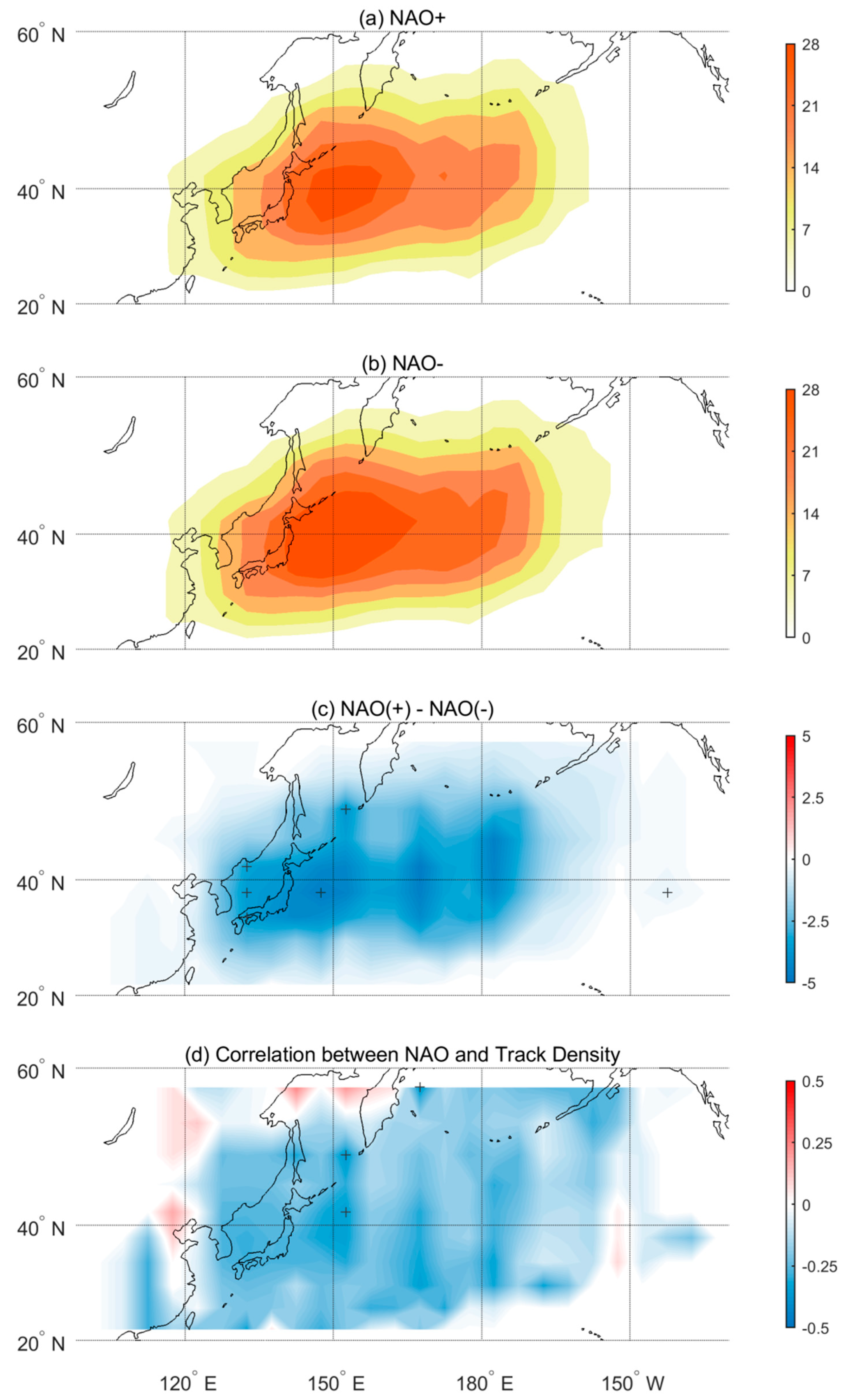
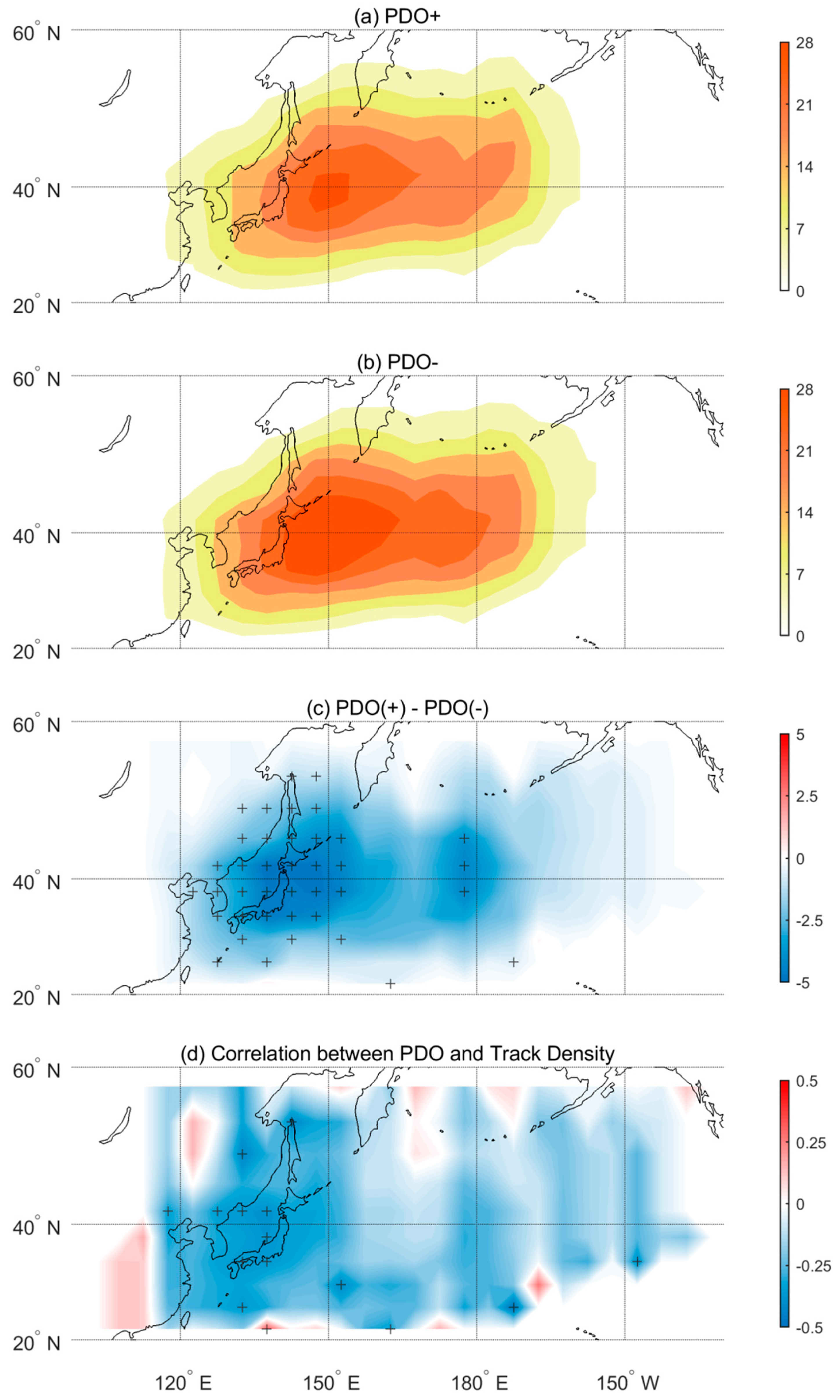
3.2. Influence of Teleconnection Patterns on ETC Track Density

Composites of the ETC densities in different phases of teleconnection patterns are presented to investigate their influences on the spatial patterns of ETC tracks. Figure 3a,b shows the composites of ETC densities in the El Niño and La Niña years in the winter from 1979 to 2018. In El Niño years, higher cyclone density was located over the Japan Sea, Japan, the south of the Okhotsk Sea, and the Northwest Pacific. In La Niña years, the spatial pattern of ETC density was similar to that in the El Niño years. Furthermore, the delicate difference between the ETC densities in the El Niño and La Niña years is shown in Figure 3c. We found that the difference in ETC density was not statistically significant. This means that the influence of ENSO on ETC density over Northwest Pacific is weak. Additionally, the correlation coefficients between the ENSO index and ETC density shown in Figure 3d partly verifies the above result.

ETC track density in different WP phases is shown in Figure 4a,b. In the negative phase of WP, ETC density was obviously higher than that in the positive phase. Grids with higher ETC density were located over the east of Japan, extending to the northwest Pacific. The difference of ETC density between WP(+) and WP(−) is shown in Figure 4c. A statistically significant difference was detected over Sakhalin and some areas of the North Pacific. Figure 4d shows the correlations between the WP index and ETC density, and significant negative correlations were detected in the majority of grids in the study area. Both the composite analysis and correlation analysis verified the significant influence of WP on ETC activities over the Northwest Pacific.

Figure 5 shows the composites of ETC density in the positive and negative phases of PNA. In general, ETC density in the positive phase was higher over eastern Japan and North Pacific than that in the negative phase (Figure 5a,b). The difference of ETC density between these two phases could be detected where there was a higher cyclones density over eastern Japan in the positive phase and over the Korean Peninsula and Japan Sea in the negative phase (Figure 5c). The difference was not statistically significant for most grids. Similar spatial patterns of correlations between the PNA index and ETC track density are presented in Figure 5d.

ETC track density in the different NAO phases is shown in Figure 6a,b. We found that the spatial patterns of ETC density in the positive and negative phases of NAO were similar to those in the positive and negative phases of WP, respectively. ETC density in the negative phase was higher than that in the positive phase over the whole study area. The difference was only statistically significant in a few grids revealed by the t-test. The correlation analysis for NAO and ETC track density shown in Figure 6d showed the same situations. Finally, the spatial patterns of ETC density in different PDO phases are presented in Figure 7a,b. Obviously, ETC density in negative phase of PDO was higher than that in the positive phase. The grids with statistically significant differences were mainly located at the Korean Peninsula, extending to eastern Japan and the North Pacific (Figure 7c). This implies the significant influence of PDO on ETC activities over the Northwest Pacific. The significant negative correlations for the PDO index and ETC track density were widely distributed over Japan and the Japan Sea (Figure 7d).

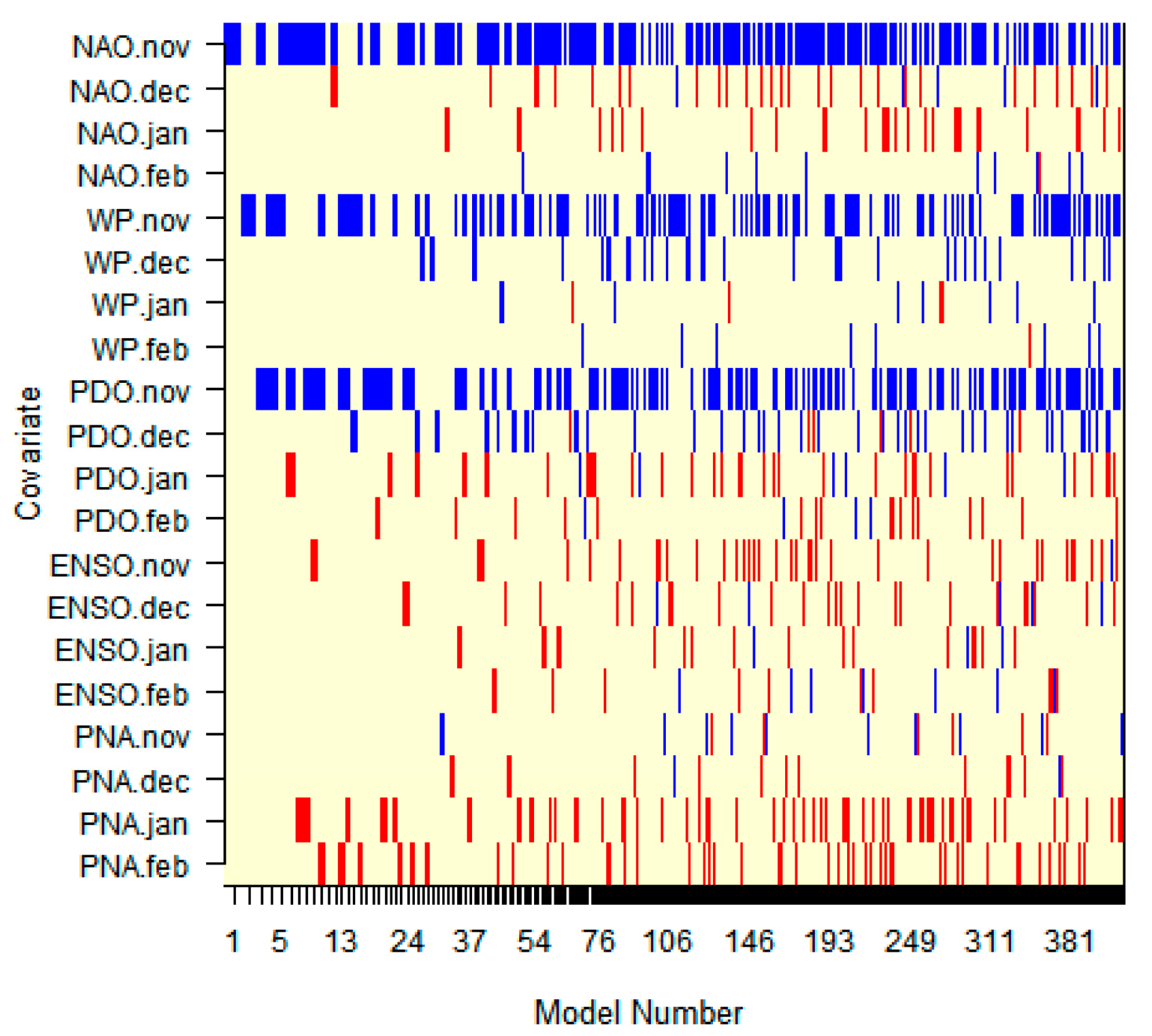
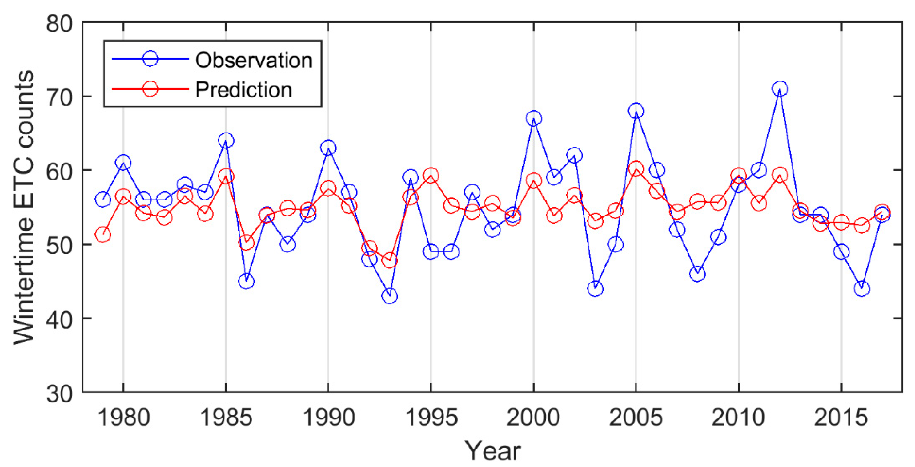
3.3. Statistical Modeling of ETC Counts

The Poisson regression model was used to analyze the association between cyclone counts and the above five teleconnection patterns. There were 434 models in total after the BMA model selection procedure. The models were ordered by BIC so that the first model had the lowest BIC value, the second model had the second lowest BIC, and so on. The top five models that had the smallest BIC are shown in

Table 1. Posterior statistics of the output from a BMA procedure. The P! = 0 is the posterior probability of the model parameter. The EV and SD are the expected value and standard deviation of the posterior parameters, respectively. The values under the model numbers are the regression coefficients with positive values indicating a positive relationship between the covariate and the probability of a extratropical cyclone.

	P! = 0	EV	SD	Model 1	Model 2	Model 3	Model 4	Model 5
Intercept	100	4.0020	0.0232	4.0102	4.0106	4.0000	3.9998	4.0119
NAO.nov	63.0	−0.0355	0.0353	−0.0528	─	−0.0504	─	−0.0407
NAO.dec	9.6	0.0030	0.0138	─	─	─	─	─
NAO.jan	6.9	0.0014	0.0080	─	─	─	─	─
NAO.feb	3.2	−0.0003	0.0046	─	─	─	─	─
WP.nov	43.6	−0.0192	0.0267	─	−0.0460	─	−0.0452	−0.0337
WP.dec	9.8	−0.0026	0.0109	─	─	─	─	─
WP.jan	3.7	−0.0002	0.0052	─	─	─	─	─
WP.feb	2.6	−0.0001	0.0036	─	─	─	─	─
PDO.nov	46.3	−0.0200	0.0276	─	─	−0.0312	−0.0331	─
PDO.dec	15.4	−0.0059	0.0239	─	─	─	─	─
PDO.jan	12.0	0.0059	0.0226	─	─	─	─	─
PDO.feb	6.1	0.0015	0.0114	─	─	─	─	─
PNA.nov	4.6	−0.0002	0.0062	─	─	─	─	─
PNA.dec	4.6	0.0008	0.0069	─	─	─	─	─
PNA.jan	18.7	0.0066	0.0172	─	─	─	─	─
PNA.feb	17.1	0.0055	0.0154	─	─	─	─	─
ENSO.nov	10.7	0.0064	0.0382	─	─	─	─	─
ENSO.dec	7.6	−0.0007	0.0343	─	─	─	─	─
ENSO.jan	5.4	0.0001	0.0152	─	─	─	─	─
ENSO.feb	4.9	−0.0001	0.0139	─	─	─	─	─
BIC				−109.73	−109.19	−108.93	−108.76	−108.47
Post prob				0.019	0.015	0.013	0.012	0.010

. The first column in the table is the intercept and covariates; the second column (P! = 0) is the posterior probability of the model parameter. For example, the covariate NAO in November has a probability of 63% of being included in a model. The column “EV” and “SD” represent the BMA posterior mean and standard, respectively. The following five columns show the parameter estimates for the best five models found, together with their BIC values and their posterior model probabilities. For instance, the covariate included in the most probable model (model 1) was November NAO.

All 434 models are shown in Figure 8. The model posterior probability decreased from left to right. The first model is in the left bar, which includes the November NAO covariate. The color bar is blue, which indicates that the probability of Northwest Pacific ETCs decreases with November NAO. The width of the bar is proportional to the posterior probability so the bars become narrow with increasing model number. A covariate that has a more consistent color bar is more important. The fewer the gaps, the more often the covariate is chosen in a model. These included November NAO, November WP, and November PDO. Time series generated by the regression model by the BMA for the ETC counts are shown in Figure 9. The red and blue lines represent the predicted and observed ETCs in winter over the Northwest Pacific, respectively. In addition, we used cross validation to compare the skill of BMA with the skill of other selection procedures. Both selection procedures involved the single best Poisson GLM, where best was defined as the model with the smallest BIC or the model with the smallest AIC [24]. For the BMA and selection procedures, we calculated the mean squared error (MSE), root mean squared error (RMSE), and mean absolute error (MAE) (

Table 2. Cross validation skill scores. The skill scores include MSE, RMSE, and MAE. Methods include BMA and the single best Poisson GLM. A smaller score refers to a procedure resulting in a more accurate prediction.

Method	MSE	RMSE	MAE
BMA	3.07	1.75	1.59
Smallest BIC	4.25	2.06	1.91
Smallest AIC	12.13	3.48	2.99

), where the smaller the indictors, the more accurate the result.

4. Summary and Discussion

In this study, wintertime ETCs over the Northwest Pacific in 1979–2018 were identified and tracked using an improved objective identification and tracking method. The objective method found cyclone locations based on 850 hPa relative vorticity fields. Non-significant change of wintertime ETC track density was detected during the past four decades over East Asia and Northwest Pacific. The influence of the five teleconnection patterns (ENSO, PNA, WP, NAO, and PDO) on ETC track density from 1979 to 2018 was investigated using composite analysis and correlation analysis.

In El Niño winters, ETC track density was lower than normal over the northeast of China to Japan. Eichler et al. [15] reported that ENSO has an impact on cyclone activity over the North Pacific. However, the association between ENSO and ETC activity variability over the Northwest Pacific revealed by composite analysis and correlation analysis in this study was not statistically significant.

The WP teleconnection pattern could be identified from the anomaly field of geopotential height existing throughout the year [42]. Strong positive or negative phases of WP pattern reflect pronounced zonal and meridional variations in the location and intensity of the entrance region of the East Asian jet steam (EAJS) [19]. In our study, WP teleconnection patterns were closely related to ETC track density. We found that there was a negative correlation between ETC density and WP. This means that wintertime ETC activity is less active in the positive phase of WP. Favorable conditions for cyclone development are strong dynamical forcing of the upper-level jet stream and large atmospheric baroclinicity [43]. In different phases of the WP pattern, the reason for the cyclones’ difference may be that the WP pattern is associated with the Pacific jet.

The PNA teleconnection pattern is one of the leading patterns of Northern Hemisphere midlatitude variability, which is also associated with strong fluctuations in the strength and location of the EAJS [17,42]. Li et al. [20] showed that the PDO, PNA, and WP teleconnection patterns that described the variation of the atmosphere–ocean system were closely related to the variation in the North Pacific storm track in winter. The interdecadal variations of the meridional position of storm track were basically consistent with the phase transitions of PNA and PDO, which may be important factors of the interdecadal anomalous variations of storm track. Wang et al. [18] found that cyclone activity in Canada was closely related to the PDO. However, in this study, the relationship between different phases of PDO and cyclone density was obvious, which is mainly because the baroclinicity in the negative phase of PDO tends to strengthen and shift poleward [44], while the relationship between the PNA teleconnection pattern and ETC track density was not obvious.

NAO not only affects the atmospheric circulation in the Atlantic, but also plays an important role in global large-scale atmospheric circulation [45,46,47,48]. The spring extratropical cyclones over the Yellow, Bohai, and East China Seas are correlated to NAO in the preceding winter (DJF) [16]. In this study, the influence of the NAO teleconnection pattern on ETC track density over the Japan Sea and Japan was also obvious, and the NAO may affect ETCs through the upper-level jet stream over Japan [16].

Regarding the relationship between teleconnection patterns and cyclone counts, the Poisson regression model was used. The BMA procedure that assigns a posterior probability to all models was applied for model selection. A consensus forecast could then be issued that represents a weighted average of forecasts from all potential models. The weights were simply the posterior probabilities assigned to each model [24]. For the BMA, the model posterior probabilities provide insight into the physical processes connecting the covariates to ETC activity. The covariate chosen most often was November NAO, followed by November PDO. The WP and NAO teleconnection indices almost showed a negative relationship, this indicates the chance of cyclone decreases with WP and NAO. However, this regression model has some limitations. For some extreme values (high/low ETC counts), it does not fit well. We will seek a more suitable model in further study in order to improve the fitting performance.

The study has only given insight into the relationship between the large-scale teleconnection patterns and the ETC number over the Northwest Pacific during the winter seasons. However, cyclone intensity was not included, and further exploration of the role of the teleconnection patterns on cyclone intensity will be the subject of our forthcoming research.

References

1. Zhang, Y.C.; Rossow, W.B. Estimating meridional energy transports by the atmospheric and oceanic general circulations using boundary fluxes. J. Clim. 1997, 10, 2358–2373. [Google Scholar] [CrossRef]
2. Chang, E.K.M.; Lee, S.Y.; Swanson, K.L. Storm track dynamics. J. Clim. 2002, 15, 2163–2183. [Google Scholar] [CrossRef] [Green Version]
3. Ulbrich, U.; Leckebusch, G.C.; Pinto, J.G. Extra-tropical cyclones in the present and future climate: A review. Theor. Appl. Climatol. 2009, 96, 117–131. [Google Scholar] [CrossRef] [Green Version]
4. Hawcroft, M.K.; Shaffrey, L.C.; Hodges, K.I.; Dacre, H.F. How much Northern Hemisphere precipitation is associated with extratropical cyclones? Geophys. Res. Lett. 2012, 39. [Google Scholar] [CrossRef] [Green Version]
5. Catto, J.L. Extratropical cyclone classification and its use in climate studies. Rev. Geophys. 2016, 54, 486–520. [Google Scholar] [CrossRef]
6. Iwao, K.; Inatsu, M.; Kimoto, M. Recent Changes in Explosively Developing Extratropical Cyclones over the Winter Northwestern Pacific. J. Clim. 2012, 25, 7282–7296. [Google Scholar] [CrossRef]
7. Whittaker, L.M.; Horn, L.H. Northern Hemisphere extratropical cyclone activity for 4 mid-season months. J. Climatol. 1984, 4, 297–310. [Google Scholar] [CrossRef]
8. Pfahl, S.; Wernli, H. Quantifying the Relevance of Cyclones for Precipitation Extremes. J. Clim. 2012, 25, 6770–6780. [Google Scholar] [CrossRef]
9. Tu, N.N.; Jiao, M.Y.; Zhao, L.N.; Zhu, W.J. Dynamical Characteristics for a Mongolia Cyclone Associated with Sand-Dust Storm in North China. J. Desert Res. 2007, 27, 520–527. [Google Scholar]
10. Lina, C.A.I.; Yingjiu, S.U.I.; Daqing, L.I.U.; Shuang, W.; Wei, L.I.U.; Tiankui, W. Analysis on an Unusual Snowstorm Event Caused by Explosive Cyclone. Acta Sci. Nat. Univ. Pekin. 2009, 45, 693–700. [Google Scholar]
11. McCabe, G.J.; Clark, M.P.; Serreze, M.C. Trends in Northern Hemisphere surface cyclone frequency and intensity. J. Clim. 2001, 14, 2763–2768. [Google Scholar] [CrossRef]
12. Gulev, S.K.; Zolina, O.; Grigoriev, S. Extratropical cyclone variability in the Northern Hemisphere winter from the NCEP/NCAR reanalysis data. Clim. Dyn. 2001, 17, 795–809. [Google Scholar] [CrossRef]
13. Favre, A.; Gershunov, A. Extra-tropical cyclonic/anticyclonic activity in North-Eastern Pacific and air temperature extremes in Western North America. Clim. Dyn. 2006, 26, 617–629. [Google Scholar] [CrossRef]
14. Chen, S.F.; Yu, B.; Chen, W.; Wu, R.G. A Review of Atmosphere-Ocean Forcings Outside the Tropical Pacific on the El Nino-Southern Oscillation Occurrence. Atmosphere 2018, 9, 439. [Google Scholar] [CrossRef] [Green Version]
15. Eichler, T.; Higgins, W. Climatology and ENSO-related variability of North American extratropical cyclone activity. J. Clim. 2006, 19, 2076–2093. [Google Scholar] [CrossRef]
16. Zhang, J.Z.; Xu, H.M.; Ma, J.; Deng, J.C. Interannual Variability of Spring Extratropical Cyclones over the Yellow, Bohai, and East China Seas and Possible Causes. Atmosphere 2019, 10, 40. [Google Scholar] [CrossRef] [Green Version]
17. Franzke, C.; Feldstein, S.B.; Lee, S. Synoptic analysis of the Pacific-North American teleconnection pattern. Q. J. R. Meteorol. Soc. 2011, 137, 329–346. [Google Scholar] [CrossRef] [Green Version]
18. Wang, X.L.; Wan, H.; Swail, V.R. Observed changes in cyclone activity in Canada and their relationships to major circulation regimes. J. Clim. 2006, 19, 896–915. [Google Scholar] [CrossRef]
19. Choi, K.S.; Moon, I.J. Influence of the Western Pacific teleconnection pattern on Western North Pacific tropical cyclone activity. Dyn. Atmos. Ocean. 2012, 57, 1–16. [Google Scholar] [CrossRef]
20. Li, Y.; Zhu, W.J.; Wei, J.S. Reappraisal and improvement of winter storm track indices in the North Pacific. Chin. J. Atmos. Sci. 2010, 34, 1001–1010. [Google Scholar]
21. Yang, Y.; Xie, N.R.; Gao, M. The Relationship between the Wintertime Cold Extremes over East Asia with Large-Scale Atmospheric and Oceanic Teleconnections. Atmosphere 2019, 10, 813. [Google Scholar] [CrossRef] [Green Version]
22. Villarini, G.; Vecchi, G.A.; Smith, J.A. Modeling the dependence of tropical storm counts in the North Atlantic basin on climate indices. Mon. Weather Rev. 2010, 138, 2681–2705. [Google Scholar] [CrossRef]
23. Raftery, A.E.; Gneiting, T.; Balabdaoui, F.; Polakowski, M. Using Bayesian model averaging to calibrate forecast ensembles. Mon. Weather Rev. 2005, 133, 1155–1174. [Google Scholar] [CrossRef] [Green Version]
24. Jagger, T.H.; Elsner, J.B. A Consensus Model for Seasonal Hurricane Prediction. J. Clim. 2010, 23, 6090–6099. [Google Scholar] [CrossRef]
25. Flaounas, E.; Kotroni, V.; Lagouvardos, K.; Flaounas, I. CycloTRACK (v1.0)—Tracking winter extratropical cyclones based on relative vorticity: Sensitivity to data filtering and other relevant parameters. Geosci. Model Dev. 2014, 7, 1841–1853. [Google Scholar] [CrossRef] [Green Version]
26. Wang, X.M.; Zhai, P.M.; Wang, C.C. Variations in extratropical cyclone activity in northern East Asia. Adv. Atmos. Sci. 2009, 26, 471–479. [Google Scholar] [CrossRef]
27. Zhang, Y.X.; Ding, Y.H.; Li, Q.P. A Climatology of Extratropical Cyclones over East Asia During 1958–2001. Acta Meteorol. Sin. 2012, 26, 261–277. [Google Scholar] [CrossRef]
28. Zhu, Q.G. Principles of Synoptic Meteorology; China Meteorological Press: Beijing, China, 2000. [Google Scholar]
29. Mailier, P.J.; Stephenson, D.B.; Ferro, C.A.T.; Hodges, K.I. Serial clustering of extratropical cyclones. Mon. Weather Rev. 2006, 134, 2224–2240. [Google Scholar] [CrossRef]
30. Sinclair, M.R.; Revell, M.J. Classification and composite diagnosis of extratropical cyclogenesis events in the southwest Pacific. Mon. Weather Rev. 2000, 128, 1089–1105. [Google Scholar] [CrossRef]
31. Sanders, F.; Gyakum, J.R. Synoptic-dynamic climatology of the bomb. Mon. Weather Rev. 1980, 108, 1589–1606. [Google Scholar] [CrossRef] [Green Version]
32. Lackmann, G.M.; Keyser, D.; Bosart, L.F. A characteristic life cycle of upper-tropospheric cyclogenetic precursors during the experiment on rapidly intensifying cyclones over the Atlantic (ERICA). Mon. Weather Rev. 1997, 125, 2729–2758. [Google Scholar] [CrossRef]
33. Martin, J.E.; Grauman, R.D.; Marsili, N. Surface cyclolysis in the North Pacific Ocean. Part I: A synoptic climatology. Mon. Weather Rev. 2001, 129, 748–765. [Google Scholar] [CrossRef] [Green Version]
34. Martin, J.E.; Marsili, N. Surface cyclolysis in the North Pacific Ocean. Part II: Piecewise potential vorticity diagnosis of a rapid cyclolysis event. Mon. Weather Rev. 2002, 130, 1264–1281. [Google Scholar] [CrossRef]
35. McLay, J.G.; Martin, J.E. Surface cyclolysis in the North Pacific Ocean. Part III: Composite local energetics of tropospheric-deep cyclone decay associated with rapid surface cyclolysis. Mon. Weather Rev. 2002, 130, 2507–2529. [Google Scholar] [CrossRef] [Green Version]
36. Hart, R.E.; Evans, J.L.; Evans, C. Synoptic composites of the extratropical transition life cycle of North Atlantic tropical cyclones: Factors determining posttransition evolution. Mon. Weather Rev. 2006, 134, 553–578. [Google Scholar] [CrossRef] [Green Version]
37. Akaike, H. New look at statistical-model identification. IEEE Trans. Autom. Control 1974, AC19, 716–723. [Google Scholar] [CrossRef]
38. Madigan, D.; Raftery, A.E. Model selection and accounting for model uncertainty in graphical models using occams window. J. Am. Stat. Assoc. 1994, 89, 1535–1546. [Google Scholar] [CrossRef]
39. Raftery, A.; Hoeting, J.; Volinsky, C.; Painter, I. BMA: Bayesian Model Averaging. 2009. The Comprehensive R Archive Network. Available online: http://cran.r-project.org. (accessed on 18 November 2020).
40. R Development Core Team. A Language and Environment for Statistical Computing; R Foundation for Statistical Computing: Vienna, Austria, 2009; Available online: http://cran.r-project.org. (accessed on 18 November 2020).
41. Lee, J.; Son, S.W.; Cho, H.O.; Kim, J.; Cha, D.H.; Gyakum, J.R.; Chen, D.L. Extratropical cyclones over East Asia: Climatology, seasonal cycle, and long-term trend. Clim. Dyn. 2020, 54, 1131–1144. [Google Scholar] [CrossRef]
42. Barnston, A.G.; Livezey, R.E. Classification, seasonality and persistence of low-frequency atmospheric circulation patterns. Mon. Weather Rev. 1987, 115, 1083–1126. [Google Scholar] [CrossRef]
43. Li, C.Q.; Ding, Y.H. A diagnostic study of an explosively deepening oceanic cyclone over the Northwest Pacific. Chin. J. Acta Meteorol. Sin. 1989, 47, 180. [Google Scholar]
44. Varino, F.; Arbogast, P.; Joly, B.; Riviere, G.; Fandeur, M.L.; Bovy, H.; Granier, J.B. Northern Hemisphere extratropical winter cyclones variability over the 20th century derived from ERA-20C reanalysis. Clim. Dyn. 2019, 52, 1027–1048. [Google Scholar] [CrossRef]
45. Serreze, M.C.; Carse, F.; Barry, R.G.; Rogers, J.C. Icelandic low cyclone activity: Climatological features, linkages with the NAG, and relationships with recent changes in the Northern Hemisphere circulation. J. Clim. 1997, 10, 453–464. [Google Scholar] [CrossRef]
46. Peng, S.L.; Robinson, W.A.; Li, S.L. North Atlantic SST forcing of the NAO and relationships with intrinsic hemispheric variability. Geophys. Res. Lett. 2002, 29, 117-111–117-114. [Google Scholar] [CrossRef]
47. Wu, Z.W.; Wang, B.; Li, J.P.; Jin, F.F. An empirical seasonal prediction model of the east Asian summer monsoon using ENSO and NAO. J. Geophys. Res.-Atmos. 2009, 114. [Google Scholar] [CrossRef]
48. Zuo, J.Q.; Li, W.J.; Sun, C.H.; Xu, L.; Ren, H.L. Impact of the North Atlantic sea surface temperature tripole on the East Asian summer monsoon. Adv. Atmos. Sci. 2013, 30, 1173–1186. [Google Scholar] [CrossRef]
Figure 1. (a) Sea surface temperature distribution in winter, Unit: °C; (b) climatological zonal wind at 300 hPa pressure level, Unit: m/s.
Atmosphere 11 01248 g001
Figure 2. (a,b) Extratropical cyclone (ETC) track density over the Northwest Pacific from 1979 to 2018, Unit: cyclones per winter per grid. (a) For the period 1979–1998, (b) period 1999–2018, and (c) the difference between the earlier period (1979–1998) and later period (1999–2018). Grids with values statistically significant at the 95% level are indicated by the symbol “+”.
Atmosphere 11 01248 g002
Figure 3. (a,b) Composite of ETC track density in El Niño and La Niña years over the Northwest Pacific in wintertime from 1979 to 2018, Unit: cyclones per winter per grid. (c) The difference in ETC density between the El Niño and La Niña years. (d) Correlations between ENSO index and ETC track density. Grids with values statistically significant at the 95% level are indicated by the symbol “+”.
Atmosphere 11 01248 g003
Figure 4. (a,b) Composite of the ETC track density in positive and negative phases of WP over the Northwest Pacific in wintertime from 1979 to 2018, Unit: cyclones per winter per grid. (c) The difference in ETC density between the positive and negative phases of WP. (d) Correlations between the WP index and ETC track density. Grids with values statistically significant at the 95% level are indicated by the symbol “+”.
Atmosphere 11 01248 g004
Figure 5. (a,b) Composite of the ETC track density in the positive and negative phases of PNA over the Northwest Pacific in wintertime from 1979 to 2018, Unit: cyclones per winter per grid. (c) The difference in ETC density between the positive and negative phases of PNA. (d) Correlations between the PNA index and ETC track density. Grids with values statistically significant at the 95% level are indicated by the symbol “+”.
Atmosphere 11 01248 g005
Figure 6. (a,b) Composite of the ETC track density in the positive and negative phases of NAO over the Northwest Pacific in wintertime from 1979 to 2018, Unit: cyclones per winter per grid. (c) The difference in ETC density between the positive and negative phases of NAO. (d) Correlations between the NAO index and ETC track density. Grids with values statistically significant at the 95% level are indicated by the symbol “+”.
Atmosphere 11 01248 g006
Figure 7. (a,b) Composite of the ETC track density in the positive and negative phases of PDO over the Northwest Pacific in wintertime from 1979 to 2018, Unit: cyclones per winter per grid. (c) The difference in ETC density between the positive and negative phases of PDO. (d) Correlations between the PDO index and ETC track density. Grids with values statistically significant at the 95% level are indicated by the symbol “+”.
Atmosphere 11 01248 g007
Figure 8. Model covariates vs. model number. The BIC was used for model selection. If a covariate is included in the model, it is indicated by a red (positive parameter) or blue (negative parameter) bar. The bar height is constant, and the bar width is determined by the posterior probability of the model. The probabilities decrease with increasing model number.
Atmosphere 11 01248 g008
Figure 9. The observations (circle) and predictions (solid) of ETC counts over the Northwest Pacific from 1979 to 2018.
Atmosphere 11 01248 g009