Article

Statistically Downscaled CMIP6 Projections Show Stronger Warming for Germany

Deutscher Wetterdienst, Güterfelder Damm 87-91, 14532 Stahnsdorf, Germany
*
Author to whom correspondence should be addressed.
Atmosphere 2020, 11(11), 1245; https://doi.org/10.3390/atmos11111245
Submission received: 30 October 2020 / Accepted: 16 November 2020 / Published: 18 November 2020
(This article belongs to the Section Climatology)

Abstract

:
Climate modelling output that was provided under the latest Coupled Model Intercomparison Project (CMIP6) shows significant changes in model-specific Equilibrium Climate Sensitivity (ECS) as compared to CMIP5. The newer versions of many Global Climate Models (GCMs) report higher ECS values that result in stronger global warming than previously estimated. At the same time, the multi-GCM spread of ECS is significantly larger than under CMIP5. Here, we analyse how the differences between CMIP5 and CMIP6 affect climate projections for Germany. We use the statistical-empirical downscaling method EPISODES in order to downscale GCM data for the scenario pairs RCP4.5/SSP2-4.5 and RCP8.5/SSP5-8.5. We use data sets of the GCMs CanESM, EC-Earth, MPI-ESM, and NorESM. The results show that the GCM-specific changes in the ECS also have an impact at the regional scale. While the temperature signal under regional climate change remains comparable for both CMIP generations in the MPI-ESM chain, the temperature signal increases by up to 3 °C for the RCP8.5/SSP5-8.5 scenario pair in the EC-Earth chain. Changes in precipitation are less pronounced and they only show notable differences at the seasonal scale. The reported changes in the climate signal will have direct consequences for society. Climate change impacts previously projected for the high-emission RCP8.5 scenario might occur equally under the new SSP2-4.5 scenario.

1. Introduction

Climate change across the globe is driven by changing forcings (e.g., solar irradiance; chemical compositions of the atmosphere; volcanic outbreaks) and it is shaped by versatile processes in and interactions between the spheres of the Earth system on various spatial-temporal scales. Global Climate Models (GCMs, see e.g., [1,2,3,4,5]), which simulate the evolution of climate states under prescribed forcings, constitute the main tool to analyse potential changes in the climate system. GCMs are capable of picturing climate states on global to continental scale, but not on regional scales. However, regional scale information is crucial to develop adaptation measures and protect socio-economic structures and ecosystems.
The latest Coupled Model Intercomparison Project (CMIP6) provides simulations from a new generation of climate models, which also—in comparison to CMIP5—are based on a new scenario framework [6]. These changes will be fully documented in the IPCC’s upcoming Sixth Assesment Report (AR6). The first analyses of the newest GCM output show that the Equilibrium Climate Sensitivity (ECS) has changed widely within CMIP6-GCMs. According to The CMIP6 landscape [7] and Flynn and Mauritsen [8], the ECS has considerably increased from CMIP5 to CMIP6 for several GCMs. Many CMIP6 models exhibit an ECS of 4.7 °C or higher, notably larger than the upper value of the CMIP5 range of 2.1–4.7 °C [9]. Although the origin and accurateness of this effect are currently debated, the improved representation of clouds and aerosols has been identified as one possible candidate for the increase (for more details, see [10]). Others argue that CMIP6 (in contrast to CMIP5) models have tended to be colder than the instrumental record warming since the 1940s and, thus, require a larger ECS to catch up with the increased warming in the early 21st century [8]. For a discussion of possible reasons for the differences in ECS between CMIP5 and CMIP6, see also Meehl et al. [11].
While this debate might continue in the years to come, it is of great interest to study how the global effects of improved CMIP6 models translate to the regional scale. We compare the results of downscaled GCM simulations from both CMIP generations for the area of Germany. It is known from other studies that downscaling with Regional Climate Models (RCMs) changes the climate signal. Boé et al. [12] and Sørland et al. [13], for example, show a significant reduction of the temperature increase by about 1.5 to 2.0 °C for RCP8.5 over Europe (comparing the regional GCM signal to the RCM signal). The magnitude of change in precipitation in RCMs is for several regions in Europe much smaller than in GCMs (less reduction). Therefore, the analysis carried out here for Germany provides an important test of how the improved global CMIP6 models compare to their downscaled counterparts. Here we apply the empirical-statistical downscaling (ESD) method EPISODES [14]. The method has the advantage, that it can downscale a large number of GCM runs with little computational effort, while providing results that are comparable to other downscaling methods, see Figure 1 and the discussion below for details.
Four global climate models were selected for which, CMIP5 as well as CMIP6 data are available as required for our analysis. The four models represent four levels of ECS (i.e., CMIP6: high—CanESM5 [5.6 K (3.7) [8], medium high—EC-EARTH3 [4.3 K (3.3) [17], medium low—MPI-ESM1-2-HR [2.9 K (3.5) [8], and low—NorESM2-LM [2.5 K (2.8) [8]. Please note that the CMIP5 values are shown in round parantheses and further details can be found in [8,9]). Also note that, according to [18], the MPI-ESM1-2-HR model is tuned to fix its ECS at about 3 K. For all other GCMs, not all required data sets were available in CMIP5 and CMIP6. Based on Meehl et al. [11], Table 1 lists possible reasons for the differences in ECS between the CMIP5 and CMIP6 models used here.
This paper is structured, as follows: Section 2 characterises the empirical-statistical downscaling method EPISODES. Section 3 describes the data used in this study. The aspects analysed in Section 4 are (a) the regional vs. global change signal in the CMIP6 chain (Section 4.1), (b) the comparison between CMIP5 and CMIP6 with respect to the global and regional signal (Section 4.2), and (c) the aspect of model-internal variability between different realizations within a model chain (Section 4.3). Section 5 discusses the results, while Section 6 summarises the major results and provides an outlook.

2. Method

We use the empirical-statistical downscaling method EPISODES in an updated development stage (EPISODES2018) in order to downscale the global model output to the EURO-CORDEX grid [15] with a resolution of 12.5 km. The differences between the version analysed in [14] and the version used here are marginal. The ESD technique performs at comparably low computational costs and is, therefore, suitable for producing large numbers of climate change projections. EPISODES is a comparably simple technique, which can provide multi-variable and multi-site data. One central goal of EPISODES is to supply different impact research areas with suitable regional-scale climate change projections. The EPISODES downscaling technique produces time series of meteorological variables, which are consistent in space and among each other. Thus, the output is suitable for impact models [14].
In a nutshell, EPISODES is a two-step procedure, which starts with a perfect prognosis approach to downscale the global data for each grid point, day and variable separately. Large-scale circulation variables like geopotential differences or vorticity are calculated from the GCM for each day and grid point independently. The data are compared with a historical archive consisting of the National Centers for Environmental Prediction (NCEP) reanalysis data. The 35 most similar days (analogue days) from the reanalysis data set enter a linear regression between a large-scale predictor and a regional-scale predictand from the Hydrometeorological Raster (HYRAS) data [19,20]. With the obtained linear relationship, the predictand is calculated while using the GCM value as a predictor. For precipitation, an additional filtering is needed, separating days without rain. In a second step, a weather generator is applied, which takes the regional climatology from observations into account and follows the short-term variations given by the GCM, resulting in the production of synthetic time series that are spatially and between all variables consistent. A detailed description of the EPISODES procedure steps can be found in [14].
As usual for ESD methods, the bias of EPISODES is small (<0.1 °C for temperature and <10% for precipitation), see [14] for examples.
The standard EPISODES configuration routinely downscales nine variables (daily values of mean temperature (tas), maximum temperature (tasmax), minimum temperature (tasmin)], precipitation (pr), relative humidity (hurs), cloudiness (clt)], incoming shortwave radiation (rsds), sea level pressure (psl), and wind speed (sfcWind)) for all grid points located in Germany. For the present study, we focus on the variables temperature (tas) and precipitation (pr) only. Figure 2 provides a downscaling example for the CanESM5 model for the historical period that shows the regional structure of mean annual temperature and precipitation between 1971 and 2000. The relative change between the historical period and future projections (2071–2100) is exemplarily shown for the same GCM, but for summer values and the SSP5-8.5 scenario in Figure 3.
The project ReKliEs-De [16] compared the RCM and ESD data sets. The results, as shown as thermo-pluviograms in Figure 1, are based on data from the EURO-CORDEX downscaling initiative [15] and the German research project ReKliEs-De [16], extended with results downscaled by EPISODES. The results indicate that climate trends that are based on the downscaling with EPISODES are comparable to other dynamical (RCM) and statistical (ESD) downscaling methods.

3. Data

Our analysis is based on GCM results that were extracted from CMIP5 [5] and CMIP6 [21]. We rely on the four GCMs (CanESM, EC-EARTH, MPI-ESM, and NorESM, see Table 2) as they are the only ones that provide runs in both CMIP generations as required by out study. All of the data were downloaded from the EGSF [22]. For all four GCMs, we analyse two different scenario pairs (RCP4.5/SSP2-4.5 and RCP8.5/SSP5-8.5). We assume that the radiative forcing according to the RCP (CMIP5) and SSP-RCP (CMIP6) scenarios are directly comparable, as has been suggested for the global scale [9]. The GCM output for the different RCP/SSPs scenarios is processed by the same EPISODES version in order to obtain consistent regional-scale scenarios. In order to capture and analyse GCM-internal variability wherever possible, we consider all provided runs. We use the recently updated runs (r6, r9, r11, r13, r15) from EC-EARTH3, which were withdrawn earlier due to an offset of the geographical information by half a grid point.
The CMIP5 based EPISODES data are available via ESGF (https://esgf.dwd.de/search/episodes/?project=CORDEX-ESD). The provision of CMIP6-based data via ESGF is in preparation and it will be made available in the same section.
Due to the very coarse resolution of the CanESM5 data (T42), EPISODES is hardly able to generate days with convective events. Therefore, the reliability of the CanESM5 results should be treated with caution.

4. Results

We evaluate Germany-wide mean changes in temperature and precipitation for the periods 2041–2070 (mid-century) and 2071–2100 (end-century) with respect to the 1971–2000 reference period (historical run). The end-century evaluation is discussed below, while the mid-century results can be found in the Appendix A.

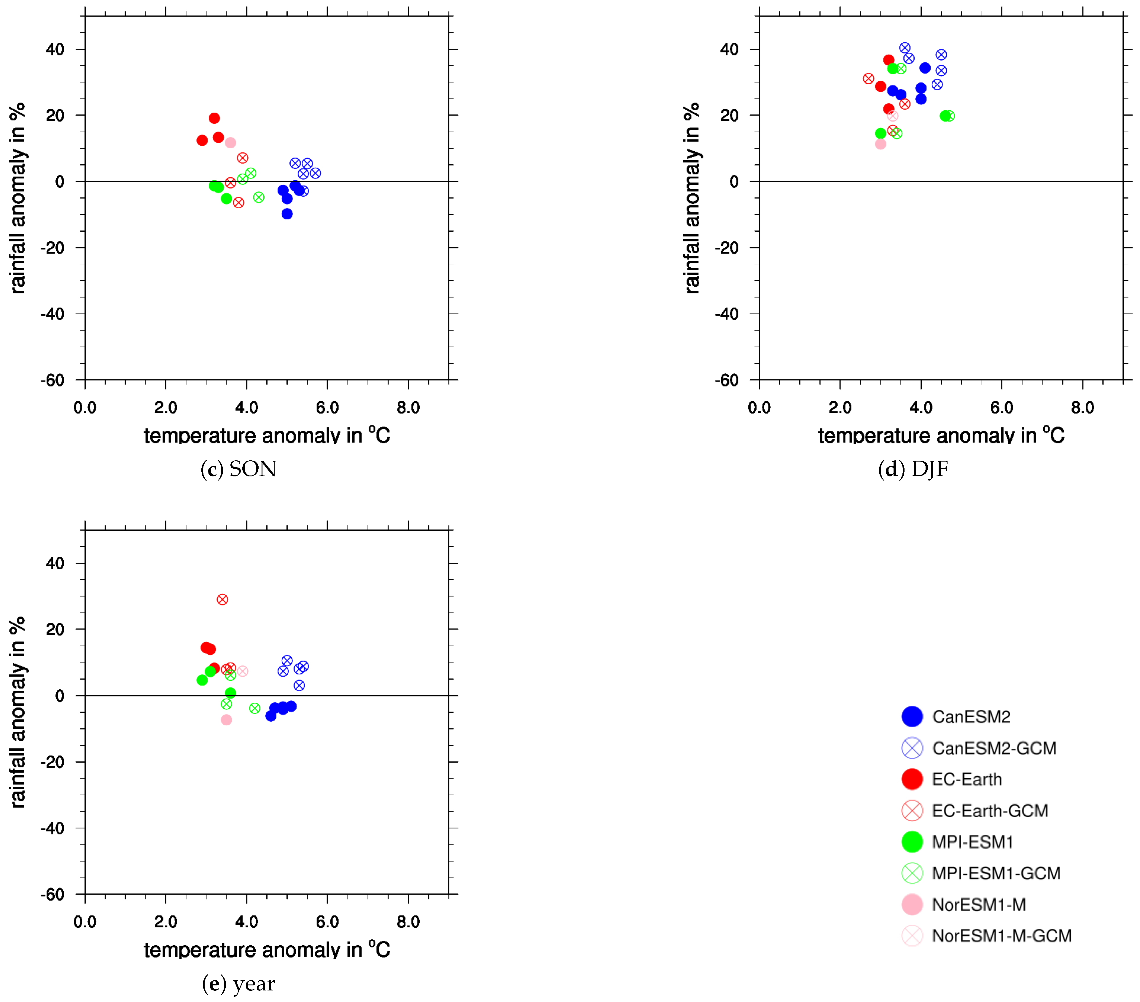
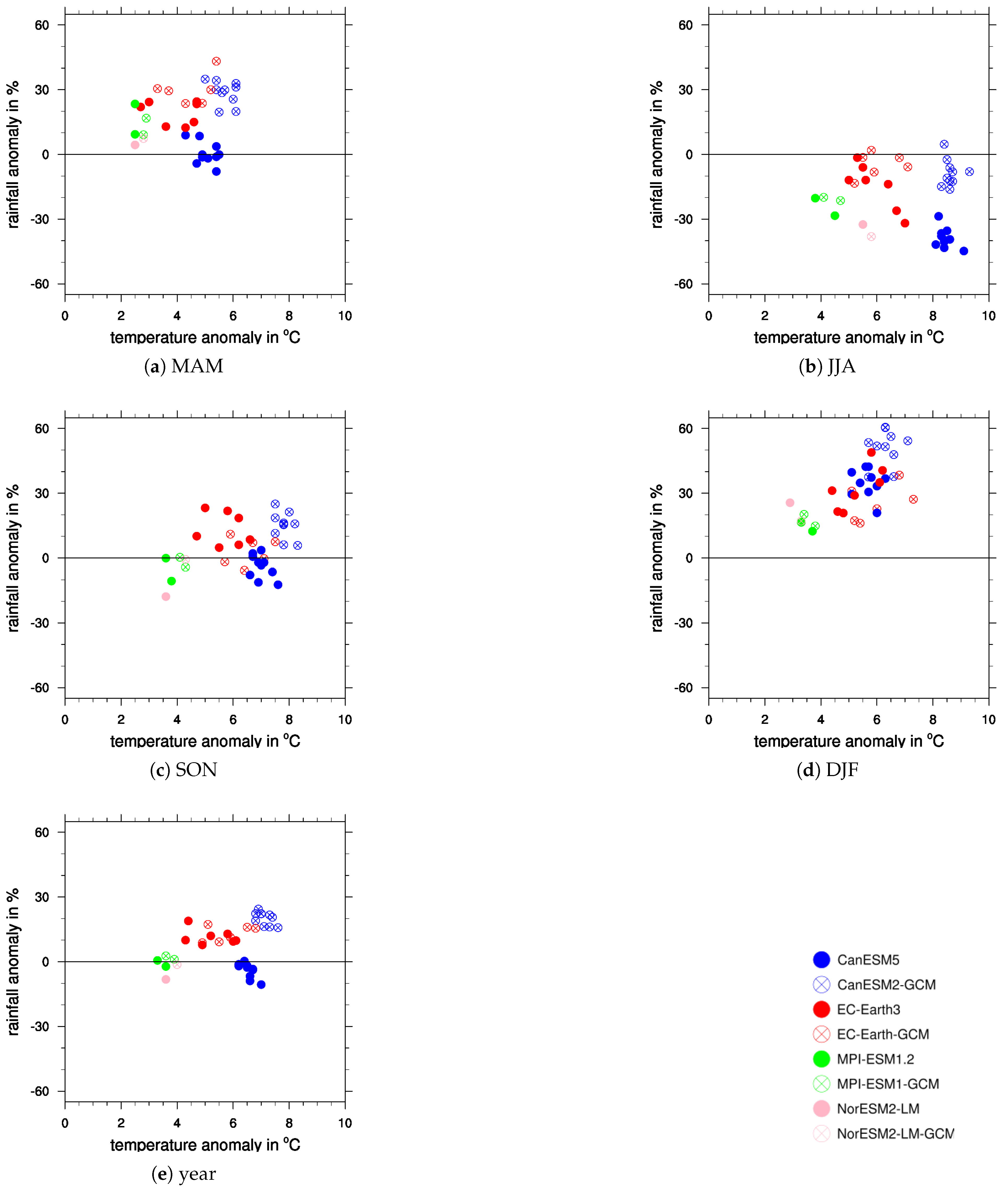
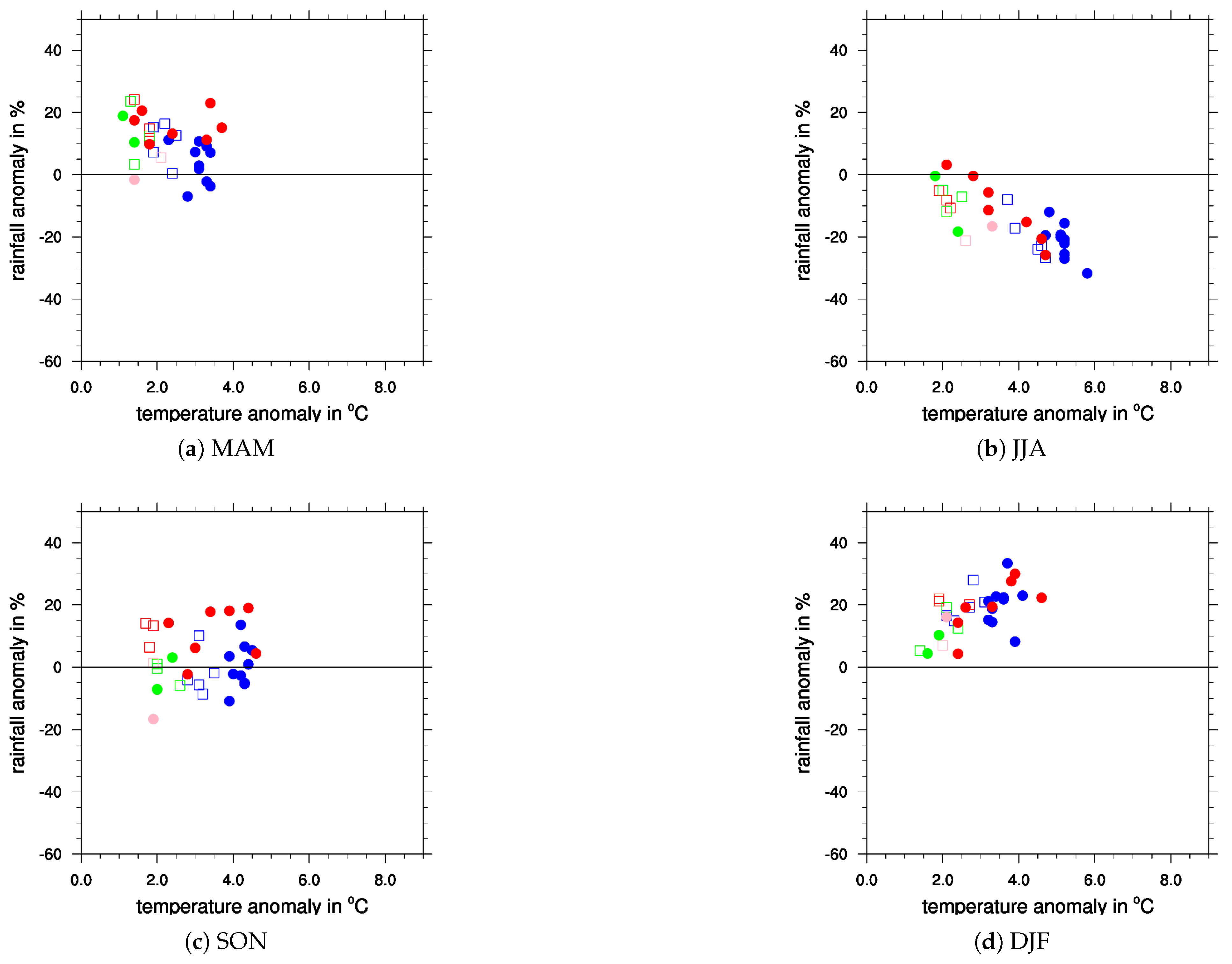
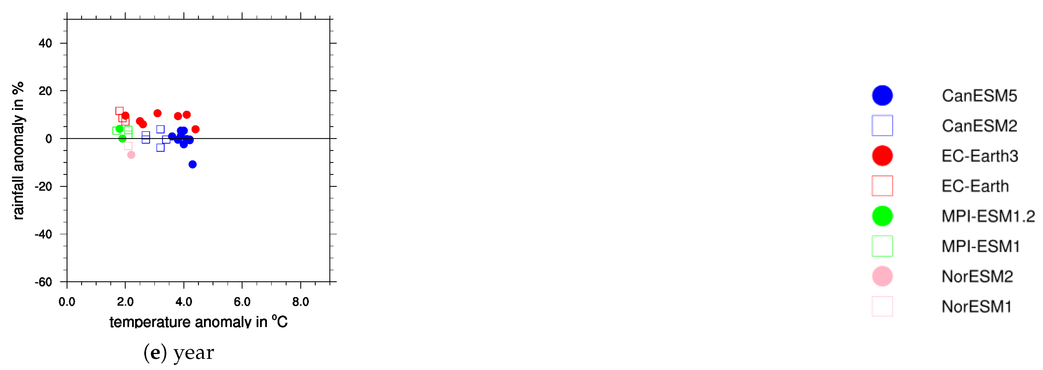
4.1. Comparing Global and Regional Change Signals

Differences between direct model results of the GCM and those downscaled with EPISODES are analysed in the following. For the analysis of GCM results, the Climate Data Operator (cdo) [37] was used in order to calculate a mean over a given area. (cdo fldmean -sellonlatbox,6,15,47.5,55 == area average over 6-15E/47.5-55N). The EPISODES downscaling method is applied, as detailed above. Please note that, unlike the GCM data, EPISODES produces missing values in the grid boxes outside of Germany that are ignored when calculating the area averages.
Figure 4 and Figure 5 show the change signal between 1971–2000 and 2071–2100 as a thermo-pluviogram for both scenarios (RCP8.5—CMIP5 and SSP5-8.5—CMIP6), respectively. It becomes apparent that the difference between the direct GCM output and EPISODES downscaled data is significantly larger in the case of SSP5-8.5 than under RCP8.5.
For temperature, there is a reduction of the change signal under EPISODES, which causes the downscaled values to be nearly up to 1 °C colder for both CMIP generations compared to the direct model output of the GCMs (RCP8.5 (Figure 4 and Table 3) and SSP5-8.5 (Figure 5 and Table 3)). This finding agrees with the results of [12,13].
The EPISODES downscaled precipitation fields are somewhat drier than the GCM results, in particular for the CMIP5 generation. This result agrees with the findings [16] for other ESD methods. In particular, the downscaled results of the CanESM runs have a climate change trend to drier conditions.

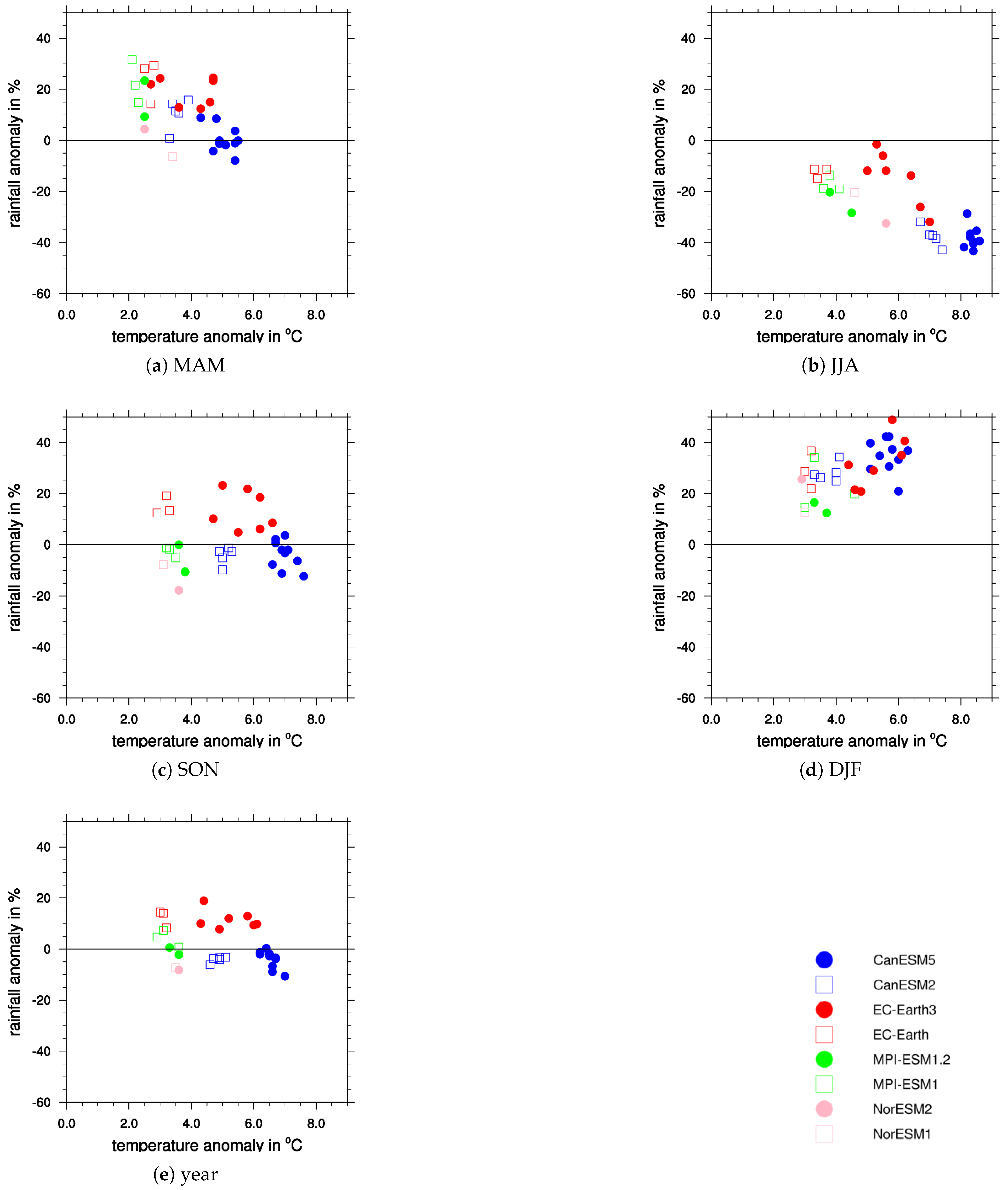
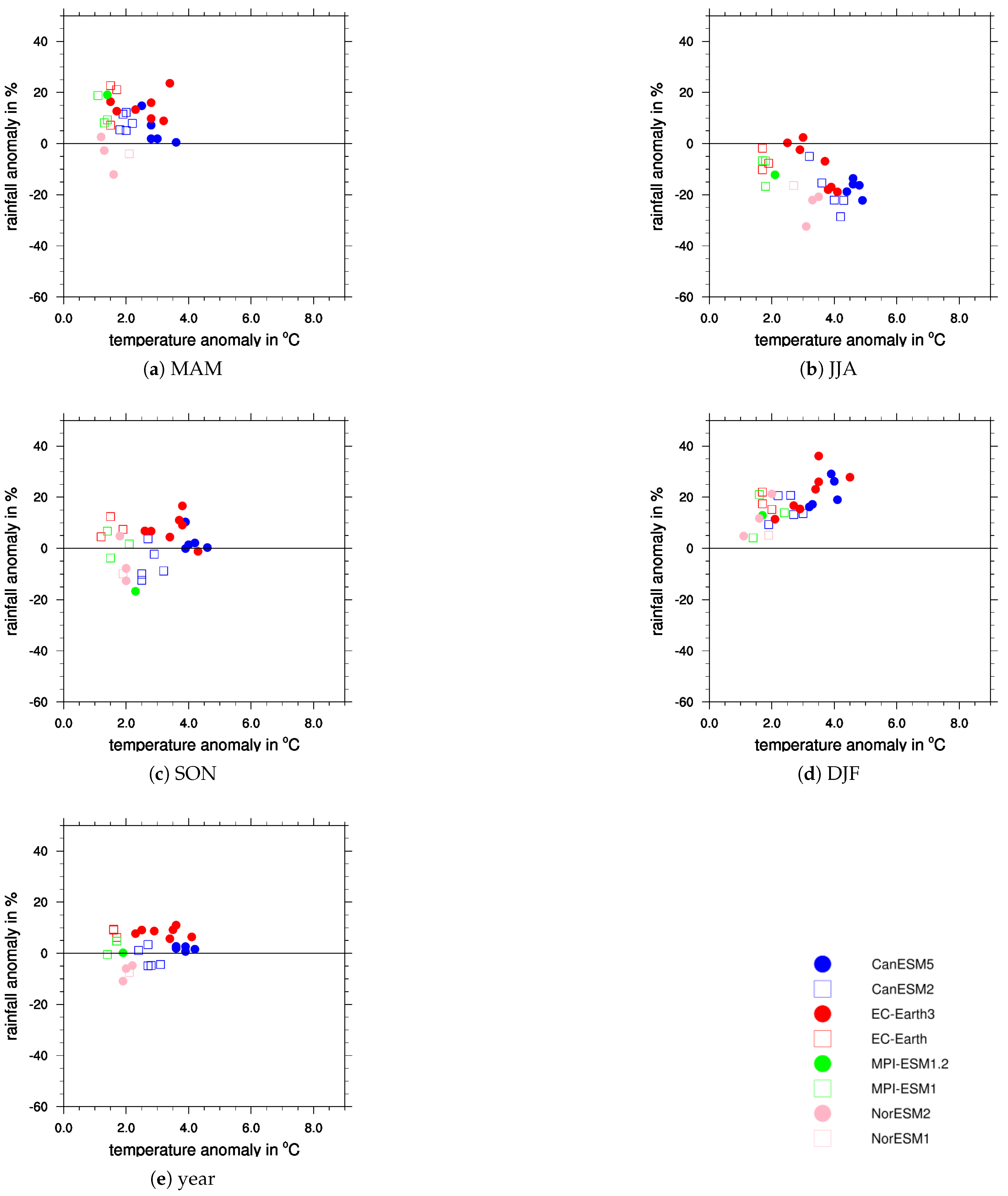
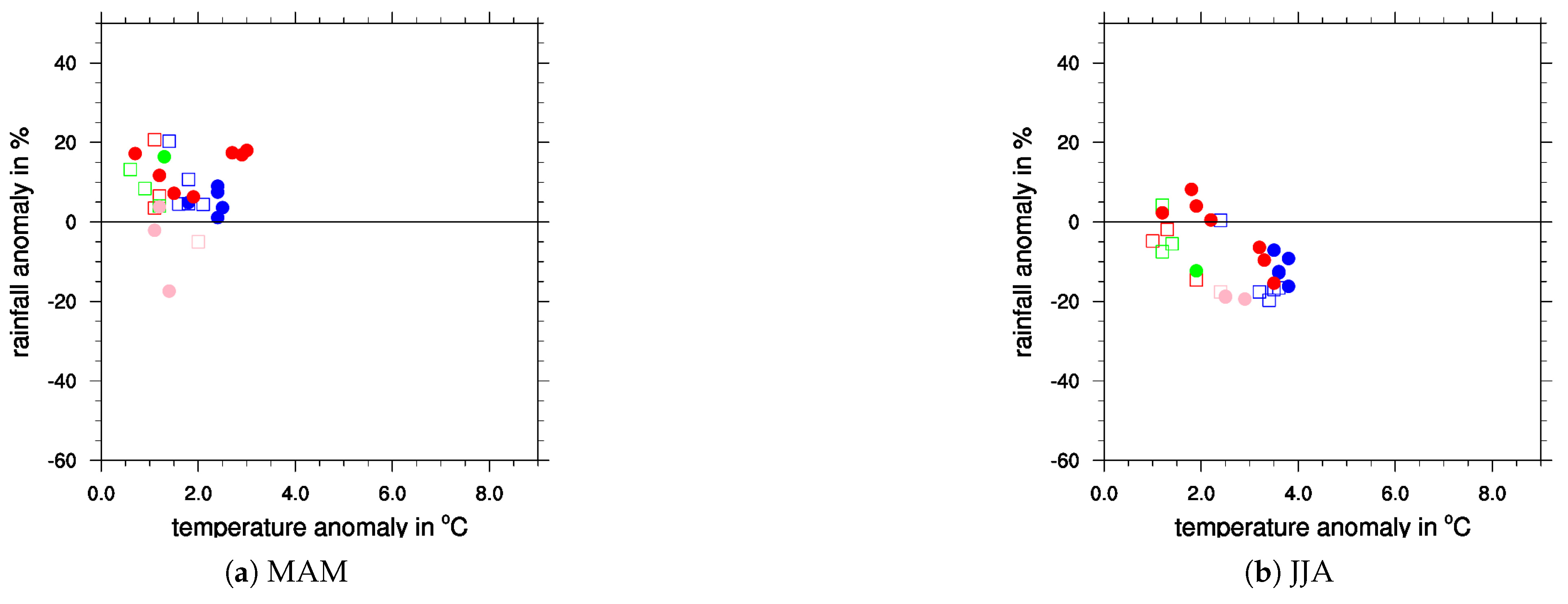
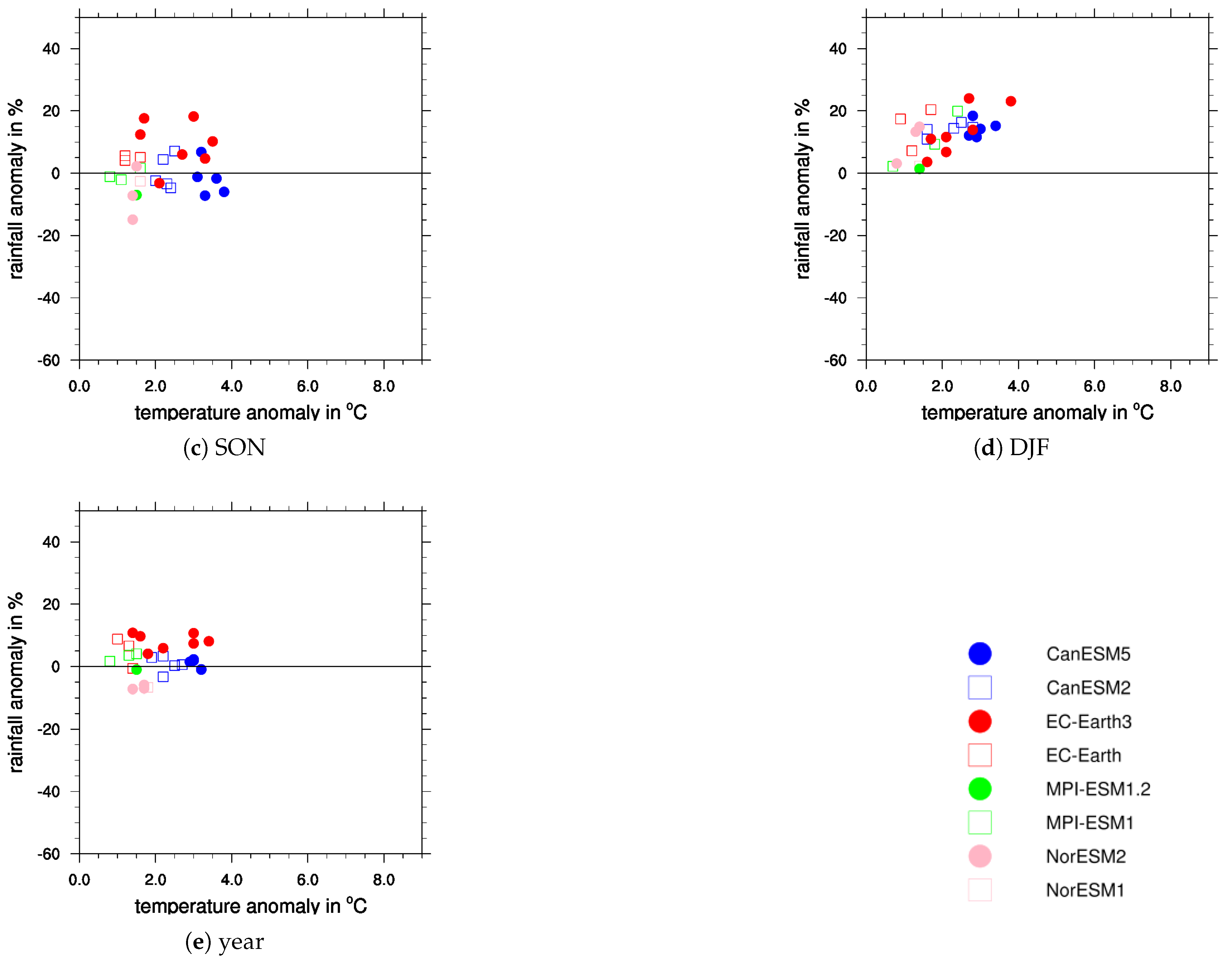
4.2. Comparing Regional CMIP5 and CMIP6 Signals

The change signals between CMIP5 and CMIP6 downscaled with EPISODES differ markedly in some cases, depending on GCM and season. In addition, the variability across different downscaled model runs for a given GCM is much larger for CMIP6 output, in particular for the CanESM and the EC-EARTH model.
The MPI-ESM and NorESM model display the smallest difference between the two CMIP generations. While there are hardly any differences with respect to temperature, the CMIP6 MPI-ESM model for the SSP5-8.5 scenario shows a tendency of less change in precipitation by the end of this century in comparison to CMIP5. For the same scenario, the CMIP6 NorESM model projects an increased seasonal variability in precipitation when compared to CMIP5, see Table 4.
The EC-EARTH model, which, under CMIP5, showed changes for Germany that are comparable to the results from the MPI-ESM model (compare Figure 6 and Figure 7), displays clear differences under CMIP6. The annual mean temperature signal increases by up to 3 °C at the end-century from RCP8.5 to SSP5-8.5. Under CMIP5, the yearly mean of the projected temperature increases by approximately +3 °C in the EC-EARTH model, whereas, under CMIP6, the projected changes are 4 to 6 °C—depending on the model realization. Seasonal changes for summer and autumn are even larger. The difference in the temperature change signal for EC-EARTH based on the scenario pair RCP4.5/SSP2-4.5 is generally lower when compared to RCP8.5/SSP5-8.5. With respect to precipitation, the change signal is very similar for the two CMIP generations and it varies for different scenarios.
Large differences between the two CMIP generations are also visible for CanESM. Changes in annual mean temperature for the scenario pair RCP8.5/SSP5-8.5 at the end of the century are approximately 1.7 °C higher under CMIP6. The signal varies across seasons: spring and summer are about 1.4 °C warmer, autumn and winter are almost 2 °C warmer (see Table 4). In absolute terms and with respect to 1971–2000, the new CanESM simulations project summer temperatures to increase by more than 9°C until the end of this century (see Figure 6b). The annual change in precipitation for CanESM remains almost unchanged. On the seasonal scale, CMIP6 projections show a slight increase of precipitation in winter that is balanced by a decrease in the summer. For the scenario pair RCP4.5/SSP2-4.5 and the mid-century period, the signals are weaker, but point in the same direction (see Figure 7).

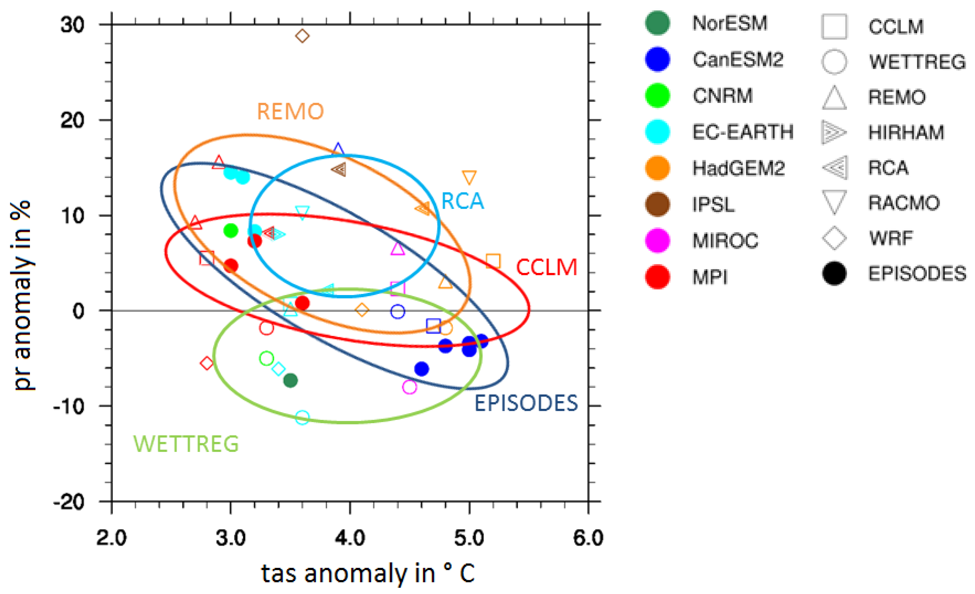
4.3. Internal Model-Chain Variability

The associated model-specific variability due to the spread projected by the different realizations also shows differences between CMIP5 and CMIP6. The analysis that is presented here is rather qualitative as the number of available realizations per GCM varies between the two CMIP generations (Table 2). Also note that only one CMIP5 realization for NorESM is available, such that NorESM is disregarded in this subsection. For the remaining GCMs, the difference in the internal model-chain variability between the two CMIP generations is the smallest for the MPI-ESM model (yearly values), both with respect to temperature and precipitation, compare Figure 6 and Figure 7. The remaining two GCMs (CanESM and EC-EARTH) show no to little increase in internal model variability for precipitation (yearly values), despite the fact that a larger number of realizations is available for CMIP6. However, with respect to temperature, EC-EARTH shows significant increases in internal model variability under CMIP6: The seven available SSP5-8.5 and SSP2-4.5 realizations both cover a range of about 2 °C (yearly values), as compared to less than 0.5 °C for the three available realizations under CMIP5. For CanESM there is no significant increase in temperature variability on the annual scale (given the larger number of CanESM realizations for CMIP6) and only slightly more variability on the seasonal scale.

5. Discussion

The four GCMs used in this study only represent a small part of the existing data. Therefore, it cannot be assumed that the results from these four GCMs provide a representative and comprehensive assessment of the climate change signal for Germany. However, they do provide a first indication of what is to be expected from the new generation of GCMs. Table 1 in [8] and Figure 4 in [9] show that our four models do not significantly differ from the other models in terms of ECS. According to both references, the four models used here cover a large part of the bandwidth of ECS variability.
Currently, an intensive discussion on the new CMIP6 model generation is underway. Several models have an ECS greater than five, as for the case of the CanESM5 model considered here, and some authors (e.g., [38]) argue for these values to be considered unrealistic. Others argue that while the probability of occurrence for such high ECS is low, it should still be considered within multi-model ensembles [39]. No assessment of the plausibility of the model runs used here is made within this article. From the authors’ point of view, we should wait for a final assessment by the IPCC within the framework of AR6.
The modified ECS is not the only reason for modified signals. According to Wyser et al. [17] ’ ... 50% or more of the temperature increase from CMIP5 to CMIP6 at the end of the century is due to changes in the prescribed GHG concentrations. The implication is that CMIP5 and CMIP6 projections for the 21st century are difficult to compare with each other not only as models differ, but also as the forcing conditions are not equal. Therefore, the communication of CMIP6 results to the impact, mitigation, and adaptation communities has to be carefully formulated, while taking into account the role of the updated GHG concentrations when interpreting the warmer climate projections for the 21st century.’
In this light, the data sets downscaled with EPISODES only represent a first step. In the course of the next years, a multitude of further downscaling activities are expected. Figure 1 shows that the different RCM and ESD techniques transform the underlying GCM signals slightly differently. Thus, we are curious to see how future studies compare to the results that are presented here.
However, in terms of climate change impacts, the new generation of climate models under CMIP6 as well as our analysis for Germany provide an alarming signal for society. An additional warming of about 2 °C (corresponding to the median warming observed here) would cause previously projected climate change impacts for the high-emission RCP8.5 scenario to occur already under the middle-of-the-road SSP2-4.5 scenario. According to the latest assessment (AR5) by the IPCC [40] and the current global warming target in 2100, in line with the Nationally Determined Contributions (NDCs), this would shift all of the impact categories considered by the IPCC’s burning ember diagram to high or very high risks.

6. Conclusions

The increases in ECS and corresponding stronger warming signal for some of the updated climate models contributing to CMIP6 are confirmed for the area of Germany. We observe clear increases in temperature signals for two out of four GCMs considered in our analysis. While almost no change in the temperature signal is found for the MPI-ESM and NorESM models across all scenarios considered, we find an additional temperature increase for the RCP 8.5/SSP5-8.5 scenario pair of about 1.7 °C and 3 °C for the CanESM and EC-EARTH model, respectively. Changes in the precipitation signals are less homogenous and show GCM-specific and season-specific trends. While we detect and quantify the effect of larger ECS for Germany, further research is required in order to identify the causal drivers behind this effect. In particular, the very large spread of internal variability between individual model implementations when compared to CMIP5 (about 2 °C for the EC-EARTH model analysed here) is striking and needs to be addressed. It is expected that the upcoming sixth assessment report (AR6) by the IPCC will provide more answers.

Author Contributions

F.K. and P.L. developed the downscaling method EPISODES. P.L. conducted the downscaling. F.K., P.L. and T.G. analysed the data and compiled the paper. All authors have read and agreed to the version of the manuscript.

Funding

This research received no external funding.

Acknowledgments

CMIP5 and CMIP6 data were obtained via the ESGF web site. The authors wish to thank all modelling groups for the provision of their results. We thank the EURO-CORDEX and ReKliEs-DE modelling groups for providing there results freely via the ESGF.

Conflicts of Interest

The authors declare no conflict of interest.

Appendix A. Additional Figures

Figure A1. Comparison of EPISODES downscaling results based on RCP8.5 (CMIP5) and SSP5-8.5 (CMIP6) for Germany. The symbols (open: CMIP5; filled: CMIP6) show the Germany-wide mean climate change signal in annual/seasonal precipitation and temperature for 2041–2070 with respect to 1971–2000. Different colours correspond to different GCMs. (Seasons: (a) spring (MAM), (b) summer (JJA), (c) autumn (SON), (d) winter (DFJ), (e) year).
Atmosphere 11 01245 g0a1aAtmosphere 11 01245 g0a1b
Figure A2. Comparison of EPISODES downscaling results based on RCP4.5 (CMIP5) and SSP2-4.5 (CMIP6) for Germany. The symbols (open: CMIP5; filled: CMIP6) show the Germany-wide mean climate change signal in annual/seasonal precipitation and temperature for 2041–2070 with respect to 1971–2000. Different colours correspond to different GCMs. (Seasons: (a) spring (MAM), (b) summer (JJA), (c) autumn (SON), (d) winter (DFJ), (e) year)).
Atmosphere 11 01245 g0a2aAtmosphere 11 01245 g0a2b

References

  1. Edwards, P. A Vast Machine—Computer Models, Climate Data, and the Politics of Global Warming; MIT Press: Cambridge, MA, USA, 2010. [Google Scholar]
  2. Von Storch, H. Climate models and modeling: An editorial essay. WIREs Clim. Chang. 2010, 1, 305–310. [Google Scholar] [CrossRef]
  3. Müller, P. Constructing climate knowledge with computer models. WIREs Clim. Chang. 2010, 1, 565–580. [Google Scholar] [CrossRef]
  4. Edwards, P. History of climate modeling. WIREs Clim. Chang. 2011, 2, 128–139. [Google Scholar] [CrossRef] [Green Version]
  5. Taylor, K.E.; Stouffer, R.J.; Meehl, G.A. An Overview of CMIP5 and the Experiment Design. Bull. Am. Meteor. Soc. 2012, 93, 485–498. [Google Scholar] [CrossRef] [Green Version]
  6. O’Neill, B.C.; Kriegler, E.; Riahi, K.; Ebi, K.L.; Hallegatte, S.; Carter, T.R.; Mathur, R.; van Vuuren, D.P. A new scenario framework for Climate Change Research: Scenario matrix architecture. Clim. Chang. 2014, 122, 387–400. [Google Scholar] [CrossRef] [Green Version]
  7. The CMIP6 landscape. Nat. Clim. Chang. 2019, 9, 727. [CrossRef] [Green Version]
  8. Flynn, C.M.; Mauritsen, T. On the Climate Sensitivity and Historical Warming Evolution in Recent Coupled Model Ensembles. Atmos. Chem. Phys. Discuss. 2020, 2020, 1–26. [Google Scholar] [CrossRef]
  9. CarbonBrief. CMIP6: The Next Generation of Climate Models Explained. 1999. Available online: https://www.carbonbrief.org/cmip6-the-next-generation-of-climate-models-explained (accessed on 16 November 2020).
  10. Zelinka, M.D.; Myers, T.A.; McCoy, D.T.; Po-Chedley, S.; Caldwell, P.M.; Ceppi, P.; Klein, S.A.; Taylor, K.E. Causes of Higher Climate Sensitivity in CMIP6 Models. Geophys. Res. Lett. 2020, 47, 1–12. [Google Scholar] [CrossRef] [Green Version]
  11. Meehl, G.A.; Senior, C.A.; Eyring, V.; Flato, G.; Lamarque, J.F.; Stouffer, R.J.; Taylor, K.E.; Schlund, M. Context for interpreting equilibrium climate sensitivity and transient climate response from the CMIP6 Earth system models. Sci. Adv. 2020, 6. Available online: https://advances.sciencemag.org/content/6/26/eaba1981.full.pdf (accessed on 16 November 2020). [CrossRef]
  12. Boé, J.; Somot, S.; Corre, L.; Nabat, P. Large discrepancies in summer climate change over Europe as projected by global and regional climate models: Causes and consequences. Clim. Dyn. 2020, 54, 2981–3002. [Google Scholar] [CrossRef]
  13. Sørland, S.L.; Schär, C.; Lüthi, D.; Kjellström, E. Bias patterns and climate change signals in GCM-RCM model chains. Environ. Res. Lett. 2018, 13, 074017. [Google Scholar] [CrossRef]
  14. Kreienkamp, F.; Paxian, A.; Früh, B.; Lorenz, P.; Matulla, C. Evaluation of the empirical–statistical downscaling method EPISODES. Clim. Dyn. 2019, 52, 991–1026. [Google Scholar] [CrossRef] [Green Version]
  15. Jacob, D.; Petersen, J.; Eggert, B.; Alias, A.; Christensen, O.B.; Bouwer, L.; Braun, A.; Colette, A.; Déqué, M.; Georgievski, G.; et al. EURO-CORDEX: New high-resolution climate change projections for European impact research. Reg. Environ. Chang. 2013, 1–16. [Google Scholar] [CrossRef]
  16. Hübener, H.; Bülow, K.; Fooken, C.; Früh, B.; Hoffmann, P.; Höpp, S.; Keuler, K.; Menz, C.; Mohr, V.; Radtke, K.; et al. ReKliEs-De Endbericht; Technical Report. Hessisches Landesamt für Naturschutz, Umwelt und Geologie: Wiesbaden, Germany, 2018. Available online: https://cera-www.dkrz.de/WDCC/ui/cerasearch/entry?acronym=ReKliEs-De_Ergebnisbericht (accessed on 16 November 2020).
  17. Wyser, K.; Kjellström, E.; Koenigk, T.; Martins, H.; Döscher, R. Warmer climate projections in EC-Earth3-Veg: The role of changes in the greenhouse gas concentrations from CMIP5 to CMIP6. Environ. Res. Lett. 2020, 15, 054020. [Google Scholar] [CrossRef]
  18. Mauritsen, T.; Roeckner, E. Tuning the MPI-ESM1.2 Global Climate Model to Improve the Match With Instrumental Record Warming by Lowering Its Climate Sensitivity. J. Adv. Model. Earth Syst. 2020, 12, e2019MS002037. Available online: https://agupubs.onlinelibrary.wiley.com/doi/pdf/10.1029/2019MS002037 (accessed on 16 November 2020). [CrossRef]
  19. Rauthe, M.; Steiner, H.; Riediger, U.; Mazurkiewicz, A.; Gratzki, A. A Central European precipitation climatology? Part I: Generation and validation of a high-resolution gridded daily data set (HYRAS). Meteorol. Z. 2013, 22, 235–256. [Google Scholar] [CrossRef]
  20. Frick, C.; Steiner, H.; Mazurkiewicz, A.; Riediger, U.; Rauthe, M.; Reich, T.; Gratzki, A. Central European high-resolution gridded daily data sets (HYRAS): Mean temperature and relative humidity. Meteorol. Z. 2014, 23, 15–32. [Google Scholar] [CrossRef]
  21. Eyring, V.; Bony, S.; Meehl, G.A.; Senior, C.A.; Stevens, B.; Stouffer, R.J.; Taylor, K.E. Overview of the Coupled Model Intercomparison Project Phase 6 (CMIP6) experimental design and organization. Geosci. Model Dev. 2016, 9, 1937–1958. [Google Scholar] [CrossRef] [Green Version]
  22. Cinquini, L.; Crichton, D.; Mattmann, C.; Harney, J.; Shipman, G.; Wang, F.; Ananthakrishnan, R.; Miller, N.; Denvil, S.; Morgan, M.; et al. The Earth System Grid Federation: An open infrastructure for access to distributed geospatial data. Future Gener. Comput. Syst. 2014, 36, 400–417. [Google Scholar] [CrossRef]
  23. Swart, N.C.; Cole, J.N.; Kharin, V.V.; Lazare, M.; Scinocca, J.F.; Gillett, N.P.; Anstey, J.; Arora, V.; Christian, J.R.; Jiao, Y.; et al. CCCma CanESM5 model output prepared for CMIP6 CMIP historical. Earth Syst. Grid Fed. 2019. [Google Scholar] [CrossRef]
  24. Swart, N.C.; Cole, J.N.; Kharin, V.V.; Lazare, M.; Scinocca, J.F.; Gillett, N.P.; Anstey, J.; Arora, V.; Christian, J.R.; Jiao, Y.; et al. CCCma CanESM5 Model Output Prepared for CMIP6 ScenarioMIP ssp245. 2019. Available online: https://cera-www.dkrz.de/WDCC/ui/cerasearch/cmip6?input=CMIP6.ScenarioMIP.CCCma.CanESM5.ssp245 (accessed on 16 November 2020).
  25. Swart, N.C.; Cole, J.N.; Kharin, V.V.; Lazare, M.; Scinocca, J.F.; Gillett, N.P.; Anstey, J.; Arora, V.; Christian, J.R.; Jiao, Y.; et al. CCCma CanESM5 Model Output Prepared for CMIP6 ScenarioMIP ssp585. 2019. Available online: https://cera-www.dkrz.de/WDCC/ui/cerasearch/cmip6?input=CMIP6.ScenarioMIP.CCCma.CanESM5.ssp585 (accessed on 16 November 2020).
  26. Hazeleger, W.; Guemas, V.; Wouters, B.; Corti, S.; Andreu-Burillo, I.; Doblas-Reyes, F.J.; Wyser, K.; Caian, M. Multiyear climate predictions using two initialization strategies. Geophys. Res. Lett. 2013, 40, 1794. [Google Scholar] [CrossRef]
  27. Doescher, R. The EC-Earth3 earth system model for the climate model intercomparison project 6. Manuscr. Prep. 2020; Unpublished work. [Google Scholar]
  28. EC-Earth Consortium (EC-Earth). EC-Earth-Consortium EC-Earth3 Model Output Prepared for CMIP6 CMIP Historical. 2019. Available online: https://cera-www.dkrz.de/WDCC/ui/cerasearch/cmip6?input=CMIP6.CMIP.EC-Earth-Consortium.EC-Earth3.historical (accessed on 16 November 2020).
  29. EC-Earth Consortium (EC-Earth). EC-Earth-Consortium EC-Earth3 Model Output Prepared for CMIP6 ScenarioMIP ssp245. 2019. Available online: https://cera-www.dkrz.de/WDCC/ui/cerasearch/cmip6?input=CMIP6.ScenarioMIP.EC-Earth-Consortium.EC-Earth3.ssp245 (accessed on 16 November 2020).
  30. EC-Earth Consortium (EC-Earth). EC-Earth-Consortium EC-Earth3 Model Output Prepared for CMIP6 ScenarioMIP ssp585. 2019. Available online: https://cera-www.dkrz.de/WDCC/ui/cerasearch/cmip6?input=CMIP6.ScenarioMIP.EC-Earth-Consortium.EC-Earth3.ssp585 (accessed on 16 November 2020).
  31. Wieners, K.H.; Giorgetta, M.; Jungclaus, J.; Reick, C.; Esch, M.; Bittner, M.; Legutke, S.; Schupfner, M.; Wachsmann, F.; Gayler, V.; et al. MPI-M MPI-ESM1.2-LR Model Output Prepared for CMIP6 CMIP Historical. 2019. Available online: https://cera-www.dkrz.de/WDCC/ui/cerasearch/cmip6?input=CMIP6.CMIP.MPI-M.MPI-ESM1-2-LR.historical (accessed on 16 November 2020).
  32. Wieners, K.H.; Giorgetta, M.; Jungclaus, J.; Reick, C.; Esch, M.; Bittner, M.; Gayler, V.; Haak, H.; de Vrese, P.; Raddatz, T.; et al. MPI-M MPI-ESM1.2-LR Model Output Prepared for CMIP6 ScenarioMIP ssp245. 2019. Available online: https://cera-www.dkrz.de/WDCC/ui/cerasearch/cmip6?input=CMIP6.ScenarioMIP.MPI-M.MPI-ESM1-2-LR.ssp245 (accessed on 16 November 2020).
  33. Wieners, K.H.; Giorgetta, M.; Jungclaus, J.; Reick, C.; Esch, M.; Bittner, M.; Gayler, V.; Haak, H.; de Vrese, P.; Raddatz, T.; et al. MPI-M MPI-ESM1.2-LR Model Output Prepared for CMIP6 ScenarioMIP ssp585. 2019. Available online: https://cera-www.dkrz.de/WDCC/ui/cerasearch/cmip6?input=CMIP6.ScenarioMIP.MPI-M.MPI-ESM1-2-LR.ssp585 (accessed on 16 November 2020).
  34. Seland, Ø.; Bentsen, M.; Oliviè, D.J.L.; Toniazzo, T.; Gjermundsen, A.; Graff, L.S.; Debernard, J.B.; Gupta, A.K.; He, Y.; Kirkevåg, A.; et al. NCC NorESM2-LM Model Output Prepared for CMIP6 CMIP Historical. 2019. Available online: https://cera-www.dkrz.de/WDCC/ui/cerasearch/cmip6?input=CMIP6.CMIP.NCC.NorESM2-LM.historical (accessed on 16 November 2020).
  35. Seland, Ø.; Bentsen, M.; Oliviè, D.J.L.; Toniazzo, T.; Gjermundsen, A.; Graff, L.S.; Debernard, J.B.; Gupta, A.K.; He, Y.; Kirkevåg, A.; et al. NCC NorESM2-LM Model Output Prepared for CMIP6 ScenarioMIP ssp245. 2019. Available online: https://cera-www.dkrz.de/WDCC/ui/cerasearch/cmip6?input=CMIP6.ScenarioMIP.NCC.NorESM2-LM.ssp245 (accessed on 16 November 2020).
  36. Bentsen, M.; Oliviè, D.J.L.; Seland, Ø.; Toniazzo, T.; Gjermundsen, A.; Graff, L.S.; Debernard, J.B.; Gupta, A.K.; He, Y.; Kirkevåg, A.; et al. NCC NorESM2-MM Model Output Prepared for CMIP6 ScenarioMIP ssp585. 2019. Available online: https://cera-www.dkrz.de/WDCC/ui/cerasearch/cmip6?input=CMIP6.ScenarioMIP.NCC.NorESM2-MM.ssp585 (accessed on 16 November 2020).
  37. Uwe, S. Climate Data Operators (CDO) User Guide; Technical Report; DKRZ: Hamburg, Germany, 2019; p. 222. Available online: https://code.mpimet.mpg.de/projects/cdo/embedded/cdo.pdf (accessed on 17 November 2020).
  38. Zhu, J.; Poulsen, C.J.; Otto-Bliesner, B.L. High climate sensitivity in CMIP6 model not supported by paleoclimate. Nat. Clim. Chang. 2020, 10, 378–379. [Google Scholar] [CrossRef]
  39. Forster, P.M.; Maycock, A.C.; McKenna, C.M.; Smith, C.J. Latest climate models confirm need for urgent mitigation. Nat. Clim. Chang. 2020, 10, 7–10. [Google Scholar] [CrossRef]
  40. IPCC. Climate Change 2013: The Physical Science Basis. Contribution of Working Group I to the Fifth Assessment Report of the Intergovernmental Panel on Climate Change; Technical Report; Intergovernmental Panel On Climate Change: Cambridge, UK, 2013; p. 1535. Available online: http://www.climatechange2013.org/images/report/WG1AR5_ALL_FINAL.pdf (accessed on 10 February 2014).
Figure 1. Comparison of the results of different downscaling methods based on CMIP5 for Germany depicted as a Thermo-Pluviogram. The symbols compare the Germany-wide mean climate change signal in annual precipitation (pr) and temperature (tas) under RCP8.5 for 2071–2100 with respect to 1971–2000. Different colours correspond to different Global Climate Models (GCMs), while different marker styles label different downscaling methods. The ellipses are added for guidance to highlight the method-specific relation between temperature increase and precipitation change. Based on data from the EURO-CORDEX [15] and ReKliEs-De project [16].
Atmosphere 11 01245 g001
Figure 2. Downscaled results for the modeling chain historical—CanESM5 run1—EPISODES2018. Shown are the yearly mean values over the period 1971–2000 for (a) precipitation (pr) and (b) temperature (tas).
Atmosphere 11 01245 g002
Figure 3. Downscaled results for the modeling chain SSP5-8.5—CanESM5 run1—EPISODES2018. Shown is the change between 2071–2100 and 1971–2000 (future minus past) for northern hemisphere summer (JJA) for (a) precipitation (pr) and (b) temperature (tas).
Atmosphere 11 01245 g003
Figure 4. Comparison of the direct GCM output (crossed circles) and EPISODES downscaling results (filled circles) based on RCP8.5 (CMIP5) for Germany. The symbols show the Germany-wide mean climate change signal in annual/seasonal precipitation and temperature for 2071–2100 with respect to 1971–2000. Different colours correspond to different GCMs. (Seasons: (a) spring (MAM), (b) summer (JJA), (c) autumn (SON), (d) winter (DFJ), and (e) year).
Atmosphere 11 01245 g004aAtmosphere 11 01245 g004b
Figure 5. Comparison of the direct GCM output (crossed circles) and EPISODES downscaling results (filled circles) based on SSP5-8.5 (CMIP6) for Germany. The symbols show the Germany-wide mean climate change signal in annual/seasonal precipitation and temperature for 2071–2100 with respect to 1971–2000. Different colours correspond to different GCMs. (Seasons: (a) spring (MAM), (b) summer (JJA), (c) autumn (SON), (d) winter (DFJ), and (e) year).
Atmosphere 11 01245 g005
Figure 6. Comparison of EPISODES downscaling results based on RCP8.5 (CMIP5) and SSP5-8.5 (CMIP6) for Germany. The symbols (open: CMIP5; filled: CMIP6) show the Germany-wide mean climate change signal in annual/seasonal precipitation and temperature for 2071–2100 with respect to 1971–2000. Different colours correspond to different GCMs. (Seasons: (a) spring (MAM), (b) summer (JJA), (c) autumn (SON), (d) winter (DFJ), and (e) year).
Atmosphere 11 01245 g006
Figure 7. Comparison of EPISODES downscaling results based on RCP4.5 (CMIP5) and SSP2-4.5 (CMIP6) for Germany. The symbols (open: CMIP5; filled: CMIP6) show the Germany-wide mean climate change signal in annual/seasonal precipitation and temperature for 2071–2100 with respect to 1971–2000. Different colours correspond to different GCMs. (Seasons: (a) spring (MAM), (b) summer (JJA), (c) autumn (SON), (d) winter (DFJ), and (e) year).
Atmosphere 11 01245 g007
Table 1. Possible reasons for the differences in ECS between the CMIP5 and CMIP6 models studied here according to [11].
ModelReasons for Change in ECS since CMIP5
MPI-ESM1.2Tuned with cloud parameters to be the same as CMIP5. Pretuned version had ECS = 7 caused by a positive low-cloud feedback in the tropics.
EC-Earth3Early indications of the role of cloud-aerosol interactions.
CanESM5Large increase since CMIP5 model (3.7–5.6)—at least half seems to be related to cloud feedback increase.
NorESM2-LMSmall decrease since CMIP5 model (2.9–2.5), which is not yet understood.
Table 2. Overview of the GCMs analysed for the two scenario pairs RCP4.5 + SSP2-4.5 and RCP8.5 + SSP5-8.5, respectively. Note that the second model run for MPI-ESM1-2-HR under SSP2-4.5 is currently unavailable.
CMIP5CMIP6
CanESMCanESM2 (r1 to r5)CanESM5 [23,24,25] (r1 to r10)
EC-EARTHEC-EARTH [26] (r2, r9, r12)EC-EARTH3-veg [27,28,29,30] (r1, r4, r6, r9, r11, r13, r15)
MPI-ESMMPI-ESM-LR (r1 to r3)MPI-ESM1-2-HR [31,32,33] (r1 and r2)
NorESMNCC-NorESM1-M (r1)NorESM2-LM [34,35,36] (r1 to r3)
Table 3. Mean (annual and seasonal) difference of the EPISODES downscaling results and the direct GCM output (EPISODES trend minus GCM trend) for temperature (tas) and precipitation (pr), as observed in Figure 4 and Figure 5. Seasons are defined as follows: spring (MAM), summer (JJA), autumn (SON), winter (DJF).
CMIP6 SSP5-8.5tas (Change in °C)pr (Change in %)
2071–2100MAMJJASONDJFyearMAMJJASONDJFyear
CanESM−0.6−0.2−0.8−0.6−0.6−28−30−19−18−24
EC-EARTH−0.5−0.1−0.8−0.7−0.5−11−101010−2
MPI-ESM−0.4−0.3−0.5−0.1−0.33−4−3−3−3
NorESM−0.3−0.3−0.7−0.4−0.4−36−179−7
CMIP5 RCP8.5tas (Change in °C)pr (Change in %)
2071–2100MAMJJASONDJFyearMAMJJASONDJFyear
CanESM−0.4−0.1−0.4−0.4−0.3−11−13−7−8−12
EC-EARTH−0.5−0.2−0.6−0.1−0.40−4156−3
MPI-ESM−0.4−0.6−0.8−0.2−0.6129−204
NorESM0.40.10.50.30.4101920915
Table 4. Multi-realization-mean annual and seasonal difference in the GCM-specific climate change signal for temperature (tas) and precipitation (pr) between CMIP5 and CMIP6 (mean CMIP6 climate signal minus mean CMIP5 climate signal). Seasons are defined, as follows: spring (MAM), summer (JJA), autumn (SON), and winter (DJF).
SSP5-8.5/RCP8.5tas (Change in °C)pr (Change in %)
2041–2070MAMJJASONDJFyearMAMJJASONDJFyear
CanESM0.90.91.10.91.0−7−220−1
EC-EARTH0.81.51.71.11.3−1−30−2−1
MPI-ESM−0.3−0.10.0−0.2−0.12−10−5−1
NorESM−0.70.70.00.10.1−75−189−4
SSP5-8.5/RCP8.5tas (Change in °C)pr (Change in %)
2071–2100MAMJJASONDJFyearMAMJJASONDJFyear
CanESM1.51.41.91.91.7−10−1070
EC-EARTH1.32.52.62.22.1−5−2−23−1
MPI-ESM0.30.30.4−0.10.3−6−7−3−8−5
NorESM−0.91.00.5−0.10.111−12−1013−1
SSP2-4.5/RCP4.5tas (Change in °C)pr (Change in %)
2041–2070MAMJJASONDJFyearMAMJJASONDJFyear
CanESM0.60.41.10.80.8−43−200
EC-EARTH0.91.01.21.11.1354−23
MPI-ESM0.40.60.3−0.20.38−9−6−9−4
NorESM−0.80.2−0.2−0.2−0.20−1−480
SSP2-4.5/RCP4.5tas (Change in °C)pr (Change in %)
2071–2100MAMJJASONDJFyearMAMJJASONDJFyear
CanESM1.00.81.41.21.1−31904
EC-EARTH1.01.62.01.41.6−3−20−20
MPI-ESM0.10.30.6-0.10.37−2−18−9−3
NorESM−0.70.60.0−0.3−0.10−9580
Publisher’s Note: MDPI stays neutral with regard to jurisdictional claims in published maps and institutional affiliations.

