Analysis of Spatial Data from Moss Biomonitoring in Czech–Polish Border

Abstract

The purpose of the study was the analysis of spatial data gained by biomonitoring with the use of mosses. A partial goal was set to characterize the regional atmospheric deposition of pollutants in the air based on the results of the analyses and simultaneously verify the suitability of using mosses as an alternative for monitoring air quality in smaller industrial areas. In total, 93 samples of moss were collected and examined from the area of the Moravian–Silesian Region in the Czech Republic and the area of the Silesian Voivodship in Poland. The samples were analyzed using instrumental neutron activation analysis. Based on the analyses performed, 38 elements, which had been evaluated using principal component analysis, hierarchical clustering on principal components, factor analysis, correlation analysis, contamination factor, geoaccumulation index, enrichment factor, and pollution load index, were determined. The analyses resulted in a division of elements into a group with its concentrations close to the level of the values of the natural background and the second group of elements identified as emission likely originating from anthropogenic activity (Sm, W, U, Tb, and Th). The likely dominant source of emissions for the studied area was identified. Simultaneously, the results pointed to sources of local importance. The area of interest was divided into clusters according to the prevailing type of pollution and long-distance transmission of pollutants was confirmed.

1. Introduction

The environment as a complex and interconnected system consists of natural, artificial, and social components. Over the years, there has been observed an overall imbalance in the environment. In practice, monitoring especially of anthropogenic pollutants is a complex process. First, the sources and emissions are identified; then the risks are assessed. Critical emissions are controlled and economic aspects are integrated at the same time. Technical field measurements require equipment and are associated with high costs. Among the wide range approaches that make it possible to assess the state of the atmosphere, biological monitoring, i.e., biomonitoring, is increasingly coming to the fore. The complexity and at the same time the relative simplicity of its application make it an ideal tool for the given purpose. Compared to technical monitoring methods, it is inexpensive. Among the organisms used to monitor the state of the atmosphere, bryophytes are one of the most widely used. Mosses do not have a cuticle and root system and thus obtain nutrients in particles or solution directly from atmospheric deposition. They have good bioaccumulation ability, the concentration in the insole reflects the deposition from the atmosphere without being affected by soil concentrations [1].

Currently, the most problematic air pollutants in the urban environment are fine dust particles (Particulate matter). Particulate matter is the result of complex reactions of chemicals such as sulfur dioxide and nitrogen oxides, which are pollutants emitted from power plants, industries, and automobiles. They are compounds from trace elements such as Cd, Co, Cr, Cu, Fe, Mn, Pb, Sb and Zn [2] or Al, Sb, As, Cd, Fe, Mn, Ni, Pb, Cu, V, Zn according to [3]. According to the European Environment Agency (EEA) map representing the average annual concentrations of PM₁₀ in 2016 (Figure 1), the areas with the highest airborne dust loads are Poland, within the Czech Republic, the Moravian–Silesian Region. Further north Italy, Bulgaria, Macedonia, Greece and Turkey.

Air quality in the Moravian–Silesian Region, especially in the Ostrava and Karviná regions, has been unsatisfactory for a long time. This fact is also evidenced by the map of average annual concentrations of PM₁₀ for the Czech Republic in 2018 (Figure 2). This is mainly due to the high concentration of industry in a densely populated area, but transport and heating of households also have an impact.

The territory of the city of Ostrava belongs into the area of the Ostrava Basin, which is a slightly warm area with southwest and northeast wind directions. The landscape is open to the north and northeast, which causes a negative effect of northern winds in winter, but also in summer. The territory of Ostrava belongs into a moderately warm climatic region, but differs with certain peculiarities caused by a high concentration of industry, dense construction and specific conditions of the Ostrava Basin.

According to the database of the Register of Emissions and Air Polution Sources (REZZO), it is evident that primary emissions of solid pollutants are from large industrial sources, as well as local heating plants with a share of about 30%. A large share is not attributed to emissions of solids from transport. Total emissions in the Ostrava–Karviná agglomeration are approximately five times higher than in the Prague agglomeration and eight times higher than in the Brno agglomeration [6]. The Moravian–Silesian Region is characterized by the highest concentrations of PM_2.5 and PM₁₀ and, compared to other regions, high values of benzo(a)pyrene appear. Directly in Ostrava, the limit value for benzene and arsenic is also repeatedly exceeded.

The aim of the paper is the analysis of spatial data obtained by biomonitoring using mosses. Furthermore, on the basis of the performed analyzes, characterization of the regional atmospheric deposition of pollutants in the air on the Czech–Polish border and verification of the suitability of the use of bryophytes as alternative monitors of air quality in small industrial areas. The another aims are identification of the significance of individual groups of sources of pollutant emissions and determination of the extent and location of polluted areas. The study evaluates the measured data and determines whether the elements contained in the samples are of natural origin, i.e., if they are part of the natural background, or whether they are of anthropogenic origin and determines whether the resulting values are of local origin or come from long-distance transmission.

The research was carried out in frame of the dissertation thesis [7].

2. Materials and Methods

2.1. Study Area

In 2015, a sampling area was selected and a network of sampling points was created on the Czech–Polish border (Figure 3), areas with the highest airborne dust loads in Europe, using GIS technologies. More species of moss were also collected from one locality for the possibility of comparing sorption capacity of different species. The assessment of the difference between the individual species is not the subject of this article. The network was also extended to locations where pollution was not expected.

2.2. Sampling and Sample Preparation

A total of 44 samples were taken from 41 sampling sites in a regular network on an area of 1600 km² (40 × 40 km). In 2016, the network was expanded by another 44 sampling points, where a total of 50 moss samples were taken (Figure 4). All sampling was performed according to the Monitoring Manual issued by the International Cooperative Programme (ICP) Vegetation program [8]. Sampling was performed in a square network with a side size of 60 km, with an area of 3600 km², where the points are a maximum of 10 km apart. A total of 85 localities were sampled, 94 moss samples were taken. According to the sampling manual, it is recommended for national monitoring to collect 1.5 samples of moss per 1000 km², if this is not possible, two samples in the area of 50 km × 50 km could be collected. For this research, it was sampled in a non-standard dense network, to characterize the regional atmospheric deposition of pollutants in the air. In the first campaign in 2015, the species Hypnum cupressiforme, Brachythecium rutabulum, Hylocomium splendens, Cirriphyllum piliferum, Calliergonella cuspidata, Rhytidiadelphus squarrosus, Atrichum undulatum, Eurhinchium hians were collected. In 2016, only Pleurozium schreberi, Hypnum cupressiforme, and Brachythecium rutabulum were collected. The necessity to use species different from recommended in the manual, is due to the dense sampling network, which extends to areas unfavorable for the growth of the recommended species, for example in city centers.

Each sampling site was selected at least 3 m from the involved treetop, preferably on the ground or surface of decaying trunks. Coarse dirt was removed in the field. According to the methodology, sampling points should be located outside urban areas, at least 300 m from main roads, villages, and industry and at least 100 m from smaller roads and houses, but these conditions could not always be met. One composite sample was prepared from each site from five to ten samples collected on an area of 50 m × 50 m. Only one species of moss was present in the composite sample. The collection was carried out in paper or plastic breathable bags. The amount of moss from one locality was one liter. Powder-free gloves were used during collection.

Samples cleaned of coarse impurities were dried in the laboratory at room temperature (20–25 °C). When handling the samples, it was necessary to avoid the use of metal aids to not contaminate the samples. The moss was cleaned of all remnants of forest bedding. Only the green parts, which represent the most frequent increments over the last three years, were taken from the sample for analysis. A sample of 6 g was weighed from the thus treated material, which was then sealed in polyethylene bags and taken to the Joint Institute for Nuclear Research (JINR) in Dubna, Russian Federation.

2.3. Neutron Activation Analysis

At the JINR, the sample was processed in a chemical laboratory, where 2 × 0.3 g of each sample was weighed. With the help of a compression piston, these two samples were compressed into sampling tablets. One was then wrapped in a polyethylene bag to determine elements with short lived isotopes (SLI) and the other in an aluminum film to determine long lived isotope (LLI). Irradiation of the sample for SLI analysis lasted 3 min and the subsequent measurement of emitted $\gamma$-radiation took place for 15 min. Irradiation of samples intended for LLI analysis lasted 3–4 days and subsequent measurement of emitted $\gamma$-radiation was performed twice, after 3 days and after 21 days for 30 and 90 min, respectively. Semiconductor high pure germanium (HPGe) detectors from CANBERRA were used for the measurement. The GENIE 2000 program was used to process γ spectra. The quality control of Neutron activation analysis (NAA) results was ensured by simultaneous analysis of the examined samples and standard reference materials (SRM) of National Institute of Standards and Technology (NIST) and Institute for Reference Materials and Measurements (IRMM): NIST SRM 1515-Apple Leaves, NIST SRM 1547-Peach Leaves, NIST SRM 1575a-Pine Needles, NIST SRM 1633b-Coal Fly Ash, NIST SRM 1633c-Coal Fly Ash, NIST SRM 1632c-Coal (Bituminous), NIST SRM 2709-San Joaquin Soil, NIST SRM 2710-Montana Soil, NIST SRM 2711-Montana Soil, SRM 2891-Copper Sand, IRMM BCR 667-Estuarine Sediment.

2.4. Statistical Data Processing

Results of NAA are in mass concentrations. Concentrations are in the form of composition data, which are defined as vectors with positive components. Components quantitatively describe parts of an entity carrying only relative information [9]. Most statistical methods are constructed assuming Euclidean geometry [10]. The special character of compositional data, different sample space, and geometry requires a different approach than standard multidimensional data, where the data are absolute. The first comprehensive approach was introduced by John Aitchison, namely log-ratio analysis [11]. Unlike other transformation methods, the identification of individual variables is impossible because it is reduced by one variable. However, to express the overall similarity between the elements measured at each site, isometric transformation is most appropriate. The basic idea is to express the composition using a suitably chosen class of transformations as real vectors and subsequent data processing is possible by common statistical methods [12].

Environmental pollution indices [13], namely Contamination factor (CF), Geoaccumulation index (Igeo), Enrichment factor (EF), and Pollution load index (PLI), make it possible to distinguish elements whose concentrations correspond to the natural background and elements whose concentrations indicate pollution on a spatial scale. The combination of these factors was used, for example, for the assessment of heavy metals levels in the sediment of the Jazmurian playa region in southeastern Iran by Shirani et al. [13] or Jiang et al. [14] in the characterization of pollution and identification of heavy metals in soil. Individual factors were used in studies of atmospheric deposition using bryophytes, e.g., [15,16,17,18,19].

Statistical data processing was performed in the R studio version 3.6.1 and the statistical software STATISTICA 10. R is a freely available programming language and software environment for statistical calculations and graphics. R was created by Ross Ihaka and Robert Gentleman at the University of Auckland, New Zealand, and is developed by the R Development Core Team [20]. R contains many functions for data manipulation, calculations, and graphical outputs. Many other features are included in support packages.

To allow relative multidimensional data analysis, which requires data with Euclidean geometry, the data were transformed according to the principle of compositional data analysis. Specifically, the Isometric log-ratio transformation was used for the transformation, which allows expressing the composition in an orthonormal coordinate system. The “robComposition” package was used for transformation [21]. Exploitation analysis of data, extraction, and visualization of Principal Component Analysis (PCA) and Hierarchical Clustering on Principal Components (HCPC) were performed using the “factoextra” and “FactoMineR” packages [22]. The “corrplot” package was used to create a correlation matrix with a correlogram [23]. Factor analysis was performed in the STATISTICA program. It is a comprehensive system containing tools for data management, analysis, visualization, and development of user applications, originally developed by StatSoft, which was gain by Dell in March 2014 [24]. Before the calculation of the factor analysis itself, the data were rotated. Varimax type rotation was performed. It is an orthogonal rotation that minimizes the number of variables that have high loads with each factor in common. It is calculated by the sum of the variances of the factor load squares in the individual columns.

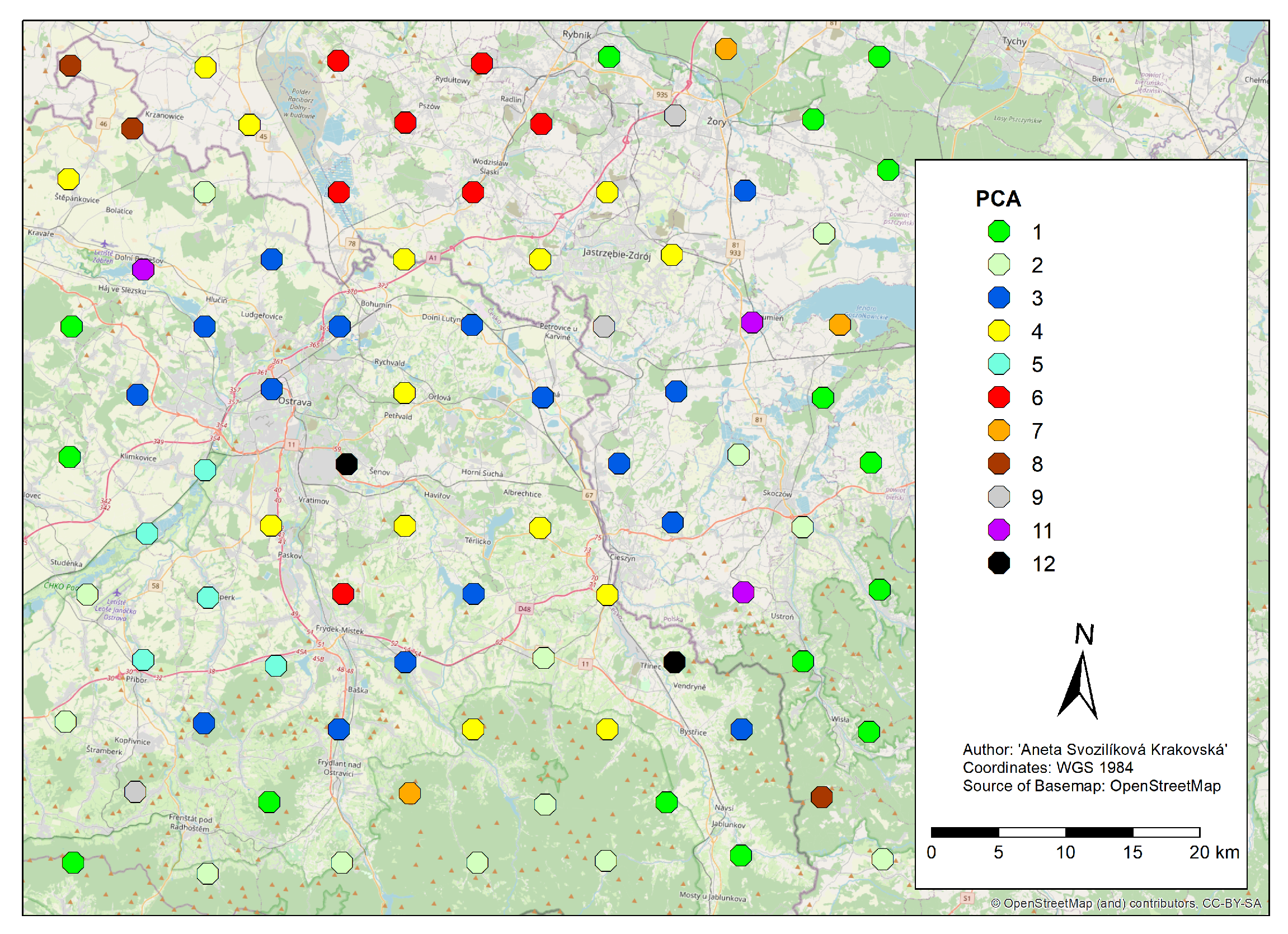
2.4.1. Principal Component Analysis

The main goal is to simplify the description of a group of mutually linear dependent, i.e., correlated features. The motivation is to replace a large number of input variables with a much smaller number of new variables, so-called components, without much loss of essential information about the input data. It is a method of a linear transformation of the original characters into new, uncorrelated variables, called main components. Each main component represents a linear combination of the original features, the basic characteristic of each of them is its degree of variability, i.e., variance. The principal component method is one of the basic multi-elemental analysis used in the evaluation of atmospheric deposition using biomonitoring [25,26].

2.4.2. Factor Analysis

Factor analysis (FA) is a widely used method in evaluating the resulting concentrations from biomonitoring using bryophytes, e.g., [27,28,29,30]. Factor analysis is a multidimensional statistical method, explaining the variance of observed variables using a smaller number of potential variables—the factors. Its essence is the analysis of the structure of mutual variables based on the assumption that these dependencies are the result of a certain smaller number of background immeasurable factors. These factors are called common factors. The goal is to reduce the number of variables and reveal the structure of the relationship between variables. Factor analysis can to some extent be considered an extension of the principal component method (PCA), but unlike PCA, it is based on an attempt to explain the relationship between variables. The shortcomings of PCA include that it is dependent on changes in the scale of variables. The factor analysis approach makes it possible to eliminate this shortcoming. The weaknesses of factor analysis lie in the ambiguity of the estimation of factor parameters (i.e., the dependence of the FA result on the rotation used) and in the need to specify the number of common factors before performing the analysis. The advantages of FA are greater economy and generality. Like PCA, the problem is the interpretation of the factor if the variables do not have a multidimensional normal distribution. The main goal of PCA is to explain the maximum variability of data, the main goal of FA is to explain the covariance between variables. The basis of factor analysis is the assumption that the observed covariances between variables are the result of the action of common factors and not the relationship between variables. Thus, the FA assumes that variables are a linear combination of hypothetical variables-factors [31,32,33].

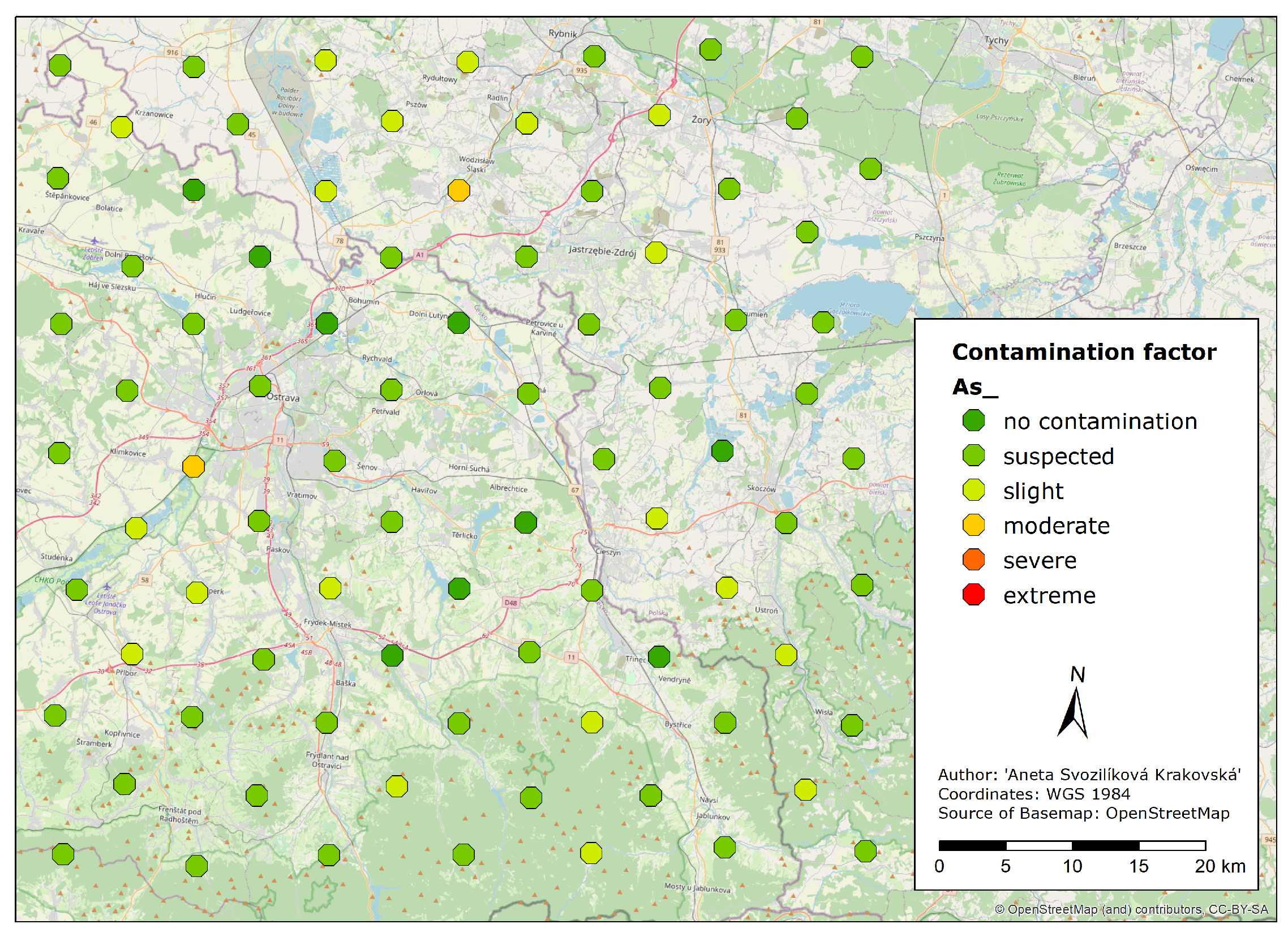
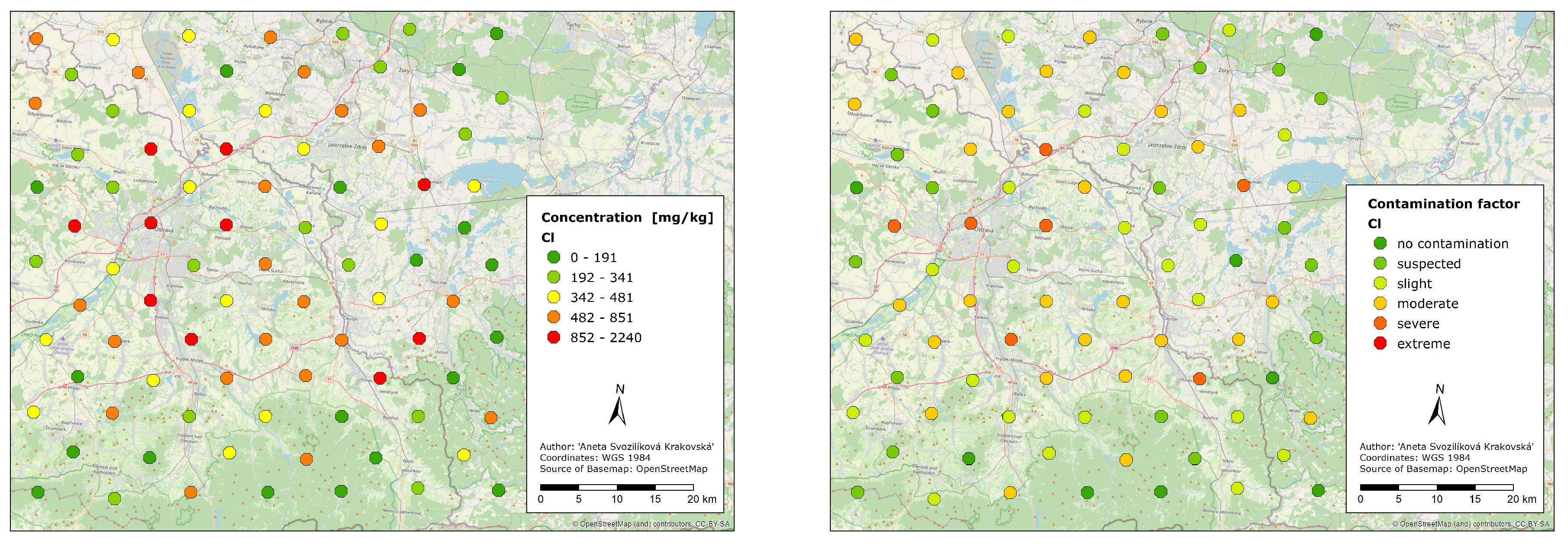
2.4.3. Contamination Factor

Contamination factor was first used by Hakanson [34] to study the pollution of reservoirs and to determine which ones need more attention in terms of potential environmental risk. To evaluate the degree of contamination of bryophytes used for air biomonitoring, the use of CF for the first time described by Fernandez et al. [35]. According to these authors, a scale was used to categorize individual sampling points. The contamination factor evaluates the degree of contamination for individual elements, but also the degree of contamination for individual sampling points. This allows you to compare data from different regions. It is calculated as the ratio of the concentration of the element in the moss and the background value of the element in the studied area.

$$\mathrm{CF}=\frac{\mathrm{concentration}}{\mathrm{background}}$$

(1)

2.4.4. Geoaccumulation Index

The Geoaccumulation Index (I_geo) was originally introduced by Müller [36] to determine and define metal contamination in sediments by comparing current concentrations with pre-industrial values. It is calculated according to the formula [37]:

$$\mathrm{Igeo}=lo{g}_2\left[\frac{c_{\mathrm{n}}}{1.5B_{\mathrm{n}}}\right]$$

(2)

• c_n concentration in moss sample n,
• B_n background value for moss sample n,
• a factor of 1.5 is used due to possible variability in background values.

2.4.5. Enrichment Factor

Given that some authors, e.g., Covelli and Fontolan [38] criticize the use of Igeo to assess the degree of contamination and suggest the use of normalized values, the present article also used a method of comparing the ratio of individual metals to a reference element that is probably of geogenic origin, and the impact of metals on the environment. The degree of pollution was determined using the Enrichment factor (EF). EF is a standardized method proposed by Sinex and Helz [39] to assess metal concentrations. The concentration of metals is usually normalized as a ratio to another component of the sediment. Rubio et al. [40] stated that there is no general agreement on the most suitable sediment component to be used for normalization. The most usable are Al, Fe, total organic carbon, and sediment grain size. However, an important criterion is the non-anthropogenic origin of the element. The component chosen for this purpose should not be variable depending on anthropogenic activity [41]. For this reason, the use of the given elements as comparative elements was excluded, as their occurrence in the examined area may be influenced by the presence of the metallurgical industry. Therefore, the scandium element was selected for comparison, which has a relatively small application in industry, and although it reached high values in the calculation of the contamination and geoaccumulation factor, this was probably due to swirling dust and contamination of samples with soil particles. The crustal origin of scandium is confirmed by the results of a biomonitoring study such as Olise et al. [42]. Several studies have been performed using scandium as a reference element [43,44]. The formula for calculating EF is:

$$\mathrm{EF}=\frac{{\left(\frac{\mathrm{metal}}{\mathrm{Sc}}\right)}_{\mathrm{sample}}}{{\left(\frac{\mathrm{metal}}{\mathrm{Sc}}\right)}_{\mathrm{background}}}$$

(3)

where $\left(\frac{\mathrm{metal}}{\mathrm{Sc}}\right)$_sample is the ratio of metal to concentration of Sc in the sample and $\left(\frac{\mathrm{metal}}{\mathrm{Sc}}\right)$_background is the ratio of metal to concentration of Sc in the reference samples.

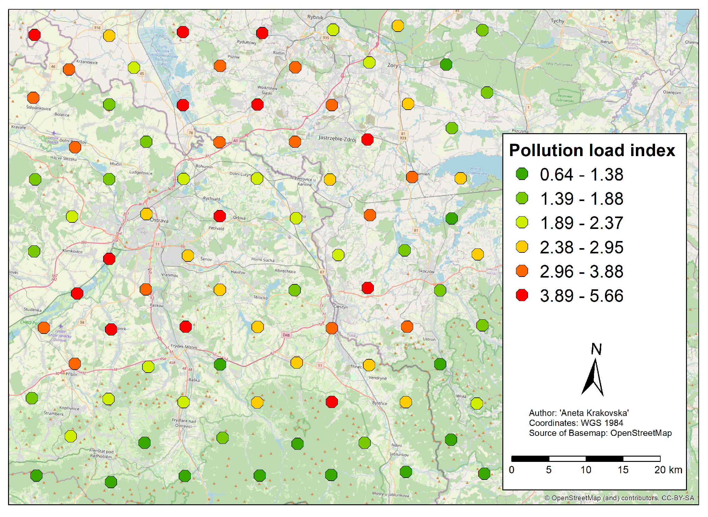
2.4.6. Pollution Load Index

The Pollution Load Index (PLI) was designed and tested to assess the heavy metal pollution of estuaries. Tomlinson [45] stated that although there are many indicators to facilitate the detection of heavy metal pollution, there are significant problems in evaluating the heavy metal load on rivers. The interpretation of the results is complicated by differences in the composition of species and conditions in different places, differences in the period of sampling, or the age of organisms and methods of storing metals in the bodies of organisms. For the biomonitoring of air pollutants using mosses and lichens, PLI was used, for example, by Salo [46], who studied the relationship between the concentration of anthropogenic magnetic particles and heavy metals and compared the correlations between magnetic sensitivity and PLI. The Tomlinson contamination index [47] indicates the extent to which a sample exceeds the concentrations of heavy metals in the natural environment and indicates the overall state of toxicity for the sample [46]. PLI is defined as the square root of the product of the contamination factors for a given sample:

$$\mathrm{PLI}=\sqrt[n]{CF1\times CF2\times CF3\times \dots CFn}$$

(4)

where CF indicates contamination factors for a single site sample.

3. Results

In 2015, a total of 44 samples were taken from 41 sites. In 2016, another 50 samples were taken from 44 localities. Concentrations of 38 elements were obtained for samples from 2015, and 47 elements were evaluated in 2016. Due to incomplete data, given the uncertainties in the neutron activation analysis, the elements, Yb, Lu, Hg, Cu, Zr, In, Eu, Gd, and Dy, were removed from further processing. The sampling point CZT-15-13-01 was also removed, as it was collected and analyzed separately and the resulting concentrations and composition of the elements are different from other sampling points. 93 samples were entered into statistical analyzes and 38 variables (elements) were evaluated. The basic numerical characteristics of the analyzed data are given in the (

Table 1. Descriptive statistics of measurement, n = 93.

	Min [mg/kg]	Max [mg/kg]	Mean [mg/kg]	Median [mg/kg]	std.dev [mg/kg]	var [mg/kg]2	var. koef. /	Skew /	kurt. /
										Na	84.9	1150	276	224	173	29,869	0.6	2	9.1
Mg	789	4790	2525	2340	1009	1,017,205	0.4	0.3	2.1
Al	305	11,000	2530	1830	2119	4,488,235	0.8	1.4	4.9
Cl	69.3	2240	502	389	394	154,875	0.8	1.9	7.7
K	4660	20,200	11,024	11,100	3104	9,634,437	0.3	0.1	3
Ca	1540	10,600	5941	5940	2411	5,811,460	0.4	0	2
Sc	0.053	1.86	0.51	0.41	0.384	0.147	0.8	1.1	3.8
Ti	22.3	923	202	133	177	31,182	0.9	1.5	5.2
V	0.551	14.9	4	2.88	3.13	9.78	0.8	1.2	4.1
Cr	1.1	34.1	6.84	5.41	5.56	30.96	0.8	2.1	8.9
Mn	45.7	767	230	195	153	23,449	0.7	1.5	5
Fe	338	18,700	2203	1680	2258	5,099,947	1	4.5	31.9
Co	0.119	2.13	0.76	0.63	0.483	0.233	0.6	1.1	3.6
Ni	0.711	8.26	2.98	2.69	1.465	2.15	0.5	1.2	4.8
Zn	30.6	587	111	85.4	106	11,295	1	3.3	13.6
As	0.286	3.75	1.07	0.97	0.518	0.269	0.5	2.1	10
Se	0.06	2.39	0.64	0.39	0.537	0.289	0.8	1.4	3.8
Br	1.65	7.73	3.54	3.27	1.31	1.72	0.4	1	3.9
Rb	5.94	63.8	17.2	13.3	11.5	132	0.7	1.9	6.8
Sr	5.65	69.2	27.4	26.6	13.3	177	0.5	0.5	3
Mo	0.016	1	0.39	0.34	0.245	0.06	0.6	0.6	2.3
Cd	0.02	7.09	1.18	0.57	1.719	2.95	1.5	2.2	6.8
Sb	0.049	1.31	0.34	0.28	0.226	0.051	0.7	2	7.8
I	0.349	4.08	1.41	1.31	0.724	0.525	0.5	1	4.2
Cs	0.078	1.74	0.41	0.33	0.282	0.079	0.7	1.7	7.4
Ba	13.1	209	63.1	55.8	33.8	1145	0.5	1.3	5.8
La	0.194	6.13	1.6	1.24	1.211	1.47	0.8	1.2	4.1
Ce	0.011	15.6	3.23	2.43	2.682	7.19	0.8	1.6	6.6
Nd	0.249	6.82	1.91	1.74	1.333	1.78	0.7	1	4.1
Sm	0.026	1.03	0.26	0.2	0.201	0.04	0.8	1.3	4.5
Tb	0.003	0.16	0.04	0.03	0.03	0.001	0.8	1.3	4.5
Tm	0.002	0.08	0.02	0.02	0.017	0	0.7	1.2	4.2
Hf	0.025	1.56	0.39	0.27	0.34	0.115	0.9	1.2	3.9
Ta	0.004	0.21	0.05	0.04	0.041	0.002	0.8	1.3	4.4
W	0.03	1.38	0.27	0.23	0.233	0.054	0.9	2.2	9.9
Au	0	0.07	0	0	0.008	0	4.4	7.4	59.4
Th	0.049	1.92	0.49	0.38	0.4	0.16	0.8	1.3	4.5
U	0.021	0.56	0.18	0.14	0.14	0.02	0.8	1	3.3

).

The values of the coefficient of variation express the inhomogeneous character of the data set. The skewness coefficient for some elements (e.g., Cr, Fe, Zn, As, Cd, W, and Au) indicates a positive skewness of the data set, this fact is also evidenced by higher values of averages than the median values. Based on the results of the sharpness coefficient, it can be concluded that the distribution is more pointed than normal. These facts are also confirmed by frequency histograms. It is evident from the histograms that the data for most elements do not have a normal or Gaussian distribution according to the author Carl Friedrich Gauss.

To allow relative multivariate data analysis, which requires Euclidean geometry data, a nonlinear data transformation was performed according to the principle of compositional data analysis. Specifically, the Isometric log-ratio transformation was used for the transformation.

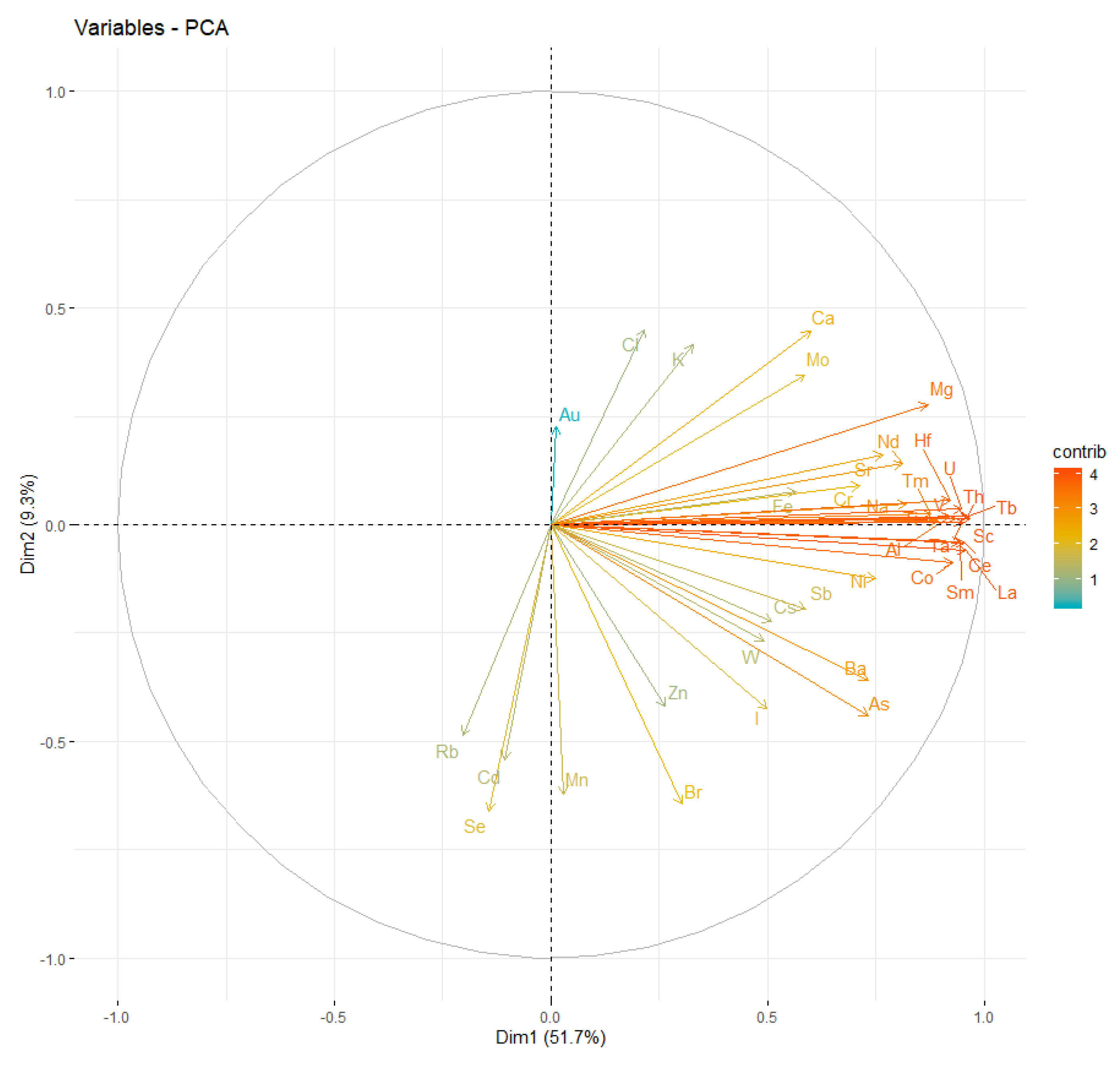
3.1. Principal Component Analysis

Scree graph analysis, i.e., a bar graph of eigenvalues, was used to identify the number of major components, where the break point from rapid descent to gradual determines the number of “useful” components. The useful components are thus separated by a distinct break point, and the x coordinate of this break is the index value sought. In this case, two. The biplot is a natural consequence of the singular value decomposition of a matrix [48]. The Scatterplot (Figure 5) shows the component weights for the two main components and allows to compare the distances between the variables. Short distance means a strong correlation. Sampling points located far from the origin of coordinates are extremes (CZT15-11-01, CZT15-03-01, PLS16-45-01, PLS16-83-01), the closest, on the other hand, are the most typical. The sites located in the diagram close to each other are similar, far from each other are different. Sites located clearly in one cluster are similar, yet dissimilar to objects in other clusters. Isolated sites (PLS16-83-01) may be strongly dissimilar to others unless there is an apparent inhomogeneity due to skewed data. The color scale distinguishes the quality of the data representation in the graph.

The Plot Components Weight (Figure 6) shows the component weights for the first two main components. The distances between the variables are compared, shorter means a strong correlation. Variables close to the origin are of little importance (Au). Variables with an angle of 0° between their guides are completely positively correlated. The group of elements U, Sc, Ta, Al, Co, Sm, Ce, La, V, Th, Tm, Tb have a strong correlation with each other. Also the elements Fe, Cr, Na, Sr, Nd, Ni, Sb and Cs are correlated with the mentioned group, but they are no longer of such significance. Variables with an angle of 90° are completely uncorrelated and variables with an angle of 180° are negatively correlated, for example Au, Cl, K to Rb, Cd, Se, Mn. The color scale indicates the level of contribution of the element to the main component.

A principal component analysis was performed for the three major components. Subsequently, hierarchical clustering was performed on these three components. The individual sites are visualized on the graph of the main components (Figure 7) and the individual clusters are color-coded. The map shows a better division of the sampling points into clusters (Figure 8).

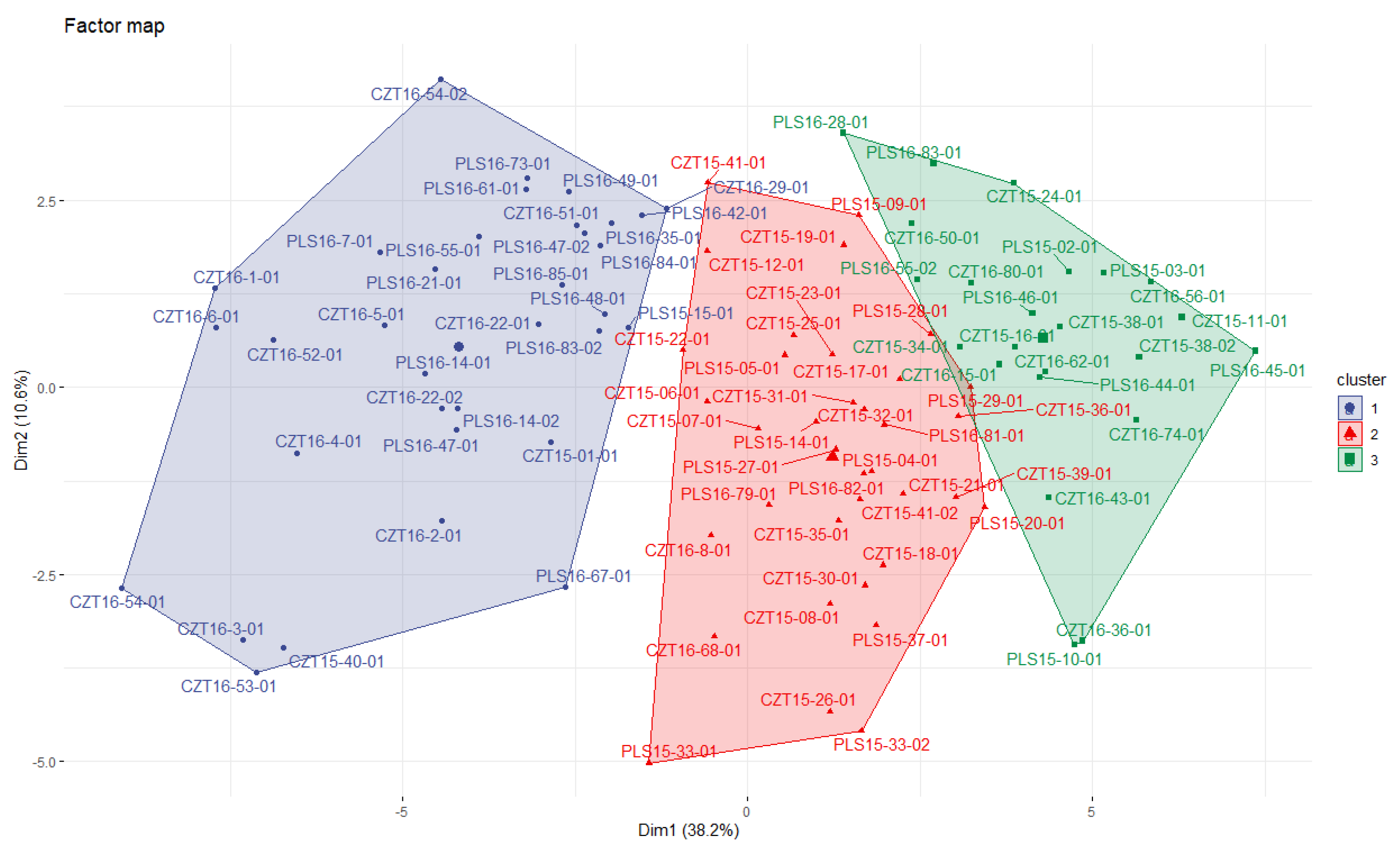
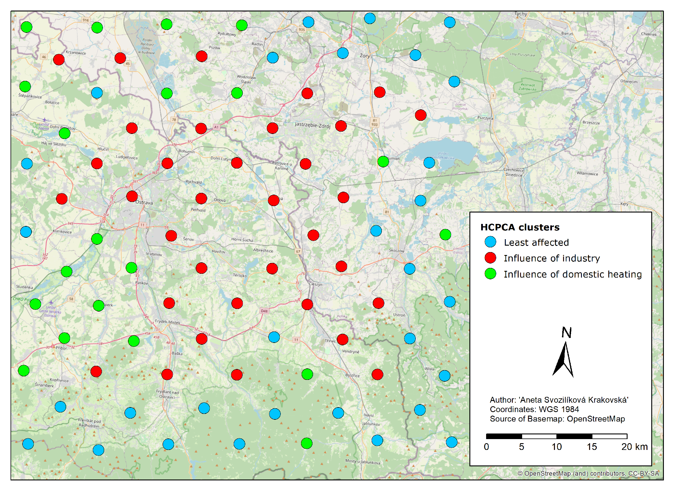
3.2. Factor Analysis

Factor analysis was performed in the software STATISTICA. The optimal number of factors to be retained was determined by plotting line rubble-Scree plot [49] eigenvalues of all factors. The ideal number of factors can be determined at the point in the graph where the highest decrease in eigenvalues is between the two factors. The biggest break is between one and two factors and another only between the fifth and sixth factors, so the factor analysis was performed for five factors.

Prior to the analysis itself, the data were rotated to clearly distinguish the load pattern, i.e., to differentiate the factors indicated by the high load for some variables and low load for others. Namely, Varimax normalized rotation was used. As a result, those variables (elements) whose load was greater than 0.6 for a given factor were selected (

Table 2. Factor loads of individual elements, n = 93.

	Factor 1	Factor 2	Factor 3	Factor 4	Factor 5
Na	0.79	0.16	0.16	0.07	0.13
Mg	0.76	0.07	0.37	0.05	0.39
Al	0.94	0.04	0.13	−0.06	0.07
Cl	0.11	−0.02	0.12	0.08	0.82
K	0.25	0.07	0.00	0.22	0.79
Ca	0.37	0.01	0.72	0.03	0.42
Sc	0.96	0.11	0.19	0.01	0.03
Ti	0.92	0.03	0.08	−0.09	0.11
V	0.91	0.08	0.25	−0.07	0.03
Cr	0.56	0.13	0.62	0.03	−0.13
Mn	−0.08	0.61	−0.12	−0.33	−0.03
Fe	0.38	0.19	0.65	0.09	−0.17
Co	0.85	0.26	0.30	−0.01	−0.04
Ni	0.67	0.39	0.18	0.19	−0.08
Zn	0.07	0.81	0.00	0.13	0.10
As	0.65	0.62	0.00	0.03	−0.13
Se	−0.08	0.09	−0.17	−0.74	−0.37
Br	0.20	0.63	−0.14	−0.45	0.11
Rb	−0.12	0.41	−0.55	0.17	−0.26
Sr	0.58	0.22	0.48	−0.03	0.35
Mo	0.36	0.17	0.70	0.29	0.13
Cd	−0.09	0.09	−0.16	−0.82	−0.01
Sb	0.36	0.55	0.48	0.10	−0.13
I	0.28	0.58	0.39	−0.33	−0.05
Cs	0.47	0.36	0.09	0.24	−0.33
Ba	0.61	0.59	0.05	−0.13	0.17
La	0.95	0.18	0.12	−0.06	0.10
Ce	0.96	0.13	0.11	−0.04	0.06
Nd	0.83	−0.08	0.19	−0.05	0.12
Sm	0.96	0.09	0.10	−0.10	0.07
Tb	0.97	0.10	0.15	0.00	0.07
Tm	0.89	0.14	0.05	0.12	0.08
Hf	0.91	0.12	0.13	0.03	0.15
Ta	0.96	0.09	0.14	−0.01	0.05
W	0.45	0.02	0.27	−0.62	−0.08
Au	−0.05	−0.14	0.30	0.04	0.02
Th	0.96	0.11	0.17	0.03	0.05
U	0.87	0.21	0.32	0.05	0.07
Expl.Var	17.06	3.71	3.70	2.42	2.34
Prp.Totl	0.45	0.10	0.10	0.06	0.06

, highlighted in red).

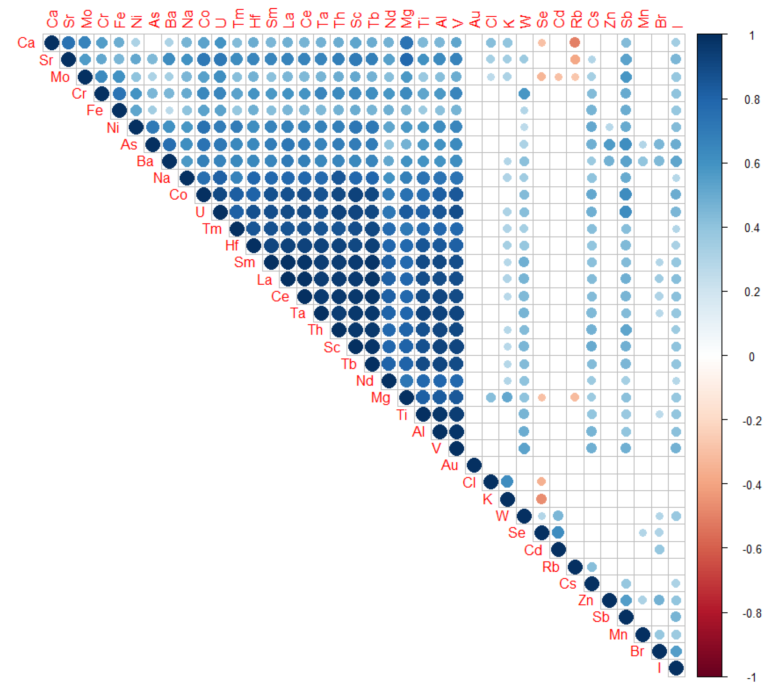
3.3. Correlations Analysis

A correlation matrix was created to assess the strength of the linear relationship between the quantities (Figure 9). Positive correlations are shown in blue and negative correlations in red. The color intensity and brand size are directly proportional to correlation coefficients. The color legend on the right shows the correlation coefficients and their corresponding color.

The correlation matrix shows a high correlation between the elements Na, Co, U, Tm, Hf, Sm, La, Ce, Ta, Th, Sc, Tb, Nd, Mg, Ti, Al, and V. A weaker positive correlation is observed for Ca, Sr, Mo, Cr, Fe, Ni, As and Ba. Negative correlation with most elements is recorded for Se, Cd, and Rb, they are positively correlated with each other. Other elements do not show significant correlations. Based on the results of the correlation matrix, clustering took place. A cluster is a group of objects whose distance is less than the distance with objects that do not belong to the cluster. Clustering was performed according to Wald’s criterion, where the principle is to minimize cluster heterogeneity according to the criterion of minimum increment of intragroup sums of deviations of objects from the center of gravity of clusters [50]. The result is a dendrogram (Figure 10). When dividing the elements into three clusters, Rb, Se, Cd, Mn, Zn, Br, Au, Cl, and K appear in the first group. The second cluster contains V, Al, Ti, Co, U, Hf, Sm, La, Ce, Ta, Th, Sc, and Tb, and the third cluster Nd, Na, Tm, Mg, Sr, Ca, Mo, Cr, Fe, Ni, As, Ba, W, Cs, Sb and I.

3.4. Contamination Factor

The Fernández and Carballeira [35] scale was used to assess contamination by the contamination factor (CF), which allows the categorization of sampling points for each element (

Table 3. Classification of elements according to the degree of contamination.

No Contamination	Suspected	Slight	Moderate
Mn	As	Al	Sm
	Cd	Cr	W
	Ni	Fe	U
	Sb	V	Tb
	Ba	Zn	Th
	Sr	Co	Sc
	Se	Mo
	Ca	Ce
	K	Na
	Mg	Cs
	Rb	Nd
	Ba	Ti
	Au	Cl

). The proposed scale includes six categories, from a contamination factor value less than 1 (no contamination) to values greater than 27 (extreme contamination). Data from moss collections in 2015 and 2016, but also from the biomonitoring campaign in 2017 (a total of 337 samples) were used to calculate background values. The concentrations of the individual elements were sorted from the smallest to the largest, and each sampling point was assigned an order for each element. The sum of the order of the individual elements was summed for each sampling point and the resulting sums were sorted again. The arithmetic mean of the first 5% points (17 values) was used as the background value.

$$\mathrm{CF}=\frac{\mathrm{Med}\left(\mathrm{concentration}\right)}{\mathrm{background}}$$

(5)

3.5. Geoaccumulation Index

The resulting values of the geoaccumulation index (Igeo) were classified by Muller [36] as shown in the following

Table 4. Degree of metal pollution in terms of seven classes.

Igeo Class	Igeo Value	Classification
0	<0	uncontaminated
1	0–1	uncontaminated to moderately contaminated
2	1–2	moderately contaminated
3	2–3	moderately to strongly contaminated
4	3–4	strongly contaminated
5	4–5	strongly to extremely contaminated
6	>5	extremely contaminated

.

The resulting Igeo element distribution is shown in the table (

Table 5. Classification of elements according to the degree of contamination.

Uncontaminated	Uncontaminated to Moderately Contaminated	Moderately Contaminated
Ni	As	Al
Mn	Cd	Fe
Se	Cr	Ce
Ca	Sb	Sm
Rb	V	W
Au	Zn	U
Br	Ba	Nd
I	Sr	Tb
	Co	Th
	Mo	Sc
	K
	Mg
	Na
	Cs
	Ba
	Cl
	Ti

).

3.6. Enrichment Factor

Due to the different scales reported in different publications [51,52] and due to the use of Sc as a normalizing element, the elements were divided into categories according to value. According to Kłos et al. [44], elements with an enrichment factor (EF) value < 1 indicate elements originating from the natural background and elements with an EF value > 1 elements affected by anthropogenic activity (

Table 6. Classification of elements according to the degree of contamination.

EF < 1		EF > 1
Mn	Sr	La
Rb	Zn	Hf
Se	Na	Fe
Au	Cs	Th
Ca	Co	Ta
Ni	Mo	Tb
Br	Tm	Sm
K	Ti	U
I	Cr	W
As	Cl
Mg	V
Ba	Nd
Cd	Ce
Sb	Al

).

3.7. Pollution Load Index

Tomlinson et al. [45] proposed a scale for evaluating the results, where zero means a perfectly clean site, a value of one means the presence of pollutants at the baseline level and concentrations above one, show a gradual deterioration in the quality of the investigated environment. Thus, it can be stated that a value of PLI < 1 defines elemental pollution close to the background value, while values of PLI > 1 indicate pollution of a given locality. Since almost the entire study area shows PLI values greater than one, a map was created to better present the results, dividing the resulting values into 6 categories (Figure 11).

4. Discussion

The findings about potential sources in terms of elemental composition, presence of potential emission sources, but also climactic and geomorphologic conditions, which allow the transmission of pollution from its source to the place of deposition, were included in the evaluation. The result of the principal components analysis is represented by the dispersion diagram of the component score (Figure 5). Based on the rules explaining the dispersion diagram, a map (Figure 12) of mutually correlated areas was created.

The points included in groups 1 and 2 are found in locations least affected by anthropogenic activity from the studied location. The sampling sites in category 3 are influenced by industrial activity and also local domestic heating and emissions from transportation, whereas the points in group 5 are not affected by emissions from industrial areas to such an extent. According to the analysis, the sites in group 6 are the most different from other sites. These points are located on the Polish side in an area of mining, engineering, and metallurgical industry. At the same time, one point is found near the town Frýdek-Místek where the metallurgical and machine-building industry is well-developed. According to the dispersion diagram, the points in category 12 are the closest to the origin and as such the most typical for the studied area; in this category, there are two points located near the village Kunčičky in the Ostrava region and close to Třinec. Metallurgical companies can be found in both of these localities.

Based on the hierarchical clustering on principal components analysis (HCPC), the sample points were divided into three clusters (Figure 8). From the clusters, we can identify areas affected by the industry, areas not significantly affected by the industry but containing a large concentration of domestic heating, and areas least affected by anthropogenic activity.

The division of elements into five factors according to the factor analysis and also the spatial distribution of the factor loadings of individual factors can be explained by the following description. Factor 1 is composed of a large number of elements (Na, Mg, Al, Sc, Ti, V, Co, Ni, As, Ba, La, Ce, Nd, Sm, Tb, Tm, Hf, Ta, Th, and U). Elements of natural origin can be influenced by the deposition from industrial sources based on the localization of the highest values of the load factor. Another source could be dust/soil particles. As described by Shetekauri et al. [28], V and Ni are the dominant elements in areas with metallurgical and mining industries. Simultaneously, the aforementioned authors attribute the natural crustal origin of elements to factor 1, which in their case also contains Ti, V, Ni, Co, As, Th, and U. Zinicovscaia et al. [27] states a combination of geogenic and anthropogenic associations in relation to Co and U as elements belonging to factor 1. Apparently, the measured results may have been affected by soil particles.

The most prominent elements in factor 2 are represented by Mn, Zn, As, and Br. Identical elements were also identified in one of the factors in the study of Olise et al. [42]. The authors note that coal impurities emitted at high temperatures contain As, Rb, As, Br, Mn, and Cr. This fact is also confirmed by other authors [53,54,55].

According to the graph of component weights (Figure 6), the element I can also be added to this group. All above-mentioned elements except for As do not show mutual correlations with other elements (Figure 9). In the calculation of all factors, manganese came out as the element least affected by anthropogenic activity. Both iodine and bromine have negative values of the geoaccumulation factor; as such, they can be considered elements of natural origin. Due to its origin, arsenic stands apart from the group as it enters the air practically only due to human activity, particularly by burning fossil fuels and wood conserved with arsenic-containing products. According to the Korzekwa et al. [29] who utilize the method of biomonitoring using mosses in Poland, another source of As besides burning fossil fuels can be represented by pesticides or products used for wood curing; this is because in their case, higher concentrations of As were found in forests or close to agricultural areas. Metallurgical companies processing copper, lead, and other metals containing arsenic in their ore are considered to be a source, too. However, the values of the contamination factor of arsenic reach the “moderate” category at maximum, and they only do so in two points (Figure 13).

One point is located in a part of Ostrava called Polanka nad Odrou where the moss was collected in a place with the following activity: Buyout and processing of alloy steel waste, processing of construction materials, selling of solid fuels and metallurgical materials, and manufacturing of asphalt mixes. The second point with its contamination factor in the “moderate” category is located in the town of Wodzisław Śląski where there are long-term issues with emissions originating from fuel burning in home boilers, undesirable technical conditions, and energetic efficiency. Other issues are also represented by the low quality of fuel burned and the burning of waste. Higher values of the contamination factor, up to the category “severe”, are displayed by four points in the case of zinc. The points described can be found in the area around the municipalities Strahovice, Pszów, Marklowice, and Żory. Significant anthropogenic sources of zinc are represented by mining, zinc, lead, and cadmium refining, steelmaking, burning of coal and other organic fuels, ore mining and processing, and utilization of zinc-containing fertilizers. Zinc is utilized to a large extent (up to 40% of production) as an anti-corrosive protective material for iron and its alloys.

According to the graph of component weights (Figure 6), Ca and Mo are more correlated with each other when compared to the pair of Cr and Fe. Based on the values of the contamination factor, calcium appears as an element included in the natural background; similarly, molybdenum belongs to the essential microelements necessary for plant development. However, Korzekwa et al. [29] states the origin of molybdenum to be the metallurgical plant. In line with this statement, higher values of the contamination factor of molybdenum correspond with the distribution of residences, pointing to anthropogenic sources such as fossil fuels burning, metallurgy, but also mining and the electrotechnical industry. In the case of Ca, the drawing of the element can occur from soil substrate according to a number of sources [42,56,57,58,59].

Higher concentrations of chromium can be found in the regions of Ostrava, Třinec, and the surrounding areas of the town Wodzisław Śląski where the mining, metallurgical, and engineering industries are well-developed. A contamination factor of the “moderate” category is also spread around smaller residencies and this reality can be caused by the burning of fossil fuels (in the form of Cr³⁺). Other sources can be represented by cement plants, communal waste incinerators, exhaust gases from automobiles with a catalyst, emissions from air-conditioning cooling towers using compounds of chromium as corrosion inhibitors, and flying asbestos from automobile brakes. High values of the contamination factor of Cr and Fe are also apparent on the north side of the Beskids Protected Landscape Area near the municipalities Řeka, Vyšní Lhoty, and Komorní Lhotka where the industry concentration is not so dense but where the massive of the Moravian–Silesian Beskids begins. Therefore, pollution is likely brought by the blowing wind from the north and its fallout and capture take place on the windy side of the massive. Iron and chromium interfere and their main sources are found in the agglomeration of Ostrava/Karviná/Frýdek Místek and in the vicinity of iron foundries. A particular affinity to absorption and accumulation of dust particles was also confirmed by Pandey et al. [60] and Olise et al. [42], who also confirms Fe as the dominant element in moss samples in the vicinity of iron and steel plants.

Factor 4 is made up of elements Se, Cd, and W. On one hand, according to the geoaccumulation factor, selenium can be considered an element of geogenic origin. This is also indicated by the scatter of its higher concentrations in the regions of the Beskids Protected Landscape Area on both the Czech and the Polish sides, the Poodří Protected Landscape Area, Oderské vrchy Natural Park, and the Cysterskie Kompozycje Krajobrazowe Rud Wielkich Protected Landscape Area. On the other hand, according to the contamination factor, selenium is “suspected of contamination”, which corresponds with the higher concentrations in the vicinity of the towns Rydyłtowy and Rybnik where the main emission sources of selenium are thermal power plants and plants of metallurgical and chemical industry. In the case of cadmium, the situation is questionable. The scatter of higher concentrations and higher levels of contamination factor of cadmium is particularly apparent in the peripheral parts of the studied area where clean locations without industry or dense settlement are found. Based on The Integrated pollution register [61], the anthropogenic emissions of cadmium are approximately eight times higher than the emissions from natural sources. One of the explanations of such scatter of concentrations is the long-distance transmission of emissions; in areas of immediate proximity of emission sources, the deposition of other substances prevails and cadmium is transported into more distant locations. Higher concentration could be caused also by transport. The points located in agricultural areas can be affected by using phosphate fertilizers with cadmium ingredients and loading waste treatment plant sewage into the fields. In the case of cadmium, it is necessary to admit an error in the analysis of the samples using the neutron activation analysis. It is evident that higher values occur only in the samples collected in the year 2016. Therefore, differences between the results from the years 2015 and 2016 can be counted on.

The differences between the elements from factor 4 and 5 and the elements from other factors are also confirmed by the results of the PCA depicted in the graph of components weights (Figure 6) where Cd, Se, Mn, and Rb show an obvious positive mutual correlation paired with a negative correlation towards Cl and K. In the case of K, intake from soil substrate can occur [56,57,58,59]. According to the PCA result, none of these elements correlates with other examined elements. This fact is confirmed by the results of the correlation matrix (Figure 9) where the elements Au, Cl, K, W, Se, Cd, Rb, Cs, Zn, Sb, Mn, Br, and I do not correlate with a greater group of other examined elements. The last element of the group, tungsten, came out to be in the category among the elements meaning contamination in all factors (CF, Igeo, EF) and as such coming from anthropogenic activity. The contamination factor of W belongs to the “moderate” and “severe” categories across the entire studied area except for peripheral areas where protected landscape areas are found. Tungsten is a part of coal and given its high density and difficult melting properties, it is widely used in a number of industrial sectors. For example, it is used in the production of lightbulb threads and W electrodes, the utilization as an ingredient in alloys to increase the hardness and mechanical and heat resistance (fast speed steel), and the production of penetration projectiles or materials for radiation shielding [62]. The contamination factor in the “moderate” category appears almost everywhere across the inhabited area. This fact can be caused by domestic heating where coal burning takes place. Higher concentrations are located in the vicinity of Třinec, Český Těšín and Cieszyna, Ostrava, Rybnik, Rydułtowy, and Wodzisław Śląski where the metallurgical industry is well-developed.

Factor 5 is made of elements Cl and K. The highest values appeared particularly in agricultural areas. Based on the result of Igeo, CF, and EF, potassium is a part of the natural background; it is a biogenic element and therefore, a vegetal origin can be expected. For instance, Olise et al. [42] identified crustal/soil dust as a source. In the case of CF, chlorine is classified into the slight contaminated category. By comparing the distribution of its concentrations with the distribution of the corresponding CF values, locations where high values are a part of the natural background are eliminated (Figure 14).

Most of the locations with higher CF values are found in the vicinity of agricultural areas and an influence through the use of potassium fertilizers, whose basic component is potassium chloride (KCl) or potassium sulfate (K₂SO₄), can be assumed. Higher values in the areas surrounding Ostrava, Frýdek Místek, and the Polish city Skoczów can originate from chlorine and hydrogen chloride leaks from the industry, specifically from their production and processing, the burning of chloride-containing fuels such as coal, or the leakage of hydrochloric acid during steel processing.

Regarding the rate of excessive of the concentration of heavy metals in the natural environment calculated using the Tomlinson Pollution Load Index (PLI) based on the division of values into categories greater or less than one, expressing if given concentrations in a given location are nearing the value of the background or indicating pollution, the results identified nearly the entire studied area (except for six points in the southern mountainous part) as affected by anthropogenic activity. Similar results were also reached by Shirani et al. [13]. For that reason, a map with PLI values divided into six categories (Figure 11) was created. Higher PLI values correspond with the distribution of industrial centers on both the Czech and the Polish side. High values are also located to the west and south-west of the cities Frýdek-Místek and Paskov, reaching into the Poodří Protected Landscape Area where higher concentration of industry is not found. This reality can be caused by the north-east drift from industrial areas or domestic heating together with transportation emissions. In this location, an airport can also be found. However, none of the performed statistical analyses determined the link between higher concentrations of individual heavy metals and the vicinity of the airport. Moderately elevated PLI values are observed on the north windy side of the Beskids. Except for typical industrial areas in the studied location, high PLI values are also found in the area surrounding Dolní Benešov where the engineering industry and a foundry are located. A high index also appears in the north part of the Opava region in the Sudice-Třebom promontory. Despite the absence of heavy industry, high concentrations of a number of elements (As, Br, Mn, Zn, Ca, Cr, Fe, Mo, Cd, W, Sc, and Cl) can be found there. This fact can be affected by the surface gypsum mine located in the land registry of the municipality Koběřice where the subsequent processing of natural gypsum also takes place. Another influence in this area can come from domestic heating, particularly in the town Třebom where according to the results of the 2011 census of persons, houses, and flats [63], heating with solid fuels, particularly with coal, coke, or coal briquettes, prevails. Additionally, transmission of emissions to this area from the Polish side probably takes place.

5. Conclusions

During the years 2015, 2016, 99 samples of moss were collected, the results of which were processed as part of the presented work. After eliminating unsuitable samples, 93 samples were included in the analyses. The samples were analyzed using the instrumental neutron activation analysis. The result was represented by 38 variables, the chemical elements.

A partial goal of this work was to evaluate the measured data and determine if the elements contained in the samples were of natural or anthropogenic origin. To reach this goal, multi-criteria analysis of data was used. Hierarchical clustering on principal components and factor analysis were conducted. Through the principal component analysis, locations most typical for the studied area were determined; these were the locations in the immediate vicinity of metallurgical plants. From the results of this partial goal, it can be assumed that the dominant polluter of the area of interest likely is the metallurgical industry. By hierarchical clustering, the area was divided, according to the type of pollution, into three groups composed of an industry-influenced group, a group with prevailing emissions from domestic heating and also industrial emissions from long-distance transmission, and a so-called clean group.

The distinction between elements with their concentrations near the natural background and elements which can indicate pollution was performed using a number of factors, namely the contamination, geoaccumulation, and enrichment factor and the pollution load index. An intersection of a set of elements Sm, W, U, Tb, and Th, which were determined to be the elements causing pollution and whose concentrations do not near the natural background of the studied locations, took place in all factors. The elements are emitted among others by the metallurgical industry. Sm and Th are applied in a number of chemical industries. Tb is used moreover by electronic industry. W and U are substantial compound of coal. High concentrations in samples coming from areas with no local sources of pollution can be associated with a climactic standpoint, particularly for the prevailing direction of the wind, and long-distance transmission of pollute.

Moss sampling in the study was carried out in an exceptional dense network of sampling sites. Based on the results of the paper, it is possible to propose a dense sampling of the entire region of the Czech Republic as biomonitoring with the use of mosses gives us the ability to detect regional sources of air pollution in a sufficiently dense network yet at acceptable costs.

References

1. Mulgrew, A.; Williams, P. Biomonitoring of Air Quality Using Plants; Air Hygiene Report; WHO Collab. Centre for Air Quality Management and Air Pollution Control: Berlin, Germany, 2000. [Google Scholar]
2. Satsangi, G.; Yadav, S.; Pipal, A.; Kumbhar, N. Characteristics of trace metals in fine (PM2.5) and inhalable (PM10) particles and its health risk assessment along with in-silico approach in indoor environment of India. Atmos. Environ. 2014, 92, 384–393. [Google Scholar] [CrossRef]
3. Sarti, E.; Pasti, L.; Rossi, M.; Ascanelli, M.; Pagnoni, A.; Trombini, M.; Remelli, M. The composition of PM1 and PM2.5 samples, metals and their water soluble fractions in the Bologna area (Italy). Atmos. Pollut. Res. 2015, 6. [Google Scholar] [CrossRef] [Green Version]
4. European Environment Information and Observation Network (Eionet). European Environment Agency. Available online: https://www.eea.europa.eu/ (accessed on 26 May 2020).
5. Cherry Hill Mortgage Investment Corp. ISKO: Informace o úrovni Znečištění Ovzduší ve Smyslu Zákona o Ochraně Ovzduší. Available online: http://portal.chmi.cz/ (accessed on 11 March 2019).
6. Cherry Hill Mortgage Investment Corp. Register of Emissions and Air Polution Sources (REZZO). Available online: http://portal.chmi.cz/files/portal/docs/uoco/oez/embil/11embil/rezzo1_4/rezzo1_4_CZ.html (accessed on 26 May 2020).
7. Krakovská, A.S. Analýza Prostorových Dat z Biomonitoringu v Průmyslových Oblastech. Ph.D. Thesis, VSB–Technical University of Ostrava, Ostrava, Czech Republic, 2020. [Google Scholar]
8. UC Centre for Ecology and Hydrology. ICP Vegetation. Available online: https://icpvegetation.ceh.ac.uk/ (accessed on 26 May 2020).
9. Rodrigues, L.A.; Daunis-i Estadella, P.; Figueras, G.; Henestrosa, S. Compositional Data Analysis: Theory and Applications; John Wiley & Sons: Hoboken, NJ, USA, 2011; pp. 235–254. [Google Scholar] [CrossRef]
10. Eaton, M. Multivariate Statistics: A Vector Space Approach; Lecture Notes-Monograph Series; Institute of Mathematical Statistics: Hoboken, NJ, USA, 2007. [Google Scholar]
11. Aitchison, J. The Statistical Analysis of Compositional Data; Chapman & Hall, Ltd.: GBR, Australia, 1986. [Google Scholar]
12. Hron, K. Elementy Statistické Analýzy Kompozičních Dat in Informační Bulletin České Statistické Společnosti; Praha, Czech Republic, 2010; Volume 3, Available online: https://www.statspol.cz/oldstat/bulletiny/ib-2010-3.pdf (accessed on 25 October 2020).
13. Shirani, M.; Afzali, K.; Jahan, S.; Strezov, V.; Soleimani-Sardo, M. Pollution and contamination assessment of heavy metals in the sediments of Jazmurian playa in southeast Iran. Sci. Rep. 2020, 10. [Google Scholar] [CrossRef]
14. Jiang, H.H.; Cai, L.; Wen, H.H.; Luo, J. Characterizing pollution and source identification of heavy metals in soils using geochemical baseline and PMF approach. Sci. Rep. 2020, 10. [Google Scholar] [CrossRef] [PubMed] [Green Version]
15. Betsou, C.; Tsakiri, E.; Kazakis, N.; Vasilev, A.; Frontasyeva, M.; Ioannidou, A. Atmospheric deposition of trace elements in Greece using moss Hypnum cupressiforme Hedw. as biomonitors. J. Radioanal. Nucl. Chem. 2019, 320, 597–608. [Google Scholar] [CrossRef]
16. Koroleva, Y.; Napreenko, M.; Baymuratov, R.; Schefer, R. Bryophytes as a bioindicator for atmospheric deposition in different coastal habitats (a case study in the Russian sector of the Curonian Spit, South-Eastern Baltic). Int. J. Environ. Stud. 2020, 77, 152–162. [Google Scholar] [CrossRef]
17. Demková, L.; Árvay, J.; Bobulska, L.; Hauptvogl, M.; Hrstková, M. Open mining pits and heaps of waste material as the source of undesirable substances: Biomonitoring of air and soil pollution in former mining area (Dubnik, Slovakia). Environ. Sci. Pollut. Res. 2019, 26. [Google Scholar] [CrossRef] [PubMed]
18. Aničić Urošević, M.; Frontasyeva, M.; Tomasevic, M.; Popovic, A. Assessment of Atmospheric Deposition of Heavy Metals and Other Elements in Belgrade Using the Moss Biomonitoring Technique and Neutron Activation Analysis. Environ. Monit. Assess. 2007, 129, 207–219. [Google Scholar] [CrossRef] [PubMed]
19. Vergel, K.; Zinicovscaia, I.; Yushin, N.; Frontasyeva, M. Heavy Metal Atmospheric Deposition Study in Moscow Region, Russia. Bull. Environ. Contam. Toxicol. 2019, 103. [Google Scholar] [CrossRef]
20. Thieme, N. R generation. Significance 2018, 15, 14–19. [Google Scholar] [CrossRef]
21. Templ, M.; Hron, K.; Filzmoser, P. robCompositions: An R-Package for Robust Statistical Analysis of Compositional Data. In Compositional Data Analysis: Theory and Applications; John Wiley and Sons, Ltd.: Chichester, UK, 2011; pp. 341–345. [Google Scholar]
22. Lê, S.; Josse, J.; Husson, F. FactoMineR: An R Package for Multivariate Analysis. J. Stat. Softw. Artic. 2008, 25, 1–18. [Google Scholar] [CrossRef] [Green Version]
23. Wei, T.; Simko, V. R Package “Corrplot”: Visualization of a Correlation Matrix; Version 0.84; 2017; Available online: https://github.com/taiyun/corrplot/ (accessed on 26 May 2020).
24. StatSoft CR s.r.o. TIBCO Statistica. Available online: http://www.statsoft.cz/ (accessed on 26 May 2020).
25. Barandovski, L.; Frontasyeva, M.; Stafilov, T.; Sajn, R.; Ostrovnaya, T. Multi-element atmospheric deposition in Macedonia studied by the moss biomonitoring technique. Environ. Sci. Pollut. Res. 2015. [Google Scholar] [CrossRef] [PubMed]
26. Bajraktari, N.; Morina, I.; Demaku, S. Assessing the Presence of Heavy Metals in the Area of Glloogoc (Kosovo) by Using Mosses as a Bioindicator for Heavy Metals. J. Ecol. Eng. 2019, 20, 135–140. [Google Scholar] [CrossRef]
27. Zinicovscaia, I.; Aničić Urošević, M.; Vergel, K.; Vieru, E.; Frontasyeva, M.; Povar, I.; Duca, G. Active Moss Biomonitoring of Trace Elements Air Pollution in Chisinau, Republic of Moldova. Ecol. Chem. Eng. 2018, 25, 361–372. [Google Scholar] [CrossRef] [Green Version]
28. Shetekauri, S.; Chaligava, O.; Shetekauri, T.; Kvlividze, A.; Kalabegishvili, T.; Kirkesali, E.; Frontasyeva, M.; Chepurchenko, O.; Tselmovich, V. Biomonitoring Air Pollution Using Moss in Georgia. Pol. J. Environ. Stud. 2018, 27. [Google Scholar] [CrossRef]
29. Korzekwa, S.; Frontasyeva, M. Air Pollution Studies in Opole Region, Poland, Using the Moss Biomonitoring and INAA. Am. Inst. Phys. 2007, 958, 230–231. [Google Scholar] [CrossRef]
30. Ermakova, E.; Frontasyeva, M.; Pavlov, S.; Povtoreiko, E.; Steinnes, E.; Cheremisina, Y. Air Pollution Studies in Central Russia (Tver and Yaroslavl Regions) Using the Moss Biomonitoring Technique and Neutron Activation Analysis. J. Atmos. Chem. 2004, 49, 549–561. [Google Scholar] [CrossRef] [Green Version]
31. Haruštiaková, D.; Jarkovský, J.; Littnerová, S.; Dušek, L. Vícerozměrné Statistické Metody v Biologii; Akademické nakladatelství CERM, s.r.o.: Brno, Czech Republic, 2012. [Google Scholar]
32. Hebák, P. Vícerozměrné Statistické Metody; Informatorium: Praha, Czech Republic, 2007. [Google Scholar]
33. Legendre, P.; Legendre, L. Numerical Ecology, 3rd ed.; Elsevier: Amsterdam, The Netherlands, 2012. [Google Scholar]
34. Håkanson, L. An Ecological Risk Index for Aquatic Pollution Control—A Sedimentological Approach. Water Res. 1980, 14, 975–1001. [Google Scholar] [CrossRef]
35. Fernández, J.; Rey, A.; Carballeira, A. An extended study of heavy metal deposition in Galicia (NW Spain) based on moss analysis. Sci. Total Environ. 2000, 254, 31–44. [Google Scholar] [CrossRef]
36. Muller, G. Index of Geoaccumulation in Sediments of the Rhine River. Geojournal 1969, 2, 109–118. [Google Scholar]
37. Turekian, K.; Wedepohl, K. Distribution of the Elements in Some Major Units of the Earth’s Crust. Geol. Soc. Am. Bull. 1961, 72. [Google Scholar] [CrossRef]
38. Covelli, S.; Fontolan, G. Application of a normalization procedure in determining regional geochemical baselines. Environ. Geol. 1997, 30, 34–45. [Google Scholar] [CrossRef]
39. Sinex, S.; Helz, G. Regional geochemistry of trace elements in Chesapeake Bay sediments. Environ. Geol. 1981, 3, 315–323. [Google Scholar] [CrossRef]
40. Rubio, B.; Nombela, M.; Vilas, F. Geochemistry of Major and Trace Elements in Sediments of the Ria de Vigo (NW Spain): An Assessment of Metal Pollution. Mar. Pollut. Bull. 2000, 40, 968–980. [Google Scholar] [CrossRef]
41. Ackermann, F. A procedure for correcting the grain size effect in heavy metal analyses of estuarine and coastal sediments. Environ. Technol. Lett. 2008, 1. [Google Scholar] [CrossRef]
42. Olise, F.; Lasun Tunde, O.; Olajire, M.; Owoade, O.; Oloyede, F.; Fawole, O.G.; Ezeh, G. Biomonitoring of environmental pollution in the vicinity of iron and steel smelters in southwestern Nigeria using transplanted lichens and mosses. Environ. Monit. Assess. 2019, 191. [Google Scholar] [CrossRef]
43. Rotter, P.; Šrámek, V.; Vácha, R.; Borůvka, L.; Fadrhonsová, V.; Sáňka, M.; Drábek, O.; Vortelová, L. Rizikové prvky v lesních půdách: review. ZpráVy Lesn. VýZkumu 2013, 58, 17–27. [Google Scholar]
44. Kłos, A.; Rajfur, M.; Wacławek, M.; Wacławek, M. Application of enrichment factor (EF) to the interpretation of results from the biomonitoring studies. Ecol. Chem. Eng. 2011, 18, 171–183. [Google Scholar]
45. Tomlinson, D.; Wilson, J.; Harris, C.; Jeffrey, D. Problems in Assessment of Heavy Metals in Estuaries and the Formation of Pollution Index. HelgoläNder Meeresunters. 1980, 33, 566–575. [Google Scholar] [CrossRef] [Green Version]
46. Salo, H.; Bućko, M.; Vaahtovuo, E.; Limo, J.; Mäkinen, J.; Pesonen, L. Biomonitoring of air pollution in SW Finland by magnetic and chemical measurements of moss bags and lichens. J. Geochem. Explor. 2012, 115, 69–81. [Google Scholar] [CrossRef]
47. Angulo, E. The Tomlinson Pollution Load Index applied to heavy metal, ’Mussel-Watch’ data: A useful index to assess coastal pollution. Sci. Total Environ. 1996, 187, 19–56. [Google Scholar] [CrossRef]
48. Aitchison, J.; Greenacre, M. Biplots of Compositional Data. J. R. Stat. Soc. Ser. 2002, 51, 375–392. [Google Scholar] [CrossRef] [Green Version]
49. Cartell, R. The Scree Test for the Number of Factors. Multivar. Behav. Res. 1966, 1, 245–276. [Google Scholar] [CrossRef] [PubMed]
50. Meloun, M. Vícerozměrná Analýza Dat Metodou Hlavních Komponent a Shluků; Analýza Dat 2015; Celostátní Seminář a Workshop: Pardubice, Czech Republic, 2015; pp. 25–42. [Google Scholar]
51. Barbieri, M. The Importance of Enrichment Factor (EF) and Geoaccumulation Index (Igeo) to Evaluate the Soil Contamination. J. Geol. Geophys. 2016, 5. [Google Scholar] [CrossRef]
52. Nowrouzi, M.; Pourkhabbaz, A. Application of geoaccumulation index and enrichment factor for assessing metal contamination in the sediments of Hara Biosphere Reserve, Iran. Chem. Speciat. Bioavailab. 2014, 26. [Google Scholar] [CrossRef] [Green Version]
53. Pant, P.; Harrison, R. Critical Review of Receptor Modelling for Particulate Matter: A Case Study of India. Atmos. Environ. 2012, 49, 1–12. [Google Scholar] [CrossRef]
54. Fawole, O.; Owoade, O.; Hopke, P.; Olise, F.; Lasun Tunde, O.; Olaniyi, B.; Jegede, O.; Ayoola, M.; Bashiru, M. Chemical compositions and source identification of particulate matter (PM2.5 and PM2.5–10) from a scrap iron and steel smelting industry along the Ife–Ibadan highway, Nigeria. Atmos. Pollut. Res. 2015, 6, 107–119. [Google Scholar] [CrossRef]
55. Kara, M.; Hopke, P.; Dumanoglu, Y.; Altiok, H.; Elbir, T.; Odabasi, M.; Bayram, A. Characterization of PM Using Multiple Site Data in a Heavily Industrialized Region of Turkey. Aerosol Air Qual. Res. 2015, 15, 11–27. [Google Scholar] [CrossRef]
56. Bates, J.; Farmer, A. Bryophytes and Lichens in a Changing Environment; Oxford University Press: New York, NY, USA, 1992. [Google Scholar]
57. Wells, J.; Boddy, L. Phosphorous translocation by saprotrophic basidiomycete cord systems on the floor of a mixed deciduous woodland. Mycol. Res. 1995, 99, 977–980. [Google Scholar] [CrossRef]
58. Brown, D.; Brumelis, G. A biomonitoring method using the cellular distribution of metals in moss. Sci. Total Environ. 1996, 187, 153–161. [Google Scholar] [CrossRef]
59. Brumelis, G.; Brown, D. Movement of Metals to New Growing Tissue in the Moss Hylocomium splendens (Hedw.) BSG. Ann. Bot. 1997, 79. [Google Scholar] [CrossRef] [Green Version]
60. Pandey, V.; Upreti, D.; Pathak, R.; Pal, A. Heavy Metal Accumulation in Lichens from the Hetauda Industrial Area Narayani Zone Makwanpur District, Nepal. Environ. Monit. Assess. 2002, 73, 221–228. [Google Scholar] [CrossRef] [PubMed]
61. Praha: Ministerstvo životního Prostředí, CENIA. Integrovaný Registr Znečišťování životního Prostředí. Available online: https://www.irz.cz/ (accessed on 26 May 2020).
62. Greenwood, N.N.; Earnshaw, A. Chemie Prvků; Informatorium: Praha, Czech Republic, 1993. [Google Scholar]
63. Český Statistický úřad (ČSÚ). Český Statistický úřad. Available online: https://www.czso.cz/ (accessed on 26 May 2020).
Figure 1. Annual mean concentration of PM10 [4].
Atmosphere 11 01237 g001
Figure 2. Annual mean concentration of PM10 in the Czech Republic [5].
Atmosphere 11 01237 g002
Figure 3. Map of sampling area.
Atmosphere 11 01237 g003
Figure 4. Map of sampling sites.
Atmosphere 11 01237 g004
Figure 5. Scatterplot of the component score of individual sampling sites.
Atmosphere 11 01237 g005
Figure 6. Plot Components Weigh of individual elements.
Atmosphere 11 01237 g006
Figure 7. Graph of main components with clusters.
Atmosphere 11 01237 g007
Figure 8. The result of hierarchical clustering on three components.
Atmosphere 11 01237 g008
Figure 9. Correlation matrix.
Atmosphere 11 01237 g009
Figure 10. Hierarchical clustering based on a correlation matrix.
Atmosphere 11 01237 g010
Figure 11. Pollution load index.
Atmosphere 11 01237 g011
Figure 12. The result of the principal components analysis.
Atmosphere 11 01237 g012
Figure 13. The distribution of values of the contamination factor for As.
Atmosphere 11 01237 g013
Figure 14. The distribution of concentrations of Cl and the values of the contamination factor for Cl.
Atmosphere 11 01237 g014