Analysis of Weather Patterns Related to Wintertime Particulate Matter Concentration in Seoul and a CMIP6-Based Air Quality Projection

Abstract

This study analyzes the relationship between various atmospheric fields and the observed PM₁₀ concentrations in the Seoul metropolitan area, South Korea, during the winters of the 2001–2014 period to find suitable atmospheric indices for predicting high PM₁₀ episodes in the region. The analysis shows that PM₁₀ concentration in the metropolitan area is mainly affected by the intensity of horizontal ventilation and the 500 hPa high-pressure system over the Korean peninsula. The modified Korea particulate matter index (MKPI) is proposed based on a 10 m wind speed for surface ventilation and 500 hPa zonal wind for the intensity of a 500 hPa high-pressure system over the Korean peninsula. It is found that a positive MKPI value is closely correlated with the occurrence of high PM₁₀ concentration episodes, and hence, can be used as a predictor for high PM₁₀ episodes in the area. A future projection of the MKPI using two three-member general circulation model (GCM) ensembles with four shared socioeconomic pathway (SSP) scenarios in Coupled Model Intercomparison Project Phase 6 (CMIP6) shows that positive MKPI events and high PM₁₀ episodes are expected to increase by 5.4−16.4% depending on the SSP scenarios in the 2081−2100 period from the present-day period of 1995−2014.

1. Introduction

Industrialization and high population density have caused severe air pollution in urbanized areas worldwide [1,2]. Exposure to fine particulate matter poses a public health risk as a potential cause for heart and respiratory diseases and, thereby, increased mortality [1,3,4,5]. The World Health Organization (WHO) has recognized the damage caused by particulate matter in the air and set the PM₁₀ limits at 50 μg/m³ for a 24-h period and an annual average of 20 μg/m³ [6].

Particulate matter of ≤10 μm in size (PM₁₀) in the atmosphere contains primary products generated during the combustion of fossil fuels, forest fires, automobiles, and industrial facilities. PM₁₀ concentrations are affected not only by local emissions but also by meteorological fields such as the upstream wind trajectory, boundary layer, wind gusts, sea-level pressure, and precipitation.

In 2005, the South Korean government set the annual average concentration limit for PM₁₀ in metropolitan areas at 40 µg/m³, which is higher than the corresponding WHO guideline, and implemented the Second Basic Plan for Atmospheric Environment Regulation (2013) for 10 years including a strict policy for the reduction of air pollutants in major cities such as Seoul, Busan, Daegu, Daejeon, and Gwangju, where about 50% of the country’s population lives [7]. As a result, the concentration of PM₁₀ continuously decreased every year; however, currently, the PM₁₀ level remains above the target concentration of 40 µg/m³ [8,9]. In addition, PM₁₀ is reported to be two to three times higher than in the major cities of the Organization for Economic Cooperation and Development (OECD) [10].

The Korean peninsula is affected by the transboundary transports of pollutants generated by industrial regions in China [8,10,11,12]. It has been noted that secondary particles, such as sulfate and nitrate, travel long distances. These secondary particles from China’s inland and industrial facilities (Beijing and Tianjin) can reach the Korean peninsula by prevailing westerlies [8,13,14]. High PM₁₀ episodes occur frequently in the winter season [8,10,11,12]. In the winter, elevated emissions come from primary sources of heating, frequent inversion temperatures, lower boundary layer heights, and stagnant atmospheric conditions. Thin boundary layers and stagnant conditions due to high pressure over the Asian continent provide favorable conditions for accumulating PM and secondary air pollutants [10]. The Korean peninsula has experienced frequent atmospheric stagnation due to the influence of continental high pressure [8,13,14]. Stagnated air conditions can cause harmful air quality by adapting and sustaining fine particles in the atmosphere [8,15,16]. Hong et al. [5] found that the majority of high PM_2.5 concentration events in 74 major cities in China occurred during atmospheric stagnation. About 72% and 90% of the events in which PM_2.5 concentrations were over 150 μg/m³ and 250 μg/m³, respectively, occurred during atmospheric stagnation.

Based on this, Lee et al. [10] analyzed the meteorological characteristics of high-concentration PM₁₀ episodes in the Seoul metropolitan area during the winter (December–January–February (DJF)) and developed the Korean particulate matter index (KPI) based on atmospheric variables including 850 hPa meridional winds, 500 hPa geopotential heights, and zonal winds. Based on the KPI, two future scenarios in terms of the representative concentration pathways (RCP) RCP4.5 and RCP8.5 of the Coupled Model Intercomparison Project Phase 5 (CMIP5) predicted that the frequency of atmospheric patterns favorable to high concentrations would increase significantly by the end of the 21st century.

According to Lee et al. [8], weak winds around the Korean peninsula are also favorable for PM₁₀ accumulation. Zou et al. [17] revealed that the pressure levels 1000 hPa horizontal ventilation and 925−1000 hPa vertical ventilation play a very important role in the occurrence of extreme winter haze episodes in the East China Plain (ECP), which was indexed using a vertical gradient of potential temperature and surface wind speed. Kim et al. [14] confirmed that the ventilation of the near-surface atmosphere used in the ECP was related to PM₁₀ in South Korea, and as a result, horizontal ventilation was significantly related to PM₁₀ in January. Kim et al. [14] analyzed the differences in the correlations of PM₁₀ with vertical and horizontal ventilation in the lower atmosphere.

This study examines the relationship between selected atmospheric variables and PM₁₀ concentration over the Seoul metropolitan area. Based on the examination, we attempt to develop an index suitable for predicting PM₁₀ concentration in the South Korean metropolitan area with an emphasis on high-concentration events. We also apply the newly developed index and use it to project the impacts of climate change on the occurrence of high PM₁₀ episodes using the climate scenarios in the Coupled Model Intercomparison Project Phase 6 (CMIP6) and compare the projection against the projections in previous studies such as [10,18].

The rest of the paper is organized as follows: Section 2 describes the model and presents the observations on the PM₁₀ data used in this study. The main results, including the atmospheric index and future projections, are presented in Section 3. Section 4 summarizes the study.

2. Experiments

2.1. Station PM₁₀ Data and Reanalysis Data

This study employed the hourly PM₁₀ mass concentrations measured at 25 air-quality-monitoring sites in Seoul during the 2001–2014 period. The collected hourly data were converted into daily average values. The representative PM₁₀ concentration in Seoul was defined as the daily average value of the 25 stations. High PM₁₀ episodes were defined as the events in which the daily mean PM₁₀ concentration exceeds 100 µg/m³ in accordance with previous studies [8,10,12,14,19]. High PM₁₀ episodes may have been caused by either yellow dust, anthropogenic sources, or both [8,12,19,20]. This study focused only on anthropogenic PM₁₀ episodes and excluded the yellow dust cases caused by natural sources. The 146 days in which yellow dust was identified by the Korea Meteorological Administration (KMA) were excluded from the analysis. Meteorological data for the PM₁₀-related characterization analysis including surface wind speed, zonal and meridional winds (u and v), and geopotential height and potential temperature were obtained from the ERA-Interim database with a longitude–latitude resolution of 0.75° × 0.75°. This study used anomalies obtained by removing the seasonal climate average (during the 1981–2010 period) to analyze the synoptic characteristics related to PM₁₀.

2.2. Models

Climate models are constantly being updated, with different modeling groups around the world incorporating finer spatial resolution, improved parameterizations for cloud microphysical processes, and the inclusion of additional processes and biogeochemical cycles. These modeling groups, which are part of CMIP, coordinate their updates according to the Intergovernmental Panel on Climate Change’s (IPCC) assessment report schedule and release climate models. In the lead up to the IPCC, the modeling community has developed future scenarios for assessment reports.

The 2013 IPCC AR5 featured climate models from CMIP5 and future radiative forcing by greenhouse gases (GHGs) in terms of representative concentration pathways (e.g., RCP2.5, RCP4.5, RCP6.0, RCP8.5, etc.). The RCP assumes that radiative forcing will increase until the end of the 21st century and stabilize at 2.5/4.5/6.0/8.5 W/m², respectively. The upcoming 2021 IPCC Sixth Assessment Report (AR6) will feature new state-of-the-art CMIP6 models and shared socioeconomic pathways (SSPs). CMIP6 generates four high-priority scenarios (SSP1-2.6, SSP2-4.5, SSP3-7.0, and SSP5-8.5) for the IPCC AR6. The SSPs assume that radiative forcing will increase until the end of the 21st century and stabilize at 2.5/4.5/7.0/8.5 W/m², respectively. These updated SSPs include parameters such as the rate of technological development, economic growth, education, urbanization, and population. These SSPs look at the different ways in which the world might evolve in the absence of climate policies and how different levels of climate change mitigation could be achieved when the mitigation targets of RCPs are combined with SSPs

We used two climate models that are participating in the CMIP6: the Korea Meteorological Administration’s (KMA) Advanced Community Earth System (K-ACE) model and the United Kingdom Earth System Model Version 1 (UKESM1). Each provides three ensemble members. Both models are based on the physical climate model HadGEM3-GC3.1 [21,22]. Both models employ the same modules for the atmosphere, land, and sea ice components. The component models of HadGEM3-GC3.1 are the unified model (UM) for the atmosphere, the Los Alamos sea ice model (CICE) for sea ice, and the joint UK land environment simulator (JULES) model for land surface processes. The horizontal resolutions are N96 (~135 km, 1.875° (latitude) × 1.31° (longitude)) and there are 85 vertical layers within the atmosphere. The two climate models use the nucleus for European modeling of the ocean (NEMO) for UKESM1 and the modular ocean model (MOM) of Geophysical Fluid Dynamics Laboratory (GFDL) for K-ACE. Details of the components of the two Earth system models and the coupling process are described in K-ACE [23] and UKESM1 [24], respectively.

For the analysis of weather conditions pertaining to the PM₁₀ concentrations in Seoul, the 1981–2014 period in the historical simulations (1860–2014) was used. For future projections, SSPs including SSP1-2.6, SSP2-4.5, SSP3-7.0, and SSP5-8.5 were utilized. The prediction periods were set for the near-term future (2031–2050) and long-term future (2081–2100) during the SSP scenario of the 2014–2100 period. The reanalysis data were linearly interpolated to the N96 resolution of the CMIP6.

2.3. Atmosphere Pattern Index

Table 1. The indices and definitions of the 6 indices used in the study.

Reference	Index	Defined Area
Lee et al. [10]	500 hPa u-wind index (U500I)	(45° N–55° N, 110° E–140° E) –(30° N–40° N, 110° E–140° E)
	850 hPa v-wind index (V850I)	25° N–40° N, 115° E–135° E
	500 hPa geopotential index (Z500I)	35° N–50° N, 110° E–140° E
Kim et al. [14]	Potential air temperature gradient index (ATGI)	33° N–38° N, 125° E–130° E
	1000 hPa wind speed index (WS1000I)	33° N–38° N, 125° E–130° E
This paper	10 m wind speed index (WSSFCI)	25° N–40° N, 115° E–135° E
	500 hPa u-wind index (U500I)	(45° N–55° N, 110° E–140° E)–(30° N–40° N, 110° E–140° E)

presents the indices defined in this study with those of [10,14]. For the atmospheric circulation anomalies during the winter season, the high PM₁₀ cases found in [10] are characterized by persistent high-pressure anomalies at 500 hPa (Z500) over the Korean peninsula, weakened northwesterly anomalies at 850 hPa (V850), and a northward shift of the meridional wind anomalies at 500 hPa (U500) [10]. Lee et al. [10] developed KPI (Equation (5)) in terms of the mean (Equation (4)) of the normalized U500, Z500, and V850 as in Equations (1), (2) and (3), respectively.

$$\mathrm{U}500{\mathrm{I}}_{\mathrm{i}}^{\mathrm{j}}=\left(\mathrm{U}{500}_{\mathrm{i}}^{\mathrm{j}}-\mathrm{U}{500}_{\mathrm{mean}}^{\mathrm{j}}\right)/\mathrm{U}{500}_{\mathrm{std}}^{\mathrm{j}}$$

(1)

$$\mathrm{Z}500{\mathrm{I}}_{\mathrm{i}}^{\mathrm{j}}=(\mathrm{Z}{500}_{\mathrm{i}}^{\mathrm{j}}-\mathrm{Z}{500}_{\mathrm{mean}}^{\mathrm{j}})/\mathrm{Z}{500}_{\mathrm{std}}^{\mathrm{j}}$$

(2)

$$\mathrm{V}850{\mathrm{I}}_{\mathrm{i}}^{\mathrm{j}}=(\mathrm{V}{8500}_{\mathrm{i}}^{\mathrm{j}}-\mathrm{V}{850}_{\mathrm{mean}}^{\mathrm{j}})/\mathrm{V}{850}_{\mathrm{std}}^{\mathrm{j}}$$

(3)

$${\mathrm{Index}\mathrm{Mean}}_{\mathrm{i}}=\frac{\mathrm{U}500{\mathrm{I}}_{\mathrm{i}}^{\mathrm{Area}\mathrm{average}}+\mathrm{Z}500{\mathrm{I}}_{\mathrm{i}}^{\mathrm{Area}\mathrm{average}}+\mathrm{V}850{\mathrm{I}}_{\mathrm{i}}^{\mathrm{Area}\mathrm{average}}}{3}$$

(4)

$${\mathrm{KPI}}_{\mathrm{i}}=\frac{{\mathrm{Index}\mathrm{Mean}}_{\mathrm{i}}}{{\mathrm{Index}\mathrm{Mean}}_{\mathrm{std}}}$$

(5)

The subscripts ‘i’ and ‘j’ denote the time steps and spatial locations (i.e., grid points), respectively. The subscripts ‘mean’ and ‘std’ represent the mean and temporal standard deviations over the reference period (1981−2010). The superscript ‘Area average’ indicates the mean over the region defined in Table 1. Note that the area for which the averages are calculated varies according to the variables.

Kim et al. [14] used a potential air temperature gradient index (ATGI) and 1000 hPa wind speed index (WS1000I) to represent the vertical ventilation effect and horizontal ventilation effect, respectively. ATGI was defined as the normalized vertical potential air temperature gradient between 925 hPa and 1000 hPa as in Equation (6). WS1000I was defined as the normalized horizontal wind speed of 1000 hPa as in Equation (7). The two ventilation indices were calculated over the area of South Korea (33–38° N, 125–130° E).

$${\mathrm{ATGI}}_{\mathrm{i}}^{\mathrm{j}}=\left({\mathrm{ATG}}_{\mathrm{i}}^{\mathrm{j}}-{\mathrm{ATG}}_{\mathrm{mean}}^{\mathrm{j}}\right)/{\mathrm{ATG}}_{\mathrm{std}}^{\mathrm{j}}$$

(6)

$$\mathrm{WS}1000{\mathrm{I}}_{\mathrm{i}}^{\mathrm{j}}=(\mathrm{WS}{1000}_{\mathrm{i}}^{\mathrm{j}}-\mathrm{WS}{1000}_{\mathrm{mean}}^{\mathrm{j}})/\mathrm{WS}{1000}_{\mathrm{std}}^{\mathrm{j}}$$

(7)

We modified the Korea particulate index (MKPI), which improves the KPI index of [10], developed using the 500 hPa u-wind index (U500I) and negative surface wind speed index (NWSSFCI) (Equations (8)–(12)). As the positive value of the MKPI increases, the pressure at 500 hPa increases over the Korean peninsula and the surface horizontal ventilation effects decrease, implying that the stagnant atmospheric condition is strengthened.

In addition, we also defined the negative surface wind speed index (NWSSFCI), which was obtained by multiplying the negative value of the surface wind speed index (WSSFCI) (Equation (9)). NWSSFC is used instead of the WSSFCI because a positive NWSSFCI corresponds to stagnant wind conditions that are closely correlated with high PM₁₀ concentrations. Thus, using the NWSSFCI is more intuitive than using the WSSFCI in relating the wind indices to the MKPI.

$$\mathrm{U}500{\mathrm{I}}_{\mathrm{i}}^{\mathrm{j}}=\left(\mathrm{U}{500}_{\mathrm{i}}^{\mathrm{j}}-\mathrm{U}{500}_{\mathrm{mean}}^{\mathrm{j}}\right)/\mathrm{U}{500}_{\mathrm{std}}^{\mathrm{j}}$$

(8)

$${\mathrm{WSSFCI}}_{\mathrm{i}}^{\mathrm{j}}=\left({\mathrm{WSSFC}}_{\mathrm{i}}^{\mathrm{j}}-{\mathrm{WSSFC}}_{\mathrm{mean}}^{\mathrm{j}}\right)/{\mathrm{WSSFC}}_{\mathrm{std}}^{\mathrm{j}}$$

(9)

$${\mathrm{NWSSFCI}}_{\mathrm{i}}^{\mathrm{j}}=-{\mathrm{WSSFCI}}_{\mathrm{i}}^{\mathrm{j}}$$

(10)

$${\mathrm{Index}\mathrm{Mean}}_{\mathrm{i}}=\frac{\mathrm{U}500{\mathrm{I}}_{\mathrm{i}}^{\mathrm{Area}\mathrm{average}}+{\mathrm{NWSSFCI}}_{\mathrm{i}}^{\mathrm{Area}\mathrm{average}}}{2}$$

(11)

$${\mathrm{MKPI}}_{\mathrm{i}}=\frac{{\mathrm{Index}\mathrm{Mean}}_{\mathrm{i}}}{{\mathrm{Index}\mathrm{Mean}}_{\mathrm{std}}}$$

(12)

Table 2. Pearson’s correlation coefficient between particulate matter (<10 μm) and 7 indices during the winters of the 2001–2014 period. ‘**’ indicates that the two-tailed p-value of the Pearson correlation is less than 0.01

Reference	Index	Daily Correlation	Monthly Correlation
Lee et al. [10]	Z500I	0.31 **	0.5 **
	U500I	0.34 **	0.63 **
	V850I	0.27 **	0.28 **
Kim et al. [14]	WS1000I	−0.37 **	0.5 **
	ATGI	0.3 **	0.28 **
This paper	WSSFCI	−0.41 **	−0.62 **
	MKPI	0.42 **	0.66 **

shows the correlation coefficients between eight indices (U500I, 850 hPa v-wind index (V850I), 500 hPa geopotential index (Z500I), ATGI, WS1000I, WSSFCI, and MKPI) and PM₁₀. Firstly, the daily values of each variable in Table 1 (U500I, V850I, Z500I, ATGI, WS1000I, WSSFCI, and MKPI) are calculated. Then, the correlation coefficients between these variables and the daily PM₁₀ concentration in Seoul are calculated. Finally, the daily correlation values are averaged to obtain the monthly correlation values (see Section 3.3 in detail).

3. Results

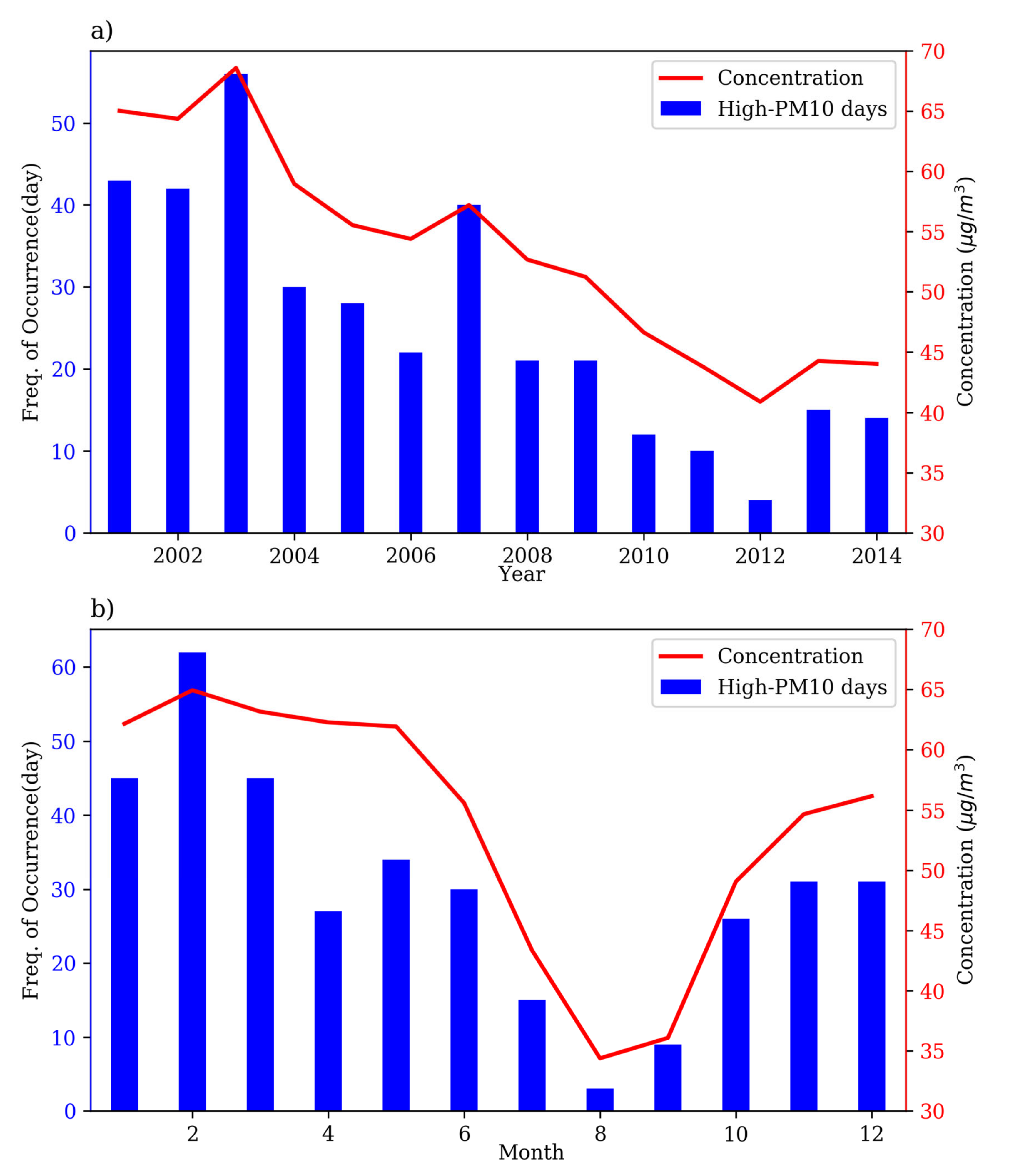
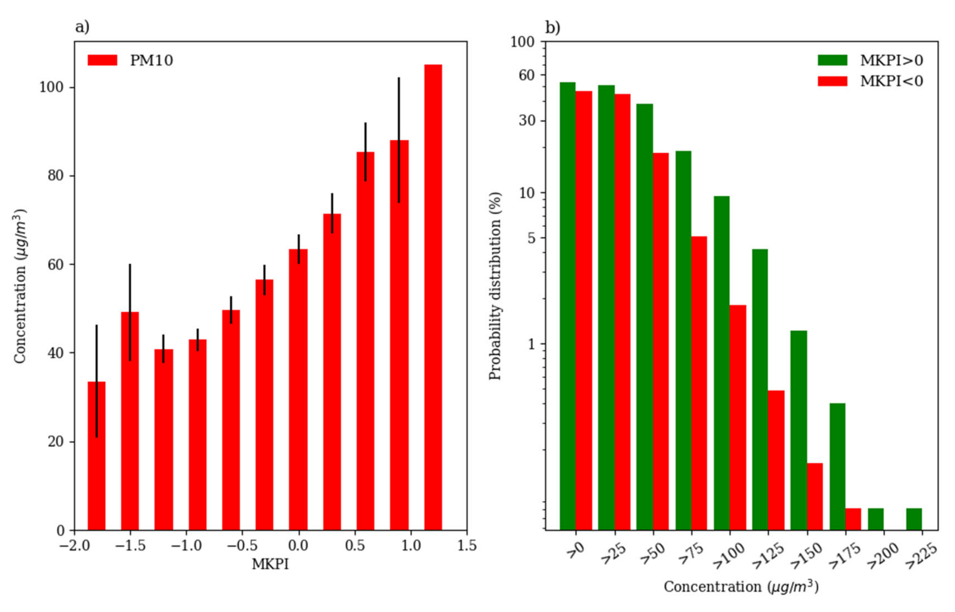
3.1. Characteristics of PM₁₀ in Seoul

PM₁₀ concentrations and high PM₁₀ episodes in Seoul were investigated using station and reanalysis data. High PM₁₀ episodes occurred on 358 days between 2001 and 2014 (25.6 d/y). The daily mean PM₁₀ concentration was 53.3 µg/m³ and the standard deviation was 29.4 µg/m³ over the entire 2001–2014 period. Owing to the implementation of the air pollution management policies in the Seoul metropolitan area [8,9,14,25], the annual mean PM₁₀ concentrations decreased in the 2000s (red line in Figure 1a). The annual mean PM₁₀ concentration in Seoul decreased below the South Korean air quality standard (yearly average of 50 µg/m³) from 2010 but is still twice the stipulated WHO standard (yearly average of 20 µg/m³). The PM₁₀ concentration in Seoul increased slightly due to the longer lifetime of the pollutants because of the weakening of the surface wind speed from 2012 [26]. The monthly mean PM₁₀ concentrations were higher in the winter than in the summer (June–July–August (JJA)) (Figure 1b). The lower PM₁₀ concentration in summer is probably because of the absence of pollution due to heating. Moreover, rainfall has a wet scavenging effect that sinks the dust from the atmosphere [26,27,28]. In South Korea, rainfall is concentrated in the summer and is associated with the East Asian Summer Monsoon (EASM). The wet scavenging effect is greater in the summer than in the winter [26].

High PM₁₀ episodes in the winter occurred on 138 days (9.8 d/y), accounting for 38.5% of the total high PM₁₀ episodes. Contrastingly, high PM₁₀ episodes in the summer occurred for a total of 48 days (3.4 d/y), which is 13.4% of the total high PM₁₀ episodes (Figure 1b). According to previous studies [8,10], the occurrence of high PM₁₀ episodes in the winter is more frequent because of a mix of local and external emissions; however, in the summer, they are due to local emissions.

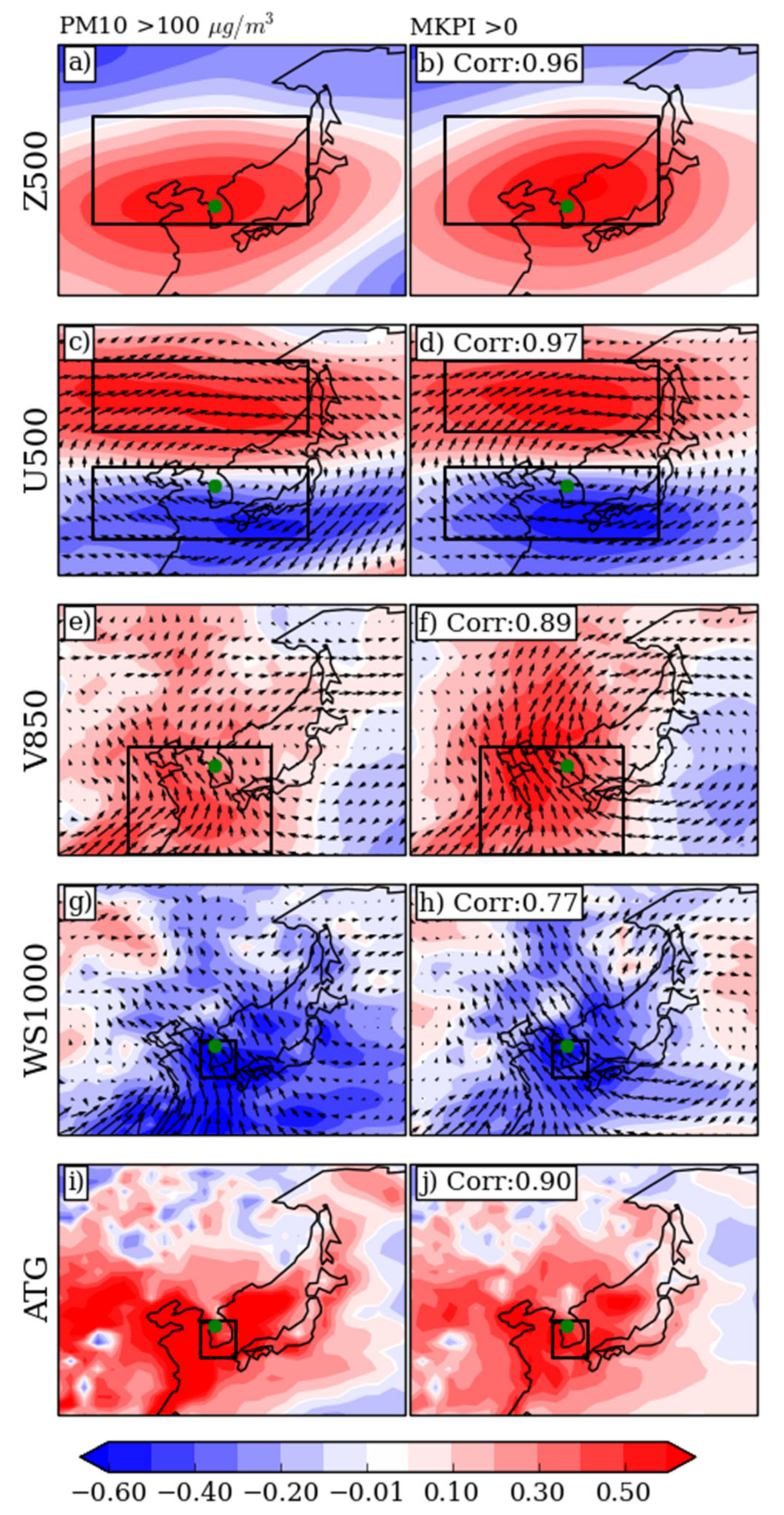
3.2. Atmospheric Patterns Related to High PM₁₀ Concentrations

Normalized anomalous atmospheric patterns of the three variables (Z500, U500, and V850) and the horizontal and vertical ventilation variables (WS1000 and ATG) were examined from the high PM₁₀ episodes (138 days) during the winter (Figure 2).

First, a positive geopotential anomaly at 500 hPa occurred over the Korean peninsula during the high PM₁₀ episodes (Figure 2a). Seoul is located to the south of the anomalous high pressure where the anomalous high pressure works to weaken zonal winds (Figure 2c). The reduction in the vertical shear of horizontal winds weakens the synoptic disturbances and vertical mixing of the atmosphere [8,10,12,14,19]. Therefore, it is a favorable environment for the accumulation of pollutants in Seoul.

Second, weak northerly surface winds over South Korea (Figure 2g) cause positive temperature anomalies in the Yellow Sea, and increased temperature can enhance chemical reactions associated with anthropogenic aerosol formation [29]. In addition, the composite vertical temperature of the 138 high PM₁₀ episodes feature warm anomalies at around 925 hPa over South Korea (35N–37° N, 125–127° E), showing a characteristic strengthening of the reverse layer between 1000 hPa and 925 hPa (not shown). The results are the same as those of the high PM₁₀ episodes in previous studies [8,18], and the enhanced thermal stability of the lower atmosphere can prevent the vertical dispersion of pollutants [10,18].

Third, PM₁₀ concentration in the East China Plain (ECP) is closely correlated with both ventilation indices (WS1000 and ATG) [17], whereas PM₁₀ in Seoul and South Korea shows high correlation only with WS1000 [14]. Because the ECP is a basin surrounded by mountainous regions, wind circulation is blocked, and temperature reversals occur frequently allowing local emission to be trapped in the lower atmosphere as South Korea is mainly affected by horizontal transport and diffusion rather than vertical diffusion because it is surrounded by sea on three sides [14].

Fourth, South Korea is located in an area of prevailing westerly winds, which are known to transport pollution from the industrial cities such as Beijing, Tianjin, and Shanghai to South Korea [8,10,11,12]. Lee et al. [10] tried to explain the transport of pollutants by the lower meridional winds (V850); however, results showed the lowest correlation with the total PM₁₀ concentration in Seoul (Table 2). V850 does not take into account the transport of pollutants in accordance with the two different patterns: from Shanghai (31.2° N) to Seoul (36.5° N) through the southwesterly winds and from Beijing (39.9° N) and Tianjin (39.1° N) to Seoul (36.5° N) through the northwesterly winds. However, the weather patterns in the high PM₁₀ episodes were caused by anomalous southwesterly winds over the Yellow Sea, which are favorable for the transport of pollutants from Shanghai to Seoul, while those from Beijing to Seoul could be reduced (Figure 2e). The correlation between V850 and horizontal ventilation (WS1000) is −0.75 at the 1% significance level. This correlation means that if the southerly wind anomalies are strengthened then the surface wind speed in South Korea will weaken and horizontal ventilation will decrease.

Depending on anomalous atmospheric fields, it is possible to estimate the origin of the pollutants transported into Seoul from the industrial facilities located across the Yellow Sea; however, it is difficult to quantify pollutants from China’s two major industrial facilities. When the anomalous southwesterly wind increases, the horizontal ventilation decreases in South Korea and the average weather pattern suitable for high PM₁₀ episodes occurs, which leads to its high concentration. In the case of northwesterly winds, the transport of pollutants from Beijing and Tianjin to South Korea will increase when compared with those during an average climate, but horizontal ventilation in South Korea will be strengthened. Thus, favorable conditions for PM₁₀ accumulation include an increase in the amount of pollutants and stagnant atmospheric conditions such as weak horizontal ventilation at the surface level and upper-level high patterns. Therefore, near-surface horizontal ventilation (WS1000) and upper zonal wind patterns (U500) are key factors that can predict PM₁₀ concentrations. These factors were adapted to develop a new index.

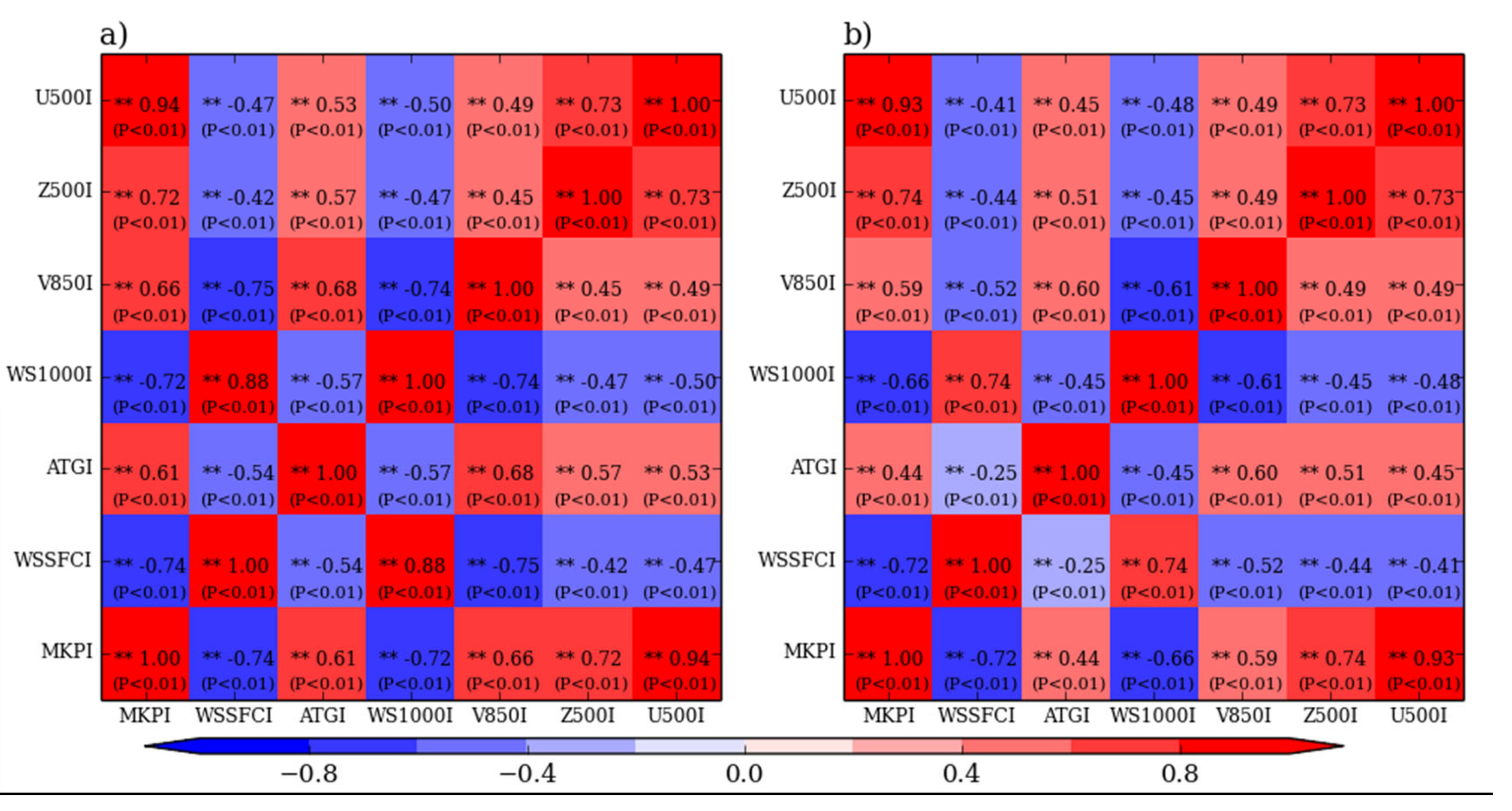
3.3. MKPI Development

Figure 3 represents the spatial correlation between the daily PM₁₀ and the five indices (Z500I, U500I, V850I, WSSFCI, and ATGI) during the winters of the 2001−2014 period. Instead of WS1000I, the 10 m wind speed index (WSSFCI) was used for the analysis (Table 2). The location U500I, as defined by [10], showed the highest correlation with PM₁₀ (black boxes in Figure 3b). On the other hand, WS1000I showed a higher correlation with daily/monthly PM₁₀ in the area (25° E–40° N, 115° E–135° E) (black boxes in Figure 3d), including China’s industrial facilities located on the Yellow Sea and those in South Korea (33–38° N, 125–130° E) defined by [14].

We also calculated NWSSFC by multiplying the negative value by WSSFC, which has a negative correlation with PM₁₀ unlike that of U500. The MKPI, which improves the KPI index of [10], was developed using U500 and NWSFC. As the positive value of the MKPI increases, the pressure in the upper atmosphere increases over the Korean peninsula and the horizontal ventilation effects decrease, implying that stagnant atmospheric condition is strengthened.

In Table 2, the MKPI is significantly correlated with daily PM₁₀ (r = 0.42) and monthly PM₁₀ (r = 0.66) values at the 1% significance level. This is an improvement compared to previous indices (Table 2). The composite weather patterns for positive MKPI are very similar to atmospheric conditions for high PM₁₀ episodes (Figure 2). The pattern correlations between the two composites were the highest with a U500 of 0.97 and WS1000 of 0.77 (Figure 2).

In addition, the MKPI is significantly correlated with other indices exceeding 0.61 at the 1% significance level, which means that it reflects the atmospheric pattern characteristics associated with the high PM₁₀ episodes (Figure 4a). Therefore, the positive value of the MKPI is effective in representing the weather conditions of high PM₁₀ episodes.

Figure 5 shows the distribution of PM₁₀ concentrations within each 0.3 bin between −1.8 and 1.5 of the MKPI and the frequency distribution of the MKPI within each 25 µg/m³ bin between 0 and 250 µg/m³ of PM₁₀ concentration. The PM₁₀ concentration within each 0.3 bin gradually increased with a positive value. In particular, the mean PM₁₀ between 0 and 0.3 was approximately 63.3 µg/m³, which is larger than the average background concentration of 53.3 µg/m³ in Seoul (Figure 5a).

In addition, the frequency of stagnant atmospheric conditions (MKPI > 0) in PM₁₀ cases increased with increasing PM₁₀ concentrations (Figure 5b), similarly as in Hong et al. [5]. Within the 14-year PM₁₀ observations, there were 138 high PM₁₀ days with PM₁₀ > 100 µg/m³, out of which 116 days had an MKPI > 0 and 55 days an MKPI > 0.5. Thus, 84% (116/138) of all the observed high PM₁₀ episodes occurred with an MKPI > 0. Over the 14-year study period, 655 days had an MKPI > 0 and 195 days had an MKPI > 0.5. That is, 17.7% (116/655) of the days had an MKPI > 0 and 28% (55/195) had an MKPI > 0.5 indicating high PM₁₀ episodes (Figure 5). Therefore, MKPI effectively reflects the atmospheric conditions associated with PM₁₀ concentrations in Seoul.

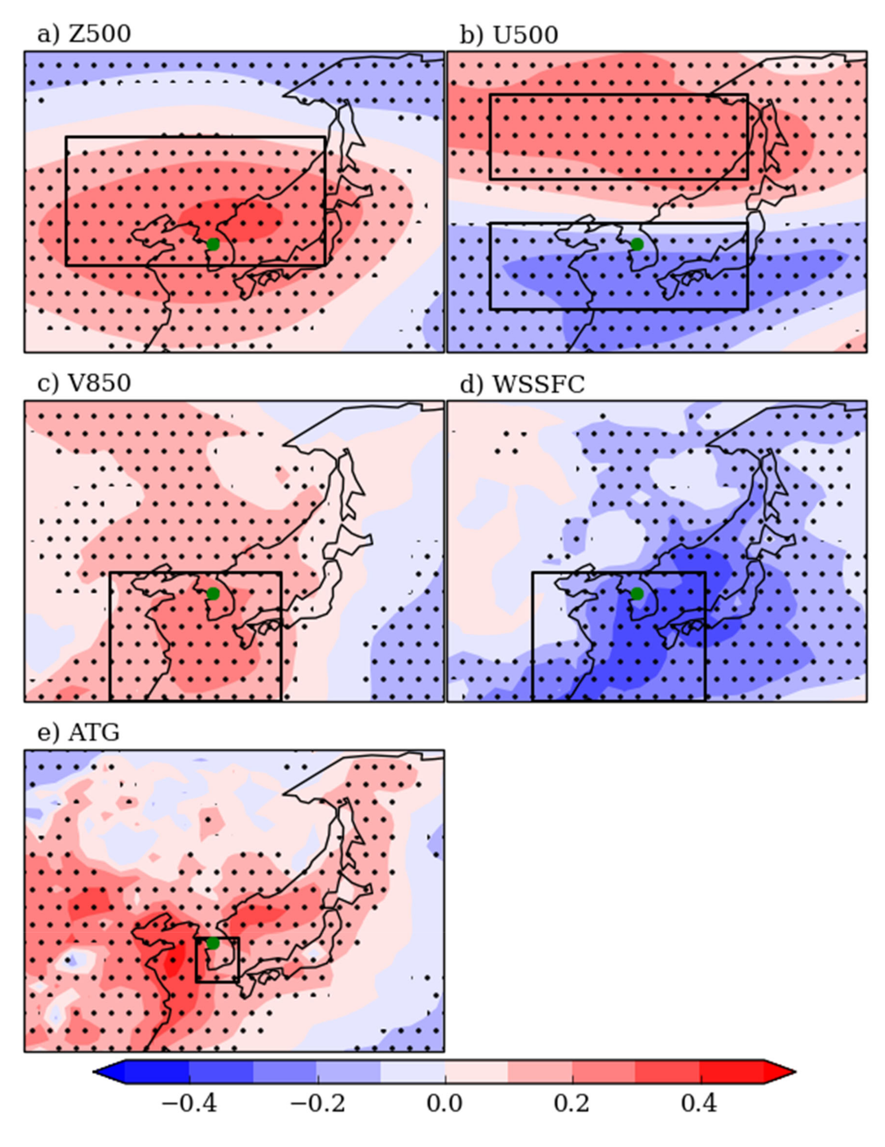
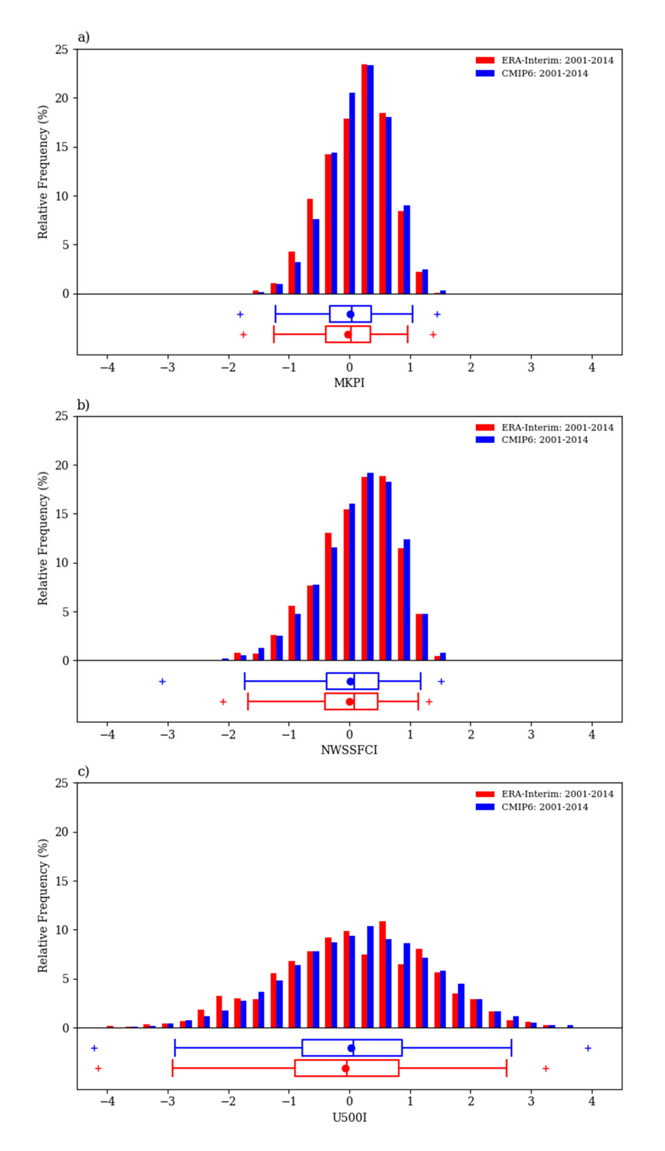
3.4. Validation of Applicability within the CMIP6 of the MKPI

The CMIP6 models used in this study are characterized by the oversimplification of the surface wind speed in the East Asian region compared to the ERA-Interim reanalysis data, while the east–west wind speed at 500 hPa is slightly underestimated (not shown). Thus, we used the reanalysis data to verify whether the improved MKPI was applicable to CMIP6.

First, CMIP6 models were analyzed for the correlation between atmospheric variables. The results showed that the correlation between the atmospheric variables in the CMIP6 ensemble was slightly lower than in the reanalysis data, but it was mostly similar and significant (Figure 4b). However, ATG, which is calculated as a vertical potential temperature difference of 925 hPa and 1000 hPa, showed a low correlation with other meteorological variables. This is because the calculation area of the ATG included the mountainous terrain of the Korean peninsula, which means that the differences in the mask between two pressure levels (925 hPa and 1000 hPa) resulted in a slightly lower correlation with other weather variables.

Figure 6 shows the histogram of the three indices (MKPI, NWSSFCI, and U500I) derived from both ERA-Interim and CMIP6 models. The distribution of the range, mean, and median of the variables calculated in the model and that in the reanalysis were consistent (Figure 6b,c). MKPI was normalized by averaging two factors: NWSSFC and U500. The distribution of the MKPI from ERA-Interim and CMIP6 shows a good agreement (Figure 6a).

Thus, the CMIP6 models simulate the atmospheric interrelationships as the correlation between the atmospheric variables is similar to that of the ERA-Interim data (Figure 4b). In addition, in spite of the uncertainty in the data of the CMIP6 model, both the CMIP6 and ERA-Interim models expressed similar frequency distributions of the MKPI similar to in the normalized method (Figure 6). The four types of SSP scenarios that were used for the future projections of weather patterns related to PM₁₀ are described in the next section.

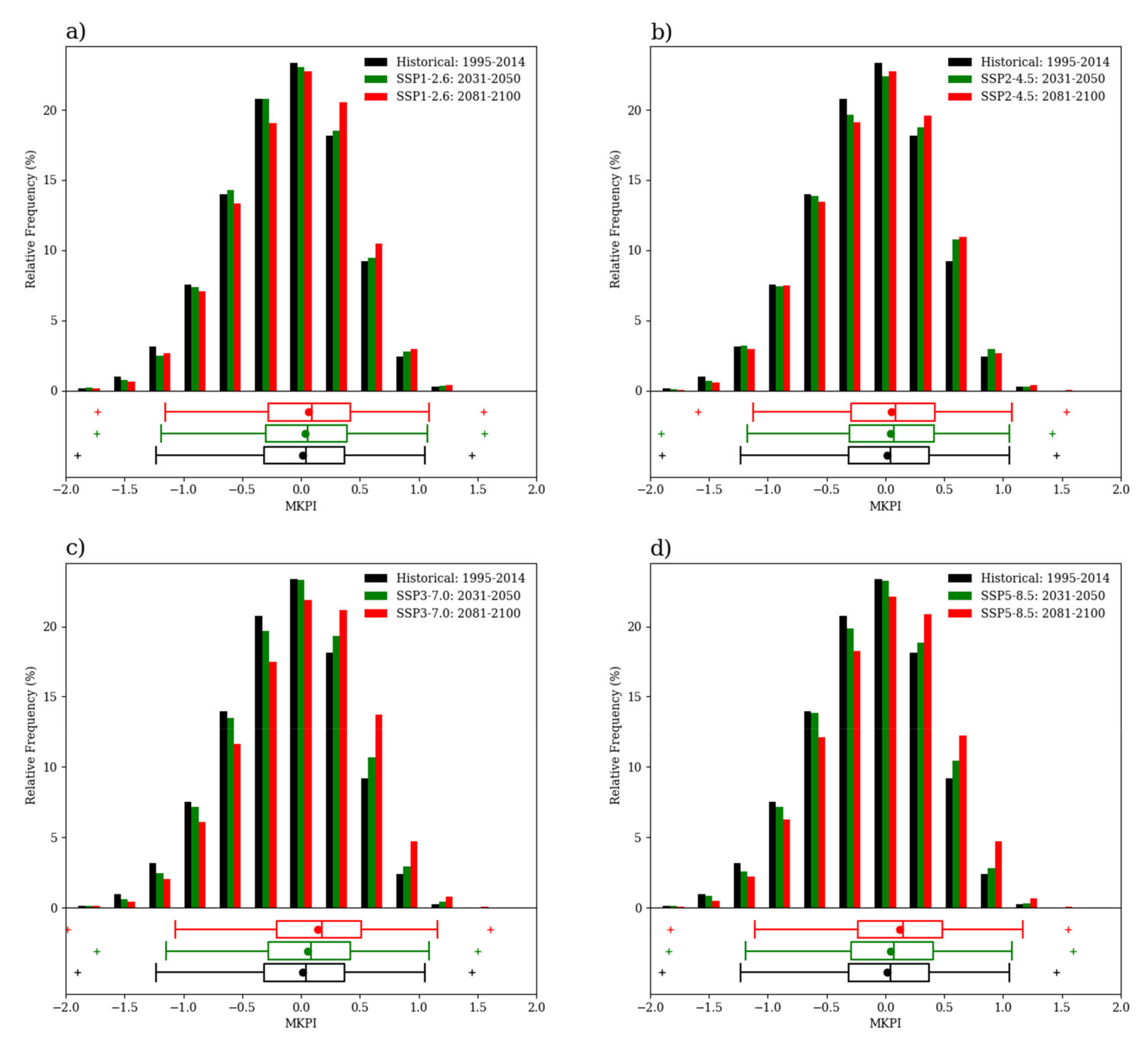
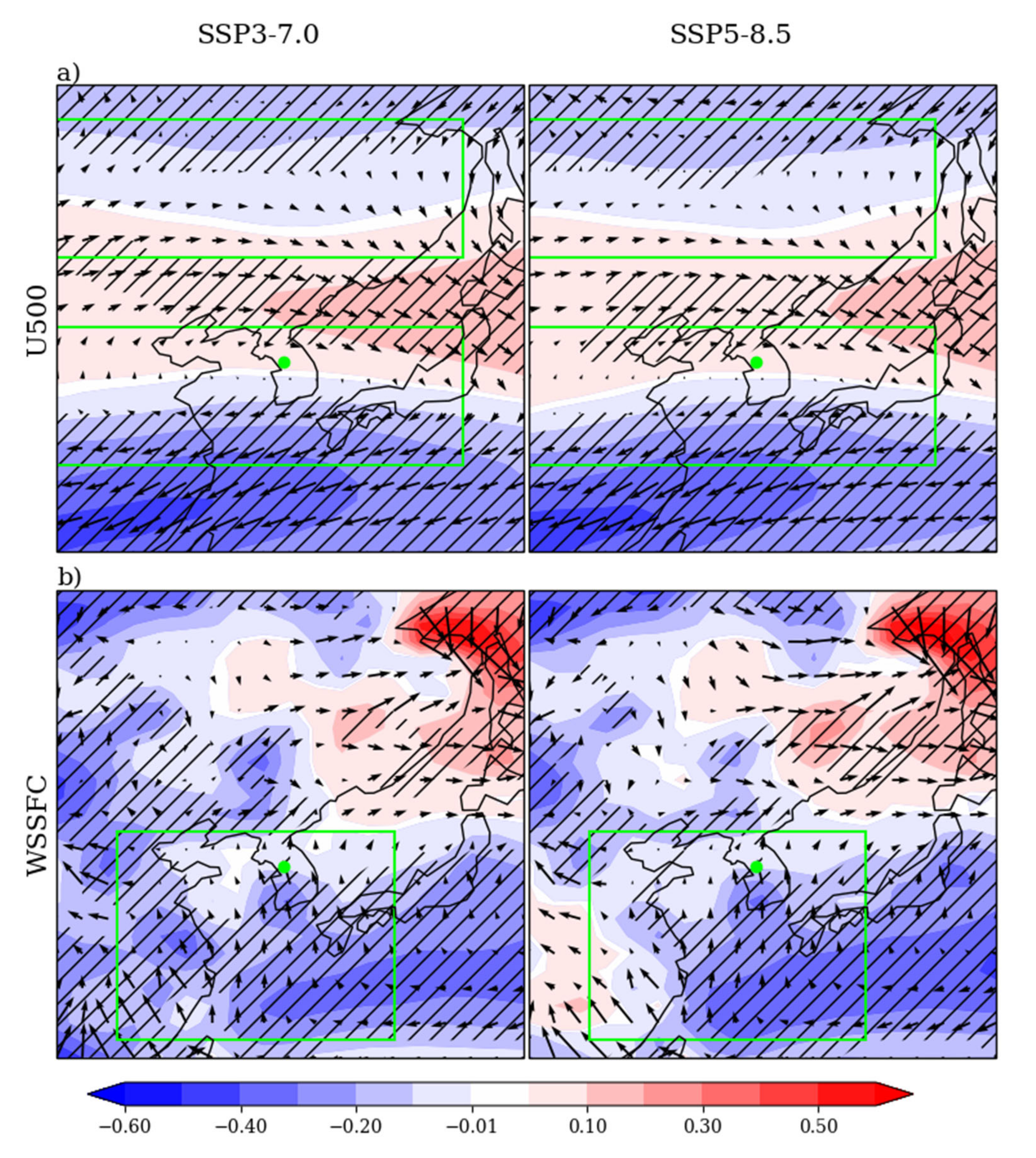
3.5. Future Projections of the MKPI

In this study, using the ensemble of CMIP6, the frequency of weather patterns related to a high PM₁₀ concentration was compared for the three periods: present (1995–2014), near-term future (2031–2050), and long-term future (2081–2100).

The MKPI for future scenarios were calculated using Equations (8)–(12). The two indices, U500I and WSSFCI, were normalized using the mean and standard deviation values of the reference period (1981–2010) on the historical simulation; then, NWSSFC was calculated by multiplying the negative value by WSSFC. After averaging, the two normalized daily anomalies were renormalized using the standard deviation of the reference period. Figure 7 represents the MKPI frequency and box plot for the three periods. The mean value of the MKPI increased in the future scenarios, and the change in the mean value was greater in the long-term future scenario than in the near-term future scenario. In other words, climate change is expected to increase the frequency of atmospheric patterns corresponding to MKPI > 0 that are favorable for high PM₁₀ concentrations.

Table 3. Change in frequency for different winter MKPI values. The columns show historical (1995–2014), near-term future (2031–2050), and long-term future (2081–2100) climates and standard deviation (in parentheses) of the frequency in the interrelationships (days per season), respectively.

Frequency of the MKPI
Period	Scenario	(>0)	(0–0.5)	(0.5–1)	(>1)
1995–2014	HIST	48.1 (±2.06)	32.7 (±2.04)	14 (±1.13)	1.3 (±0.16)
2031–2050	SSP1-2.6	48.7 (±3.15)	32.4 (±2.33)	14.8 (±0.89)	1.5 (±0.58)
	SSP2-4.5	49.6 (±2.85)	32.2 (±1.72)	16.1 (±2.11)	1.3 (±0.4)
	SSP3-7.0	50.9 (±3.29)	33.3 (±1.13)	15.9 (±2.1)	1.7 (±0.42)
	SSP5-8.5	50.1 (±1.29)	32.9 (±1.27)	15.6 (±1.25)	1.6 (±0.45)
2081–2100	SSP1-2.6	51.4 (±3.8)	33.7 (±1.97)	16.1 (±2.69)	1.6 (±0.41)
	SSP2-4.5	50.7 (±3.19)	32.9 (±1.57)	16.3 (±1.75)	1.5 (±0.42)
	SSP3-7.0	56 (±2.09)	32.9 (±1.48)	20.4 (±2.32)	2.8 (±1.02)
	SSP5-8.5	54.6 (±2.37)	32.9 (±1.14)	18.8 (±1.21)	2.8 (±0.58)

shows the frequency of the positive MKPIs for the three periods with the ensemble mean and standard deviation for the CMIP6 models. As a result of the four SSPs, the frequency of MKPI > 0 is expected to increase from 0.6 days (1.2%) to 2.8 days (5.8%) in the near-term future, and 2.6 days (5.4%) to 7.9 days (16.4%) in the long-term future. Cai et al. [18] defined weather conditions conducive to Beijing’s severe haze event during wintertime and its features were very similar to that of MKPI > 0. They projected a nine-times increase in the frequency of conducive weather conditions by the end of the 21st century compared to historical conditions. In contrast, as a result of applying the geopotential height (Z500), as defined by Lee et al. [10], to the four chosen SSPs, the frequency of Z500 > 0 is expected to increase from 20.6 days to 38.1 days in the long-term future (2081–2100) compared to the present (1995–2014). The overestimation of the results in this study is because of the increase in geopotential height with increasing air temperature due to climate change.

The increases in the frequency of anomalous weather conditions are conducive to large-scale changes. Events such as the weakening of the East Asian winter monsoon due to reductions in the temperature difference between land and ocean, faster warming in the lower troposphere, and weakening of the northwesterly wind caused by the reduction in the land–sea temperature contrasts, surface air pressure increase at the midlatitudes, and decreases in polar regions affect the weakening of the northwesterly winds in the East Asia regions [18]. All these large-scale changes are associated with global greenhouse gas emissions; however, MKPI > 0 occurred more frequently in SSP3-7.0 than in SSP5-8.5, with greater radiative forcing. Figure 8 shows the differences in the composite pattern anomalies of winter between the present and long-term future in the two scenarios of SSP3-7.0 and SSP5-8.5.

The two future scenarios commonly indicate the strengthening of weather conditions for MKPI > 0, including the enhancement of high circulation at 500 hPa on the Korean peninsula (Figure 8a) and weakening winds from the Yellow Sea (Figure 8b). In particular, the intensity of change in SSP3-7.0 was greater than in SSP5-8.5. As a result, it is assumed that the SSP scenarios would have had a more complex effect on future changes than the RCP scenarios of the CMIP5 because they take into account changes in both greenhouse gases and socioeconomics.

4. Summary

This study examined atmospheric patterns related to the PM₁₀ concentrations over the Seoul metropolitan area using data from 25 stations in Seoul for the 2001–2014 period. A new index, MKPI, was developed by analyzing various atmospheric variables related to the high PM₁₀ episodes in Seoul, South Korea, and the following features were discovered.

PM₁₀ concentration over the Korean peninsula is known to be affected by regional emissions and the transport of pollutants from China’s industrial locations across the Yellow Sea. Based on the results obtained by applying the normalized anomaly method to the analysis of high PM₁₀ episodes, anomalous weather patterns during these episodes were conditioned to increase or decrease the transportation of pollutants from Shanghai, Beijing, and Tianjin, which are located south and north of Seoul. Furthermore, high PM₁₀ episodes occurred despite weather conditions that could reduce the transportation of emissions from Beijing and Tianjin because of the weakened surface wind speed in the Korean peninsula, which caused a decrease in horizontal ventilation, creating favorable conditions for the generation of high concentrations of PM₁₀.

Among the 138 high PM₁₀ episodes, the frequency of MKPI > 0 accounted for approximately 84% (116 days) and the MKPI effectively reflected atmospheric conditions. CMIP6 has been shown to simulate the frequency distribution of the MKPI calculated through standardization methods and the correlations between atmospheric variables are very similar to those of the observed values. In other words, MKPI can be applied without model bias correction. According to the four scenarios considered (SSP1-2.6, SSP2-4.5, SSP3-7.0, and SSP5-8.5), the number of days of MKPI > 0 was expected to increase from 0.6 (1.2%) to 2.8 (5.8%) days in the near-term future (2031–2050) and 2.6 (5.4%) to 7.9 (16.4%) days in the long-term future (2081–2100) compared to the present (1995–2014). Similar results were reported in [18].

According to earlier CMIP5 results with RCPs, the frequency of the number of atmospheric patterns favorable for high PM₁₀ concentration will increase with larger radiative forcing scenarios [10,18]. However, the new SSPs considered in the CMIP6 provide different results. The SSP3-7.0 predicted that the frequency of MKPI > 0 would be more frequent than that of SSP5-8.5, even though the radiative forcing was less than that of SSP5-8.5 (Table 3). Atmospheric patterns associated with high PM₁₀ concentrations are very complex phenomena that are affected by a variety of remote correlations such as influences of Arctic sea ice, the Aleutian low pressure, and the Western Pacific high pressure [14,18,19,30,31].

In addition, SSPs include forms of socioeconomic development into the RCPs such as the changes in population, economic development, land use, and technology, which can affect radiative forcing and climate. Further studies will require a more detailed investigation of the causes for the changes in atmospheric patterns using multiple ensemble models from CMIP6. This study did not distinguish whether the main source of PM₁₀ observed in Seoul was a regional pollutant or an inflow of pollutants. Therefore, it is necessary to distinguish between local and foreign influences using methods such as cluster analysis. This analysis will also be applied to SSP scenarios, which will help with long-term domestic policy related to particulate matter reduction.

References

1. Fajersztajn, L.; Veras, M.; Barrozo, L.V.; Saldiva, P. Air pollution: A potentially modifiable risk factor for lung cancer. Nat. Rev. Cancer 2013, 13, 674–678. [Google Scholar] [CrossRef] [PubMed]
2. Yasunari, T.; Niles, D.; Taniguchi, M.; Chen, D. Asia: Proving ground for global sustainability. Curr. Opin. Environ. Sustain. 2013, 5, 288–292. [Google Scholar] [CrossRef]
3. Harrison, R.M.; Yin, J. Particulate matter in the atmosphere: Which particle properties are important for its effects on health? Sci. Total Environ. 2000, 249, 85–101. [Google Scholar] [CrossRef]
4. Chen, B.; Kan, H. Air pollution and population health: A global challenge. Environ. Health Prev. Med. 2008, 13, 94–101. [Google Scholar] [CrossRef] [Green Version]
5. Hong, C.; Zhang, Q.; Zhang, Y.; Davis, S.J.; Tong, D.; Zheng, Y.; Liu, Z.; Guan, D.; He, K.; Schellnhuber, H.J. Impacts of climate change on future air quality and human health in China. Proc. Natl. Acad. Sci. USA 2019, 116, 17193–17200. [Google Scholar] [CrossRef] [Green Version]
6. The World Health Organization. Air quality guidelines global update 2005. In Proceedings of the Report on a Working Group Meeting, Bonn, Germany, 18–20 October 2005. [Google Scholar]
7. Baek, S.-O.; Koo, Y.-S. Critical evaluation of and suggestions for a comprehensive project based on the special act on seoul metropolitan air quality improvement. J. Korean Soc. Atmos. Environ. 2008, 24, 108–121. [Google Scholar] [CrossRef]
8. Lee, S.; Ho, C.-H.; Choi, Y.-S. High-PM10 concentration episodes in Seoul, Korea: Background sources and related meteorological conditions. Atmos. Environ. 2011, 45, 7240–7247. [Google Scholar] [CrossRef]
9. Ahmed, E.; Kim, K.-H.; Shon, Z.-H.; Song, S.-K. Long-term trend of airborne particulate matter in Seoul, Korea from 2004 to 2013. Atmos. Environ. 2015, 101, 125–133. [Google Scholar] [CrossRef]
10. Lee, H.-J.; Jeong, Y.; Kim, S.; Lee, W.-S. Atmospheric circulation patterns associated with particulate matter over South Korea and their future projection. J. Clim. Chang. Res. 2018, 9, 423–433. [Google Scholar] [CrossRef]
11. Lee, S.; Ho, C.-H.; Lee, Y.G.; Choi, H.-J.; Song, C.-K. Influence of transboundary air pollutants from China on the high-PM10 episode in Seoul, Korea for the period October 16–20, 2008. Atmos. Environ. 2013, 77, 430–439. [Google Scholar] [CrossRef]
12. Oh, H.-R.; Ho, C.-H.; Kim, J.; Chen, D.; Lee, S.; Choi, Y.-S.; Chang, L.-S.; Song, C.-K. Long-range transport of air pollutants originating in China: A possible major cause of multi-day high-PM10 episodes during cold season in Seoul, Korea. Atmos. Environ. 2015, 109, 23–30. [Google Scholar] [CrossRef]
13. Smith, S.; Stribley, F.T.; Milligan, P.; Barratt, B. Factors influencing measurements of PM10 during 1995–1997 in London. Atmos. Environ. 2001, 35, 4651–4662. [Google Scholar] [CrossRef]
14. Kim, J.-H.; Kim, M.-K.; Ho, C.-H.; Park, R.J.; Kim, M.J.; Lim, J.; Kim, S.-J.; Song, C.-K. Possible link between arctic sea ice and January PM10 concentrations in South Korea. Atmosphere 2019, 10, 619. [Google Scholar] [CrossRef] [Green Version]
15. Horton, D.E.; Harshvardhan; Diffenbaugh, N.S. Response of air stagnation frequency to anthropogenically enhanced radiative forcing. Environ. Res. Lett. 2012, 7, 044034. [Google Scholar] [CrossRef] [PubMed]
16. Kim, H.; Kim, S.; Son, S.-W.; Lee, P.; Jin, C.-S.; Kim, E.; Kim, B.; Ngan, F.; Bae, C.; Song, C.-K.; et al. Synoptic perspectives on pollutant transport patterns observed by satellites over East Asia: Case studies with a conceptual model. Atmos. Chem. Phys. Discuss. 2016, 1–30. [Google Scholar] [CrossRef] [Green Version]
17. Zou, Y.; Wang, Y.; Zhang, Y.; Koo, J.H. Arctic sea ice, Eurasia snow, and extreme winter haze in China. Sci. Adv. 2017, 3, e1602751. [Google Scholar] [CrossRef] [Green Version]
18. Cai, W.; Li, K.; Liao, H.; Wang, H.; Wu, L. Weather conditions conducive to Beijing severe haze more frequent under climate change. Nat. Clim. Chang. 2017, 7, 257–262. [Google Scholar] [CrossRef]
19. Oh, H.-R.; Ho, C.-H.; Park, D.-S.R.; Kim, J.; Song, C.-K.; Hur, S.-K. Possible relationship of weakened aleutian low with air quality improvement in Seoul, South Korea. J. Appl. Meteorol. Climatol. 2018, 57, 2363–2373. [Google Scholar] [CrossRef]
20. Koo, Y.-S.; Yun, H.-Y.; Kwon, H.-Y.; Yu, S.-H. A development of PM10 forecasting system. J. Korean Soc. Atmos. Environ. 2010, 26, 666–682. [Google Scholar] [CrossRef] [Green Version]
21. Kuhlbrodt, T.; Jones, C.G.; Sellar, A.; Storkey, D.; Blockley, E.; Stringer, M.; Hill, R.; Graham, T.; Ridley, J.; Blaker, A.; et al. The low-resolution version of HadGEM3 GC3.1: Development and evaluation for global climate. J. Adv. Model. Earth Syst. 2018, 10, 2865–2888. [Google Scholar] [CrossRef] [Green Version]
22. Williams, K.D.; Copsey, D.; Blockley, E.W.; Bodas-Salcedo, A.; Calvert, D.; Comer, R.; Davis, P.; Graham, T.; Hewitt, H.T.; Hill, R.; et al. The met office global coupled model 3.0 and 3.1 (GC3.0 and GC3.1) configurations. J. Adv. Model. Earth Syst. 2018, 10, 357–380. [Google Scholar] [CrossRef]
23. Lee, J.; Kim, J.; Sun, M.-A.; Kim, B.-H.; Moon, H.; Sung, H.M.; Kim, J.; Byun, Y.-H. Evaluation of the Korea meteorological administration advanced community earth-system model (K-ACE). Asia Pac. J. Atmos. Sci. 2020, 56, 381–395. [Google Scholar] [CrossRef] [Green Version]
24. Sellar, A.A.; Jones, C.G.; Mulcahy, J.P.; Tang, Y.; Yool, A.; Wiltshire, A.; O’Connor, F.M.; Stringer, M.; Hill, R.; Palmieri, J.; et al. UKESM1: Description and evaluation of the U.K. earth system model. J. Adv. Model. Earth Syst. 2019, 11, 4513–4558. [Google Scholar] [CrossRef] [Green Version]
25. Kim, H.; Kim, S.; Kim, B.; Jin, C.-S.; Hong, S.; Park, R.; Son, S.-W.; Bae, C.; Bae, M.; Song, C.-K.; et al. Recent increase of surface particulate matter concentrations in the Seoul Metropolitan Area, Korea. Sci. Rep. 2017, 7. [Google Scholar] [CrossRef] [Green Version]
26. Kim, S.; Hong, K.-H.; Jun, H.; Park, Y.-J.; Park, M.; Sunwoo, Y. Effect of precipitation on air pollutant concentration in Seoul, Korea. Asian J. Atmos. Environ. 2014, 8, 202–211. [Google Scholar] [CrossRef] [Green Version]
27. Loosmore, G.A.; Cederwall, R.T. Precipitation scavenging of atmospheric aerosols for emergency response applications: Testing an updated model with new real-time data. Atmos. Environ. 2004, 38, 993–1003. [Google Scholar] [CrossRef]
28. Choi, Y.-S.; Ho, C.-H.; Kim, J.; Gong, D.-Y.; Park, R.J. The impact of aerosols on the summer rainfall frequency in China. J. Appl. Meteorol. Climatol. 2008, 47, 1802–1813. [Google Scholar] [CrossRef] [Green Version]
29. Van der Wal, J.T.; Janssen, L.H.J.M. Analysis of spatial and temporal variations of PM 10 concentrations in the Netherlands using Kalman filtering. Atmos. Environ. 2000, 34, 3675–3687. [Google Scholar] [CrossRef]
30. Mori, M.; Watanabe, M.; Shiogama, H.; Inoue, J.; Kimoto, M. Robust arctic sea-ice influence on the frequent Eurasian cold winters in past decades. Nat. Geosci. 2014, 7, 869–873. [Google Scholar] [CrossRef]
31. Mori, M.; Kosaka, Y.; Watanabe, M.; Nakamura, H.; Kimoto, M. A reconciled estimate of the influence of arctic sea-ice loss on recent Eurasian cooling. Nat. Clim. Chang. 2019, 9, 123–129. [Google Scholar] [CrossRef]
Figure 1. PM10 variations in Seoul during the 2001–2014 period. Annual high-concentration days and mean concentration (μg/m3) (a); monthly high-concentration days and mean concentration (μg/m3) (b). High PM10 days are defined as PM10 > 100 μg/m3 over 24 h. Yellow dust cases were excluded.
Atmosphere 11 01161 g001
Figure 2. Composite maps for high PM10 episodes (left column) and modified Korea particulate matter index (MKPI) > 0 (right column) of the anomalous 500 hPa geopotential height (shaded) (a,b), anomalous 500 hPa u-component wind (shaded) and wind (vector) (c,d), 850 hPa v-component wind (shaded) and wind (vector) (e,f), 1000 hPa wind speed (shaded) and wind (vector) (g,h), and ATG (vertical potential air temperature gradient, shaded) (i,j) during the winters of the 2001−2014 period. The green dots denote the location of Seoul (37.5° N, 127° E); black boxes denote the regions for the calculation of 5 indices (Z500, U500, V850, WS1000, and ATG), respectively. The anomalies are by reference to the daily standard deviation.
Atmosphere 11 01161 g002
Figure 3. Spatial correlations of PM10 in Seoul (37.5N, 127E) with a (a) geopotential height at 500 hPa, (b) u-wind component at 500 hPa, (c) v-wind component at 850 hPa, (d) 10 m surface wind speed, and (e) potential air temperature gradient, respectively. Green dots denote the location of Seoul; black boxes denote the regions for the calculation of 5 indices (Z500, U500, V850, WSSFC, and ATG) during the winters of the 2001−2014 period, respectively. The black dotted areas indicate significant regions at the 95% confidence level based on the Student’s t-test.
Atmosphere 11 01161 g003
Figure 4. Correlation matrix between the individual indices (MKPI, WSSFCI, ATGI, WS1000I, V850I, Z500I, and U500I) on ERA-Interim (a) and CMIP6 (b) during the winters of the 2001–2014 period. ** indicates statistical significance at the 99% confidence level.
Atmosphere 11 01161 g004
Figure 5. Distribution of percentages of PM10 concentration in the winter for a given MKPI threshold value range (a), and MKPI > 0 and MKPI < 0 for a given PM10 concentration threshold value range (b) for the 2001–2014 period. Error bars indicate significance at the 95% confidence intervals.
Atmosphere 11 01161 g005
Figure 6. Histogram showing the frequencies of occurrence (in percent) of daily indices: (a) modified Korea particulate index (MKPI), (b) negative wind speed at surface index (NWSSFCI), (c) 500 hPa u-wind index (U500I) for ERA-Interim and CMIP6 ensemble models during the winters of the 2001–2014 period. The horizontal boxplots show the solid horizontal lines within each ‘box’ representing the median, and the circle markers indicate the mean. The interquartile range is 25th and 75th percentiles. The ‘whiskers’ represent the 1st and 95th percentile. The cross-markers denote the highest or lowest ‘outlier’ of each case. Results for ERA-interim (red) and CMIP6 (blue) are shown.
Atmosphere 11 01161 g006
Figure 7. Similar to Figure 6 but projected for the near-term future (green bars and boxplots, 2031–2050) and long-term future (red bars and boxplots, 2081–2100) of the MKPI on the shared socioeconomic pathway (SSP) scenarios of SSP1-2.6 (a), SSP2-4.5 (b), SSP3-7.0 (c), and SSP5-8.5 (d) with the historical present (black bars and boxplots, 1995–2014).
Atmosphere 11 01161 g007
Figure 8. Differences in the composite pattern anomalies of winter between the long-term future (2081–2100) and historical period (1995–2014) of MKPI > 0 conditions near Seoul (37.5N, 127E). (a,b) Differences in flow at 500 hPa and surface (long-term future minus historical) for SSP3-7.0 (left) and SSP5-8.5 (right). The green dots denote the location of Seoul; green boxes denote the regions for the calculation of U500 and WSSFC. The stippling areas indicate significant regions at the 95% confidence level based on the Student’s t-test.
Atmosphere 11 01161 g008