North–South Discrepancy of Interannual Sea Surface Temperature Anomalies over the South China Sea Associated with Eastern Pacific El Niño Events in the Spring

Abstract

This paper discovers a spatial feature of interannual sea surface temperature (SST) anomalies over the South China Sea (SCS) in the boreal spring, based on the Simple Ocean Data Assimilation (SODA) monthly data in the period from January 1958 to December 2010. The Empirical Orthogonal Function (EOF) analysis of interannual SST anomalies shows a north–south discrepant pattern of the first mode, which is characterized by higher (lower) anomalies in the northern (southern) SCS and possessing seasonal phase locking (in the boreal spring). Besides, the high correlation coefficient between the time series of the first EOF mode and the Nino 3 SST anomalies during winter reveals that this discrepant pattern is likely caused by El Niño events. The composites of SST anomalies show that this discrepant pattern appears in the eastern Pacific (EP) El Niño events, while it does not exist in the Central Pacific (CP) El Niño events. It is believed that the western North Pacific anticyclone (WNPA) plays a key role in conveying the El Niño impact on the interannual variabilities of SCS SST in the EP El Niño events. The anomalous anticyclone in the Philippine Sea weakens the northeasterly monsoon over the SCS by its southwest portion during the mature phases of the EP El Niño events. This anomalous atmospheric circulation contributes to the north–south discrepant pattern of the wind stress anomalies over the SCS in the EP El Niño mature winters, and then leads to the north–south dipole pattern of the contemporaneous latent heat flux anomalies. The latent heat flux is a major contributor to the surface net heat flux, and heat budget analysis shows that the net heat flux is the major contributor to the SCS SST anomalies during the spring for the EP El Niño events, and the north–south discrepancy of SCS SST anomalies in the succeeding spring is ultimately formed.

1. Introduction

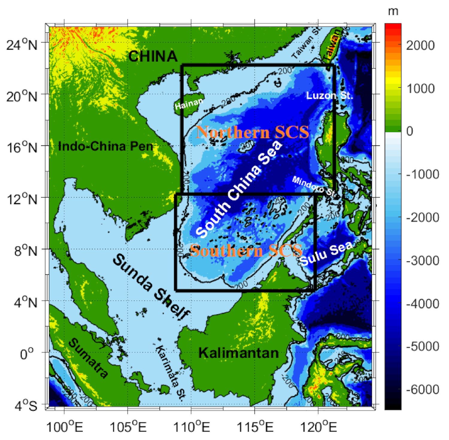
The South China Sea (SCS) is one of the largest marginal seas of the western Pacific Ocean. It is a semi-closed deep basin and embraced by the Asian continent, the Indo-China Peninsula, the Kalimantan, the Philippines and the Taiwan Island. It connects with the Pacific, East China Sea, and Sulu Sea through the Luzon Strait, Taiwan Strait, and Mindoro Strait, respectively (Figure 1). During the boreal winter, the SCS is dominated by the northeasterly monsoon, while by the southwesterly monsoon during the boreal summer. The winter monsoon is much stronger than the summer monsoon, and the annual mean wind is roughly northeasterly wind [1,2,3]. It is widely recognized that the climate of the SCS has a strong relationship with El Niño–Southern Oscillation (ENSO) [4,5,6,7,8,9,10].

Previous studies have researched the relationship between SCS sea surface temperature (SST) and ENSO. Tomita and Yasunari [6] earlier pointed out that anomalous SST over the SCS is closely related to ENSO. Klein et al. [11] revealed that positive SST anomalies tended to appear in the SCS during the mature winter and the later seasons of El Niño events. The correlation analysis revealed that the SCS SST anomalies in summer are statistically correlated with the Nino 4 Index [7] and Nino 3 Index (defined as SST anomalies averaged in 5° S–5° N, 90° W–150° W) [12]. Similarly, the time series of SCS SST anomalies lagged Nino 3 Index by 5 months [13] and lagged the Southern Oscillation Index by 7 months [14]. It is believed that ENSO exerts impact on the SCS SST via the atmospheric bridge of atmospheric circulations [11,15,16]. It is also found that the SCS SST anomalies can be modulated by the ENSO-induced ocean dynamical processes. For example, Qu et al. and Liu et al. revealed that an El Niño signal can be conveyed into the SCS through Luzon Strait [14] and Mindoro Strait, respectively [17]. In addition, Wang et al. [13] mainly told the story of the evolution of the interannual SST variability over SCS during El Niño events, and found that SCS SST interannual anomalies had “a double-peak” in the El Niño decaying years and the first and second peaks occur in February and August, respectively. The first peak is mostly caused by El Niño-induced anomalous latent heat flux and shortwave radiation, and the second peak is mainly due to the mean meridional geostrophic heat advection in the SST equation. Liu et al. [18] focused on comparing the SCS thermal variations associated with the eastern Pacific (EP) El Niño and those associated with the Central Pacific (CP) El Niño events, mainly involving “double peak” characteristics and SST evolution. They notice the west–east spatial differences of SST anomalies during CP El Niño events. Tan et al. [19] mainly revealed that the SCS SST warming occurred in the developing autumn of canonical El Niño and El Niño Modoki I, while the SST cooling appeared in the developing autumn of El Niño Modoki II. The SST cooling resulted from the west propagation of western North Pacific anticyclone (WNPA) during El Niño Modoki II.

Previous research mainly focused on the basin-wide responses of SCS SST anomalies to ENSO. Actually, the spatial differences of SCS SST interannual variabilities and their relationship with El Niño events have been noticed before. Chu et al. [20] found that the larger interannual variabilities of SST appeared in the northern SCS during October and November 1987 as well as January and February 1988. Fang et al. [21] indicated that the northern deep basin had the highest interannual SST anomalies in the SCS and supposed that the feature has connection with the anomalous local wind stress associated with El Niño. In addition, Wang et al. [13] and Tan et al. [19] also refer to the spatial differences of SCS SST anomalies associated with El Niño events. However, the clear concept as well as understanding of SCS SST north–south discrepancy and its mechanism are still incomplete. The purpose of this study is to investigate the north–south discrepancy of interannual SCS SST anomalies associated with two distinct types of El Niño events, and find the corresponding physical mechanisms of this north–south discrepancy. The results are expected to improve the understanding of the interannual variation of the SCS SST as well as arouse attention to the spatial differences of the SCS response induced by ENSO.

In recent years, a new type of El Niño called CP El Niño (also named as El Niño Modoki [22], warm pool El Niño [23], or dateline El Niño [24]) is noted. The two different types of El Niño (EP El Niño and the CP El Niño) are different in structure, evolution, and impacts on global climate [25,26,27]. The EP Niño (also named canonical El Niño [25]) is characterized by warm SST anomalies centered in the eastern equatorial Pacific attached to the coast of South America [25,26]. In contrast, the CP El Niño is characterized by its maximum anomalous SST over the central equatorial Pacific [26]. Research revealed that SCS SST anomalies induced by two types of El Niño events are different in intensities, spatial distribution as well as time evolution [18,19,28]. Therefore, we study the spatial discrepancy of SCS SST anomalies in EP and CP El Niño, respectively.

The remainder of this article is organized in the following manner. Section 2 describes the data and method in this study. In Section 3, the interannual variations of the SCS SST in spring and their spatial discrepant performances are analyzed by performing an empirical orthogonal function (EOF) analysis to SST anomalies and the results of composite analysis of SCS SST anomalies during EP El Niño and the CP El Niño events are shown. Next, we give a heat budget analysis in Section 4. Then we research the net (latent) heat flux anomalies and wind stress anomalies over the SCS in EP and CP El Niño mature winters, respectively, and provide a possible mechanism of the spatial discrepancy mentioned above. The conclusions are given in Section 5.

2. Data and Method Description

The SST and surface wind stress data are obtained from the Simple Ocean Data Assimilation (SODA) [29,30,31], version 2.2.4, which has a resolution of 0.5° (latitude) × 0.5° (longitude) and 40 vertical levels ranging from 5 to 5375 m and covers the period from January 1871 to December 2010. The results are verified by the SST data from Met Office Hadley Centre Sea Ice and Sea Surface Temperature (HadISST) dataset on a 1° × 1° grid [32]. Monthly sensible heat net flux, latent heat net flux, net longwave radiation and net shortwave radiation were obtained from NCEP Reanalysis data [33] provided by the NOAA/OAR/ESRL PSL, Boulder, Colorado, USA [34] with T62 Gaussian grid. For convenience, all data are interpolated into 1° × 1° spatial resolution and are for the period 1958–2010 in the chosen region (3.75° N~25.25° N, 104.75° E~122.25° E) covering the whole SCS.

According to Liu et al. [18], El Niño events chosen in the following analyses during the study period are identified as the EP El Niño (1965/66, 1972/73, 1982/83, 1987/88 and 1997/98) and the CP El Niño (1977/78, 1979/80, 1990/91, 1992/93, 1994/95, 2002/03, 2004/05 and 2009/10).

In order to make a comparison of the spatial differences, we divide the SCS into northern and southern parts, and the boundary is around 14° N [20,35]. For the convenience of calculating regional mean, the ranges of two parts are in the following: the northern part covers the area of 109.25° E to 120.75° E and 14.25° N to 22.25° N, while the southern part varies from 108.25° E to 118.25° E in longitude, and from 6.25° N to 14.25° N in latitude (Figure 1).

3. North–South Discrepancy of Interannual SCS SST Anomalies

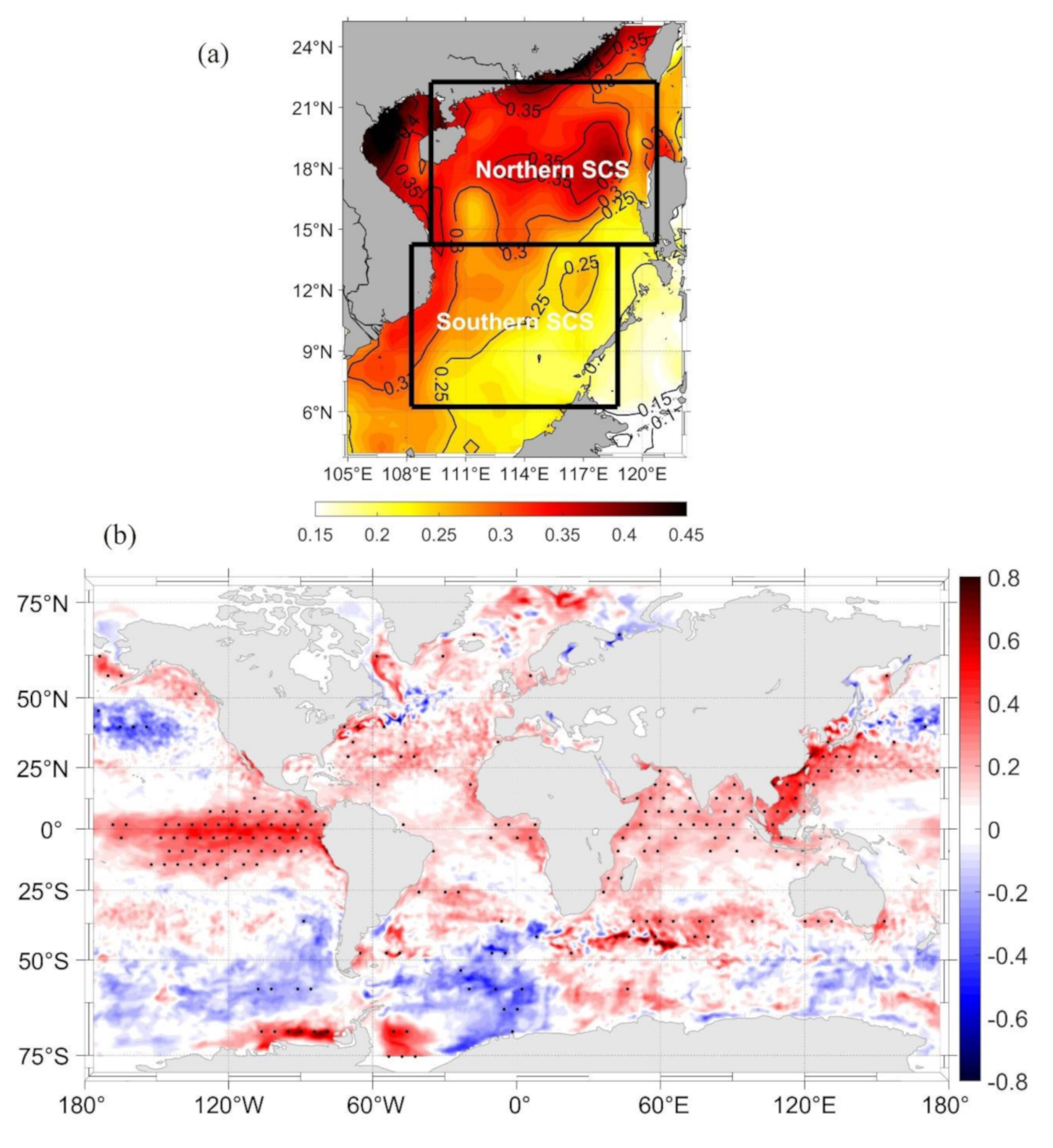
An EOF analysis is performed to research the spatiotemporal characteristics of interannual SST anomalies over SCS. The boreal spring is the chosen season to perform an EOF analysis in the below, because the mature phases of ENSO are normally in the boreal winter while its impact on other ocean basins normally peaks one or two seasons later [8]. Figure 2a presents the first EOF pattern of interannual SST anomalies in the boreal spring, which accounts for 63% of the total variances. As shown in the spatial patterns, the whole SCS is characterized with the same sign, which indicates that warming (cooling) occurs synchronously over the whole SCS. The EOF pattern in spring (Figure 2a) is characterized by a north–south discrepant pattern in the northwest–southeast direction, and the northern SCS shows evidently higher amplitude of interannual SSTA than the southern SCS. In terms of specific characteristics of spatial distribution, there is a high SST anomalies core located to the west of the Luzon Strait (around 118° E, 18° N) in the northern SCS, while in the southern SCS, higher SST anomalies appear in the western boundary of the SCS, and lower SST anomalies show in the north of Kalimantan Island. We researched the spatiotemporal characteristics of interannual SCS SST anomalies in four seasons (not shown in this paper) and found that the north–south discrepancy typically occurs in the boreal spring. In order to study the spatial discrepancy, only the SST anomalies in the boreal spring will be focused on in the following study. The correlation coefficient between the time series of the first EOF mode for spring SST anomalies over the SCS and the winter mean SST anomalies in the Nino 3 region (called Nino 3 Index below for convenience) is 0.43, which is significant at the 95% confidence level. Actually, the time series (PC1) mostly reach the peak following the positive phases of Nino 3 Index (not shown in the paper), which indicates that the SST in the SCS is modulated by El Niño events. Regressing global SST onto PC1 of SCS SST anomalies is shown in Figure 2b, we can see significant positive SST anomalies cover the entire tropical eastern Pacific with a peak near the equator, confirming a close correspondence between the leading EOF mode and SST anomalies over the tropical eastern Pacific on the interannual time scale.

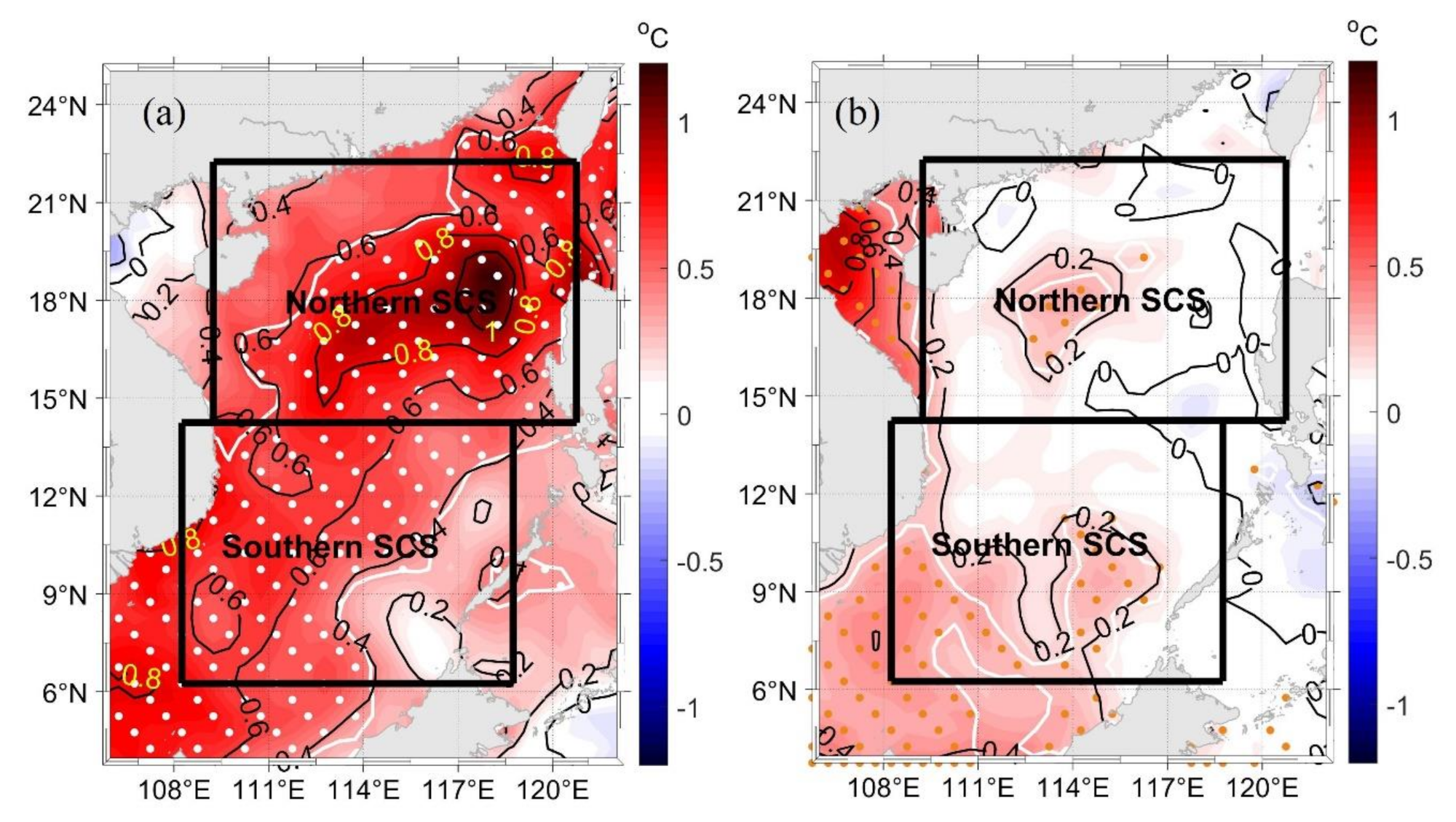
As mentioned above, there are two distinct types of El Niño (EP El Niño and the CP El Niño), whose impacts on SCS SST are different [18]. Figure 3 demonstrates the composites of SCS SST anomalies in the spring for the EP El Niño and CP El Niño in the decaying years.

For EP El Niño, the pattern of the composite of SST anomalies in the boreal spring of El Niño decaying years is very similar to the first EOF pattern in boreal spring. According to Figure 3a, the whole SCS deep basin exhibits positive SST anomalies during the spring of El Niño decaying year. The warm SST anomalies core of the northern SCS is also located in 118° E, 18° N (similar location to the high SST anomalies core of the first EOF mode), with the maximum of SST anomalies above 1.0 °C. As for the southern SCS, the warming is generally much lower than that over the northern SCS, and the warm SST anomalies decrease roughly from northwest to southeast over the southern SCS. However, for CP El Niño, although the whole SCS is also covered by positive SST anomalies, the SST anomalies are much lower than that in the EP El Niño, and there is no evident north–south discrepant pattern over SCS. The first mode of EOF shows the response of SCS SST to the EP El Niño to a certain extent, indicating the importance of the EP El Niño to the SCS SST. 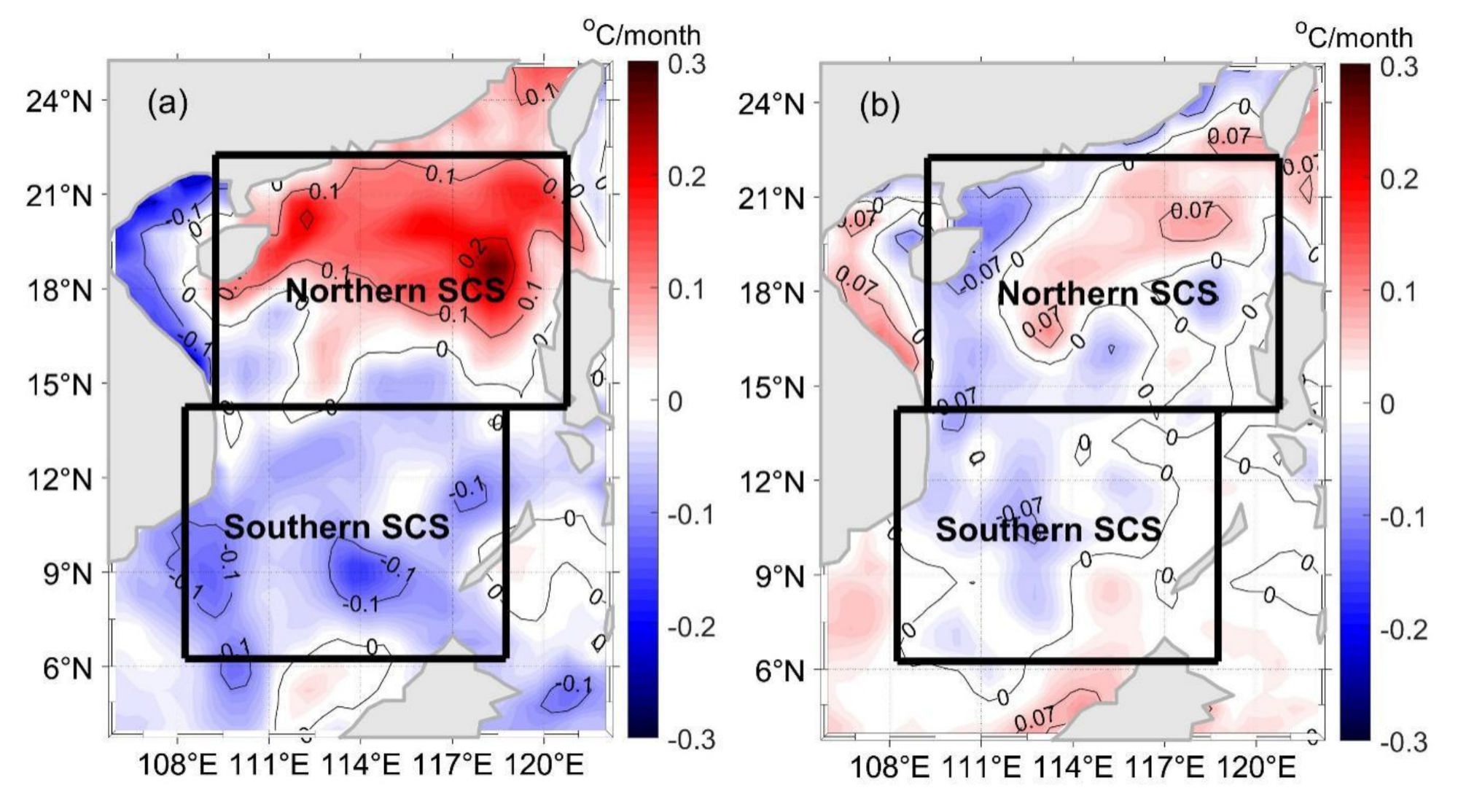The north–south discrepancy of the composite of SST anomalies in spring (Figure 3a) confirms the results revealed in Figure 2b, indicating that interannual SST anomalies over SCS has a spatial discrepant response to El Niño events, which typically appeared in EP El Niño events and also has a seasonal phase locking (in the boreal spring). The composites of the SCS SST anomalies tendencies from developing winter (December, January and February) to decaying spring (March and April) of two types of El Niño events are shown in Figure 4. For EP El Niño (Figure 4a), a dipole pattern is seen in the SCS. The warm center is still located in 118° E, 18° N (the same location mentioned in Figure 2b and Figure 3a) and the maximum of SST anomalies is close to 0.3 °C/month. However, the southern SCS is covered by cool tendency. The cool center is located around 114° E, 9° N, with minimum value lower than −0.1 °C/month. For the CP El Niño events (Figure 4b), the values of SST anomalies tendencies are much lower than that in the EP El Niño events. The obvious dipole pattern in EP El Niño (Figure 4a) does not exist in the CP El Niño events. The majority of the SCS deep basin is dominated by negative SST anomalies tendency, and positive SST anomalies tendency appears in the northeast of the SCS (the center is around 118° E, 20° N), north of the Luzon Strait, Sunda Shelf and the southeast of the SCS, respectively. The same calculation used HadISST datasets also show similar results (not shown).

4. Discussion

a.

Heat budget analysis of the SCS SST anomalies.

The atmosphere–ocean system over the SCS basin is strongly modulated by ENSO events on interannual time scales [13,19,36,37,38,39]. Wang et al. [13] pointed out a double-peak evolution of the SCS SST anomalies forced by El Niño events. The first peak in El Niño mature winters results from the altered atmospheric circulation, which contributes considerably to increasing the downward net heat flux and in turn enhances the SST warming over SCS. A mixed layer heat budget analysis is performed by using the SST equation from Qiu [40] to research the contributions of atmospheric and oceanic processes to the SCS SST anomalies for EP and CP El Niño events, and the linearized SST equation can be written as in Liu et al. [18]:

$$\begin{array}{c}\frac{\partial {T^{\prime }}_m}{\partial t}=\frac{{Q^{\prime }}_{net}}{\rho C_p{h}_m}-\left({\overrightarrow{\overline{u}}}_g·\overrightarrow{\nabla }{T^{\prime }}_m+{{\overrightarrow{u}}^{\prime }}_g·\overrightarrow{\nabla }{\overline{T}}_m\right)-\left({\overrightarrow{\overline{u}}}_e·\overrightarrow{\nabla }{T^{\prime }}_m+{{\overrightarrow{u}}^{\prime }}_e·\overrightarrow{\nabla }{\overline{T}}_m\right)\\ -\left[{\overline{w}}_e\frac{{\left(T_m-T_d\right)}^{\prime }}{h_m}+{w^{\prime }}_e\frac{\overline{\left(T_m-T_d\right)}}{h_m}\right]\end{array}$$

(1)

where T_m is the mixed-layer temperature. Q_net is the net surface heat flux, ρ = 1024 kg·m⁻³ is the density of seawater, C_p = 4007 J·kg⁻¹·K⁻¹ is the specific heat of seawater, h_m is mixed layer depth, ${\overrightarrow{u}}_e$ is the Ekman velocity, w_e is vertical entrainment rate, T_d is the water temperature below the base of the mixed layer, and ${\overrightarrow{u}}_g$ is the surface geostrophic velocity. The terms of Equation (1) represent the tendency of SST anomalies, net heat flux anomaly forcing, mean Ekman heat advection, anomalous Ekman heat advection, mean geostrophic heat advection, anomalous geostrophic heat advection, mean entrainment heat advection and anomalous entrainment heat advection, respectively. According to Liu et al. [18], the amplitude of the anomalous vertical entrainment heat flux is smaller than that of the other terms in the SST equation, and therefore the last two terms will not be discussed in this paper.

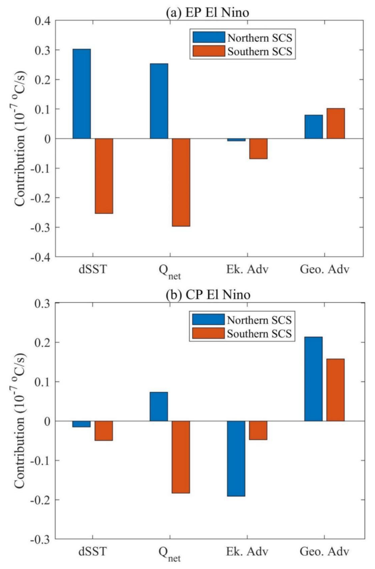
As seen from Figure 5a, for EP El Niño events, the tendency of SST anomalies in the northern SCS is positive, while it is negative in the southern SCS. From the heat budget averaged over the SCS, the net surface heat flux is the dominant contributor to the warming (cooling) tendency over the northern (southern) SCS, while Ekman heat advection and geostrophic heat advection have little influence. However, for the CP El Niño events (Figure 5b), the tendency of SST anomalies is much smaller than that in EP El Niño events. Among them, the northern SCS is mainly affected by Ekman heat advection and geostrophic heat advection, while the southern SCS is mainly influenced by net surface heat flux anomalies and geostrophic heat advection. This suggests that the response of SCS SST anomalies to CP El Niño has a different mechanism between northern and southern SCS. The mechanism of impacting SCS SST anomalies is also more complex in CP El Niño events.

According to the previous research [13,19], the net heat flux anomalies include the components of latent heat flux anomalies, sensible heat flux anomalies, shortwave radiation anomalies and longwave radiation anomalies. Among them, the anomalous latent heat flux and shortwave radiation are considered to be major contributors to the positive net heat flux anomalies during the first peak of SCS SST anomalies, and the anomalous latent heat flux is the more principal one. The sensible heat flux and longwave radiation anomalies are negligible, since their amplitudes in the SCS are smaller than that of the shortwave radiation and latent heat flux anomalies.

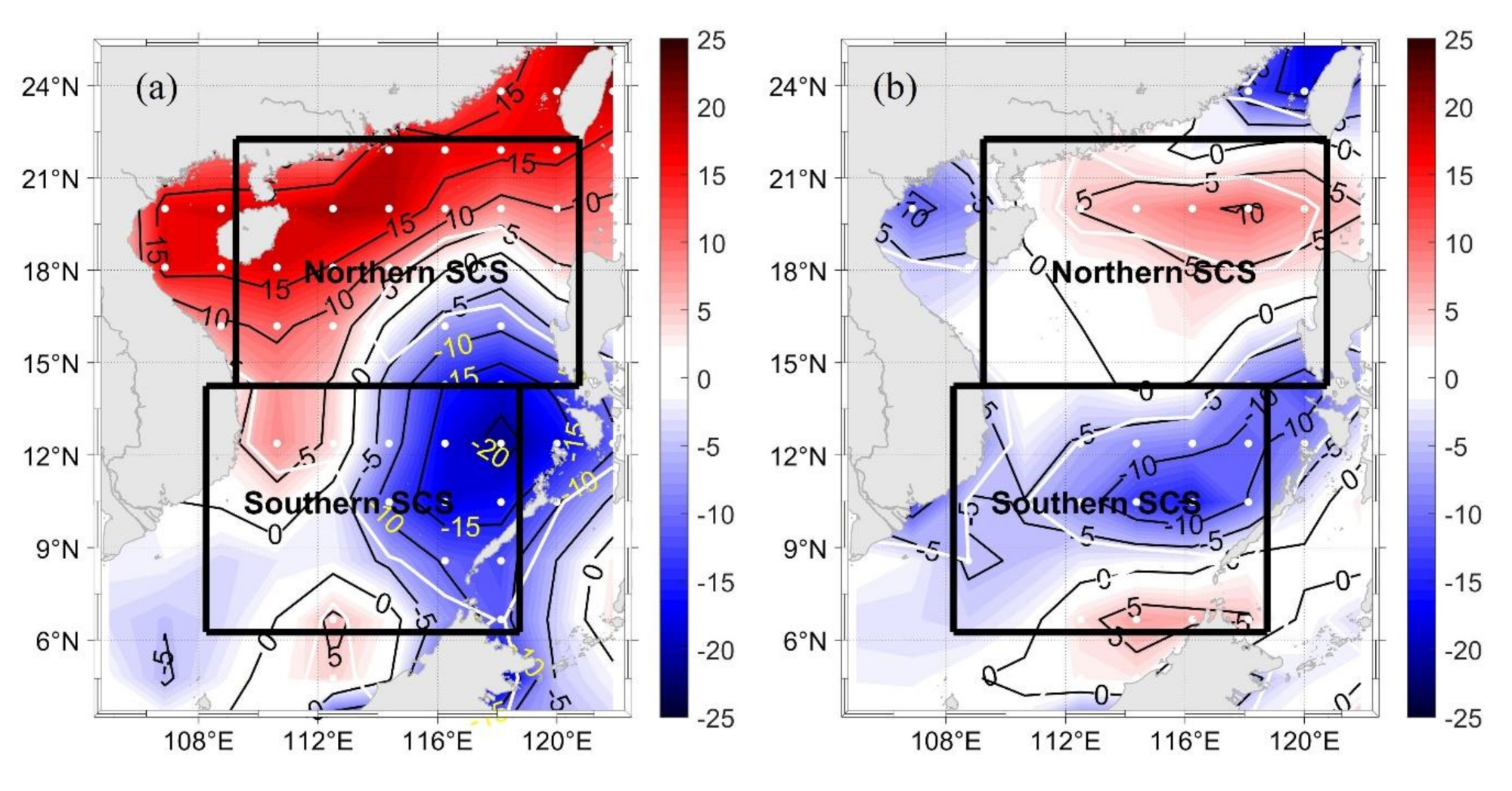
The net heat flux anomalies and latent heat flux anomalies that appeared in El Niño events are researched in this section. Positive heat flux in this paper is defined as the heat that the atmosphere gives to the oceans. As shown in Figure 6a, the composite of net heat flux anomalies during mature winters for EP El Niño exhibits a north–south dipole pattern over the whole SCS. Enhanced (reduced) net heat flux appears in the northern (southern) SCS basin. The maximum value in the North is more than 15 W/m² in the east of Hainan Island, and the minimum value in the South is less than −20 W/m² located in the 118° E, 12° N. 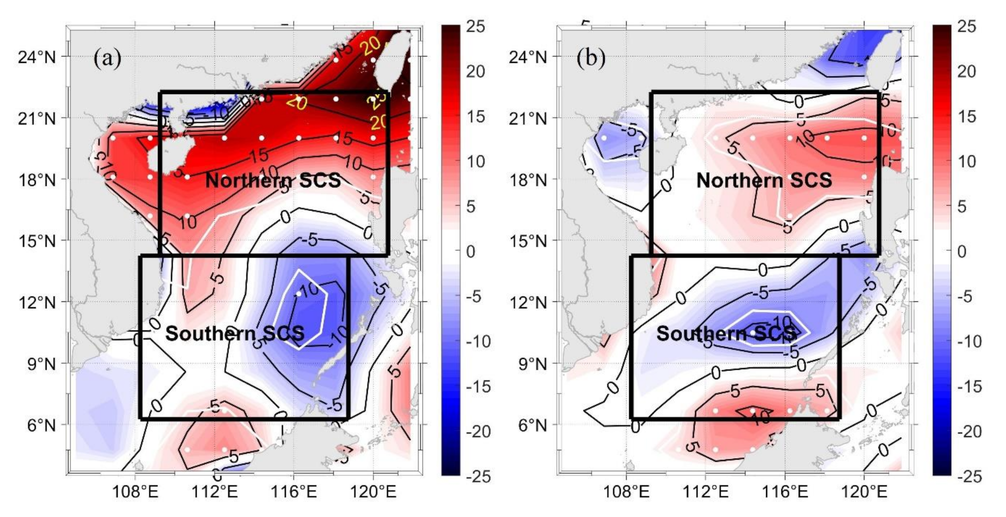As shown in Figure 7a, the anomalous latent heat flux has a similar pattern with the anomalous net heat flux for the EP El Niño. Positive latent heat flux anomalies appear in the northern basin, with a maximum of 25 W/m² to the south of Taiwan Island, and negative latent heat flux anomalies dominate the southern SCS, with a minimum value below −10 W/m² located in the 118° E, 10° N. As for CP El Niño events, the north–south dipole pattern still exists, but the magnitudes of the anomalous net heat flux and anomalous latent heat flux are both smaller than that in the EP El Niño events (Figure 6b and Figure 7b). The similarity of the pattern of latent heat flux anomalies and net heat flux anomalies indicates that the latent flux anomalies are the dominant contributors to the north–south discrepancy of net heat flux anomalies over SCS.

b.

North–South Discrepancy of interannual SCS wind stress anomalies associated with El Niño events.

It is widely recognized that the latent heat flux is greatly affected by 10 m wind speed and air–sea specific humidity difference, which means the anomalous latent heat flux is modulated by large-scale altered atmospheric circulations [13,41]. Indeed, the wind stress over SCS has a north–south discrepant response to El Niño warm SST anomalies, which has been discussed in previous studies. Fang et al. [21] revealed that a remarkable weakening of the northeasterly monsoon emerges during El Niño episode in the northern SCS, but it does not exist over the southern SCS. Lian et al. [35] studied the interannual signal of SCS wind stress anomalies and found that northeastward anomalies prevail in the northern SCS, while southwestward to northwestward anomalies appear in the southern SCS. In this section, an EOF analysis is performed to study the interannual variability contained in the wind stress over SCS in the winter (Figure 8). The first EOF mode explains 82% of its total variance. The spatial distribution of wind stress anomalies in the winter shows a north–south discrepant pattern over SCS, which is similar to that of the composite of SST anomalies in the spring of EP El Niño decaying years (Figure 3a). The amplitude of the wind stress anomalies is significantly stronger over the northern SCS than that over the southern SCS. In this pattern, high wind stress anomalies core exists in 118° E, 20° N, while lower positive wind stress anomalies with westward intensification exist in the southern SCS. As for the direction of wind stress anomalies, there are mainly the southwest wind stress anomalies with larger amplitude in the northern SCS, while mainly the south wind stress anomalies in the southern SCS. The time series of the first EOF mode (not shown) is highly related to the Nino 3 Index (the correlation coefficient is up to 0.57), indicating that the north–south discrepancy of wind stress anomalies is forced by El Niño events.

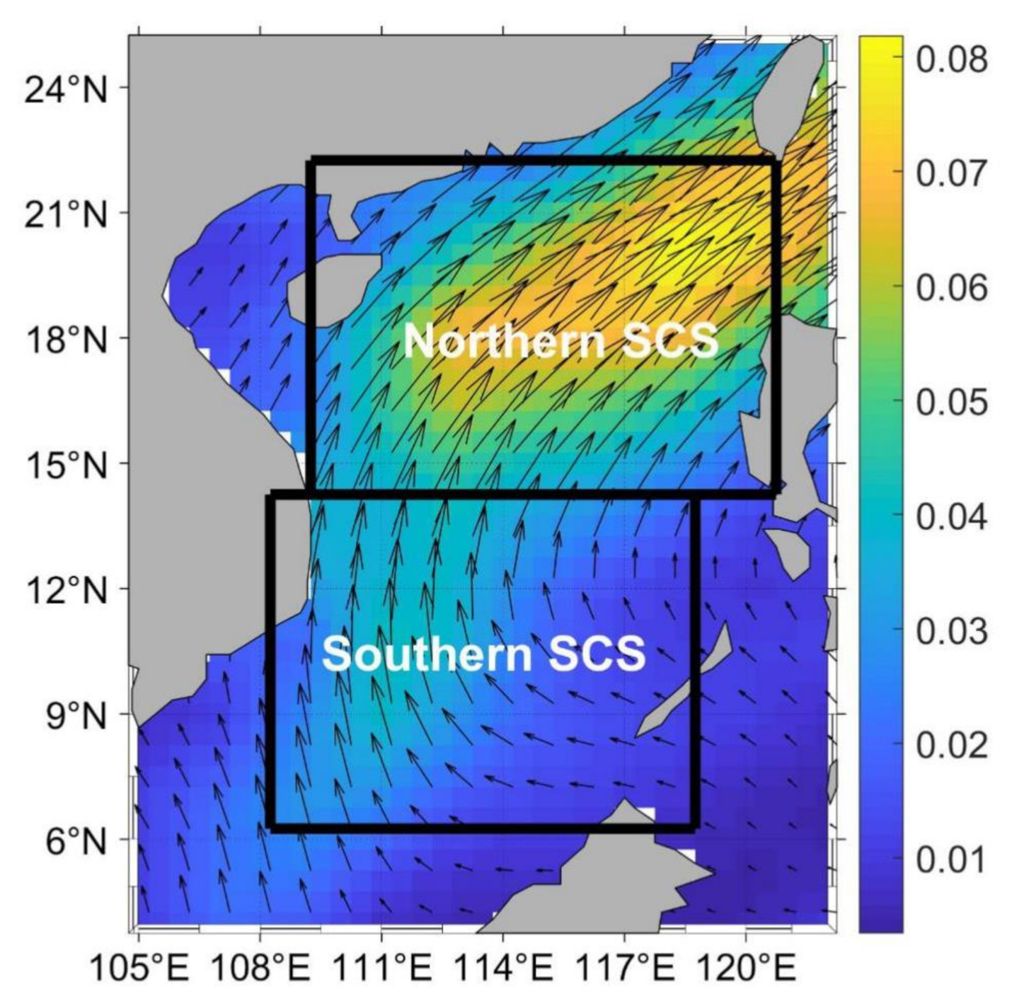
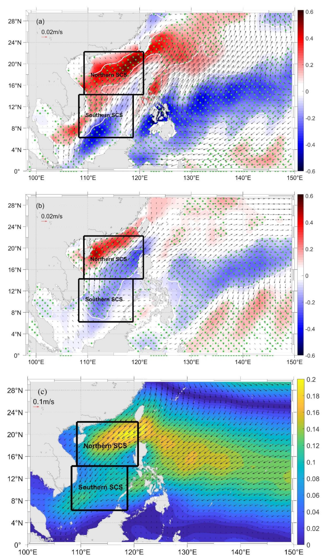
The composite of surface wind stress anomalies and anomalous wind stress curl in winter for EP El Niño and CP El Niño are shown in the Figure 9a,b. The climatological wind stress during winters is shown in Figure 9c. As shown in Figure 9a, in the winters of EP El Niño events, the majority of the SCS is covered by northeastward wind stress anomalies and the highest wind stress anomalies with maximum exceeding 0.035 N/m² are located in the northeast of the SCS deep basin (around 118° E, 20° N, similar location to that mentioned in Figure 8). Specifically, the North is dominated by the southwest wind stress anomalies, and the South is dominated by the south wind stress anomalies. The northern SCS is dominated by the positive anomalous wind stress curl, while the southern SCS is mainly covered by negative anomalous wind stress curl. As shown in Figure 9b, southwest wind stress anomalies prevail in the North with smaller amplitude in the west of Luzon Island than that in Figure 9a and the east to southeast wind stress anomalies prevail in the South. In addition, the region of anomalous positive wind stress curl is compressed to the north boundary of the South China Sea, and the northern SCS is not dominated by the anomalous positive wind stress curl as that in the EP El Niño events. As shown in Figure 9c, the northeast wind stress prevails throughout the SCS.

Extensive research has been made in recent decades to explore the teleconnections between the eastern–Central Pacific and other ocean basins [8,9,10,11,13,14]. Previous papers found that an anomalous low-level anticyclone (cyclone) appears over the western North Pacific during ENSO warm (cold) events [5,9,10,15]. Wang et al. [9] revealed that an anticyclone over the Philippines Sea is the principal center of the massive WNPA, which plays a key role of providing a prolonged ENSO impact on the East Asian climate. The anomalous anticyclone occurs over the tropical Indian Ocean in the summer of El Niño developing years and moves to the SCS in the fall. Then it extends eastward to the Philippine Sea and reaches its peak intensity during the succeeding winter, which maintains through the spring and summer of El Niño decaying years [10,38,42,43]. When the center of WNPA propagates eastward and arrives in the Philippine Sea during the El Niño mature winters, the southwestern portion of anomalous anticyclone dominates the SCS. Thus, it provides anomalous southwesterly wind stress over SCS, which significantly weakens climatological northeasterly wind [9,13,19].

Therefore, the north–south discrepancy of SCS SST anomalies in EP El Niño events is considered to result from the WNPA. The southwest wind stress anomalies in northern SCS greatly offset the northeast climatological wind stress. However, the south wind stress anomalies prevail in the South, and the effect is not as strong as that in the North. The process can be summarized as follows: the WNPA provides southwesterly wind stress anomalies during El Niño mature phases, which weakens the northeasterly monsoon over SCS and results in the north–south discrepancy of anomalous wind stress over SCS. Thus, it in turn leads to the spatial differences of latent heat flux anomalies during the EP El Niño events.

5. Conclusions

Previous research focused on the response of the SST anomalies over the whole SCS basin to ENSO, but the present paper notices the spatial distribution of the response within the SCS basin. The EOF results of the spatiotemporal SST anomalies in spring and the wind stress anomalies in winter are shown in this paper. Both of their first EOF modes show north–south discrepancy, and the time series are highly related to the Nino 3 Index. This north–south discrepant pattern of the first EOF mode of SST anomalies typically appears in the spring. We make composite of SCS SST anomalies in the spring of El Niño decaying years for the EP El Niño events and CP El Niño events, respectively, and find that the discrepancy is only obvious in EP El Niño events, which indicates that the first EOF mode of the SST anomalies mainly reflects the modulation of SCS SST by EP El Niño. The heat budget analysis reveals that net heat flux anomaly forcing is the dominant factor of the SST anomalies tendency in EP El Niño events. We find that the latent heat flux is the major components of the net heat flux over SCS, and the latent heat flux shows positive (negative) anomalies over the northern (southern) SCS, which could be attributed to the north–south discrepancy of wind stress anomalies in both magnitude and direction. Previous research revealed that the El Niño events affect SCS SST through the atmospheric teleconnections. WNPA is considered to play a dominant role in the atmospheric teleconnections, for it provides southwesterly anomalies, and in turn weakens the northeasterly monsoon over the SCS during El Niño mature episodes. Considering the distribution of anomalous wind stress in Figure 8 and Figure 9, we believe that the weakening effect of the anomalous wind stress on northeasterly monsoon is more significant over the northern SCS than the southern SCS.

However, for the CP El Niño, the northern SCS is mainly affected by Ekman heat advection and geostrophic heat advection and the southern SCS is mainly influenced by net surface heat flux anomalies and geostrophic heat advection according to the heat budget analysis, which explains why SST anomalies over SCS do not exist a north–south discrepant pattern, though the wind stress and net (latent) heat flux show some north–south discrepancy to a certain extent.

This paper mainly focuses on the spatial differences of the interannual SCS SST anomalies associated with El Niño. The meridional discrepant performance of interannual variabilities of marine and atmospheric elements discussed above indicate that SCS is likely to have different responses to EP El Niño events between the northern part and southern part. Further experiments with atmospheric and oceanic models to study the responses of other elements over SCS to EP El Niño events are needed to be done. It is worth understanding the full implications of this meridional inhomogeneous response over SCS to ENSO events.