Article

Impacts of Regional Transport and Meteorology on Ground-Level Ozone in Windsor, Canada

1
Department of Civil and Environmental Engineering, University of Windsor, Windsor, ON N9B 3P4, Canada
2
Ontario Ministry of the Environment, Conservation and Parks, Toronto, ON M9P 3V6, Canada
*
Author to whom correspondence should be addressed.
Atmosphere 2020, 11(10), 1111; https://doi.org/10.3390/atmos11101111
Submission received: 17 September 2020 / Revised: 13 October 2020 / Accepted: 15 October 2020 / Published: 16 October 2020
(This article belongs to the Special Issue Tropospheric Ozone Observations)

Abstract

:
This study investigated impacts of regional transport and meteorology on ground-level ozone (O3) in the smog season (April–September) during 1996–2015 in Windsor, Ontario, Canada. Data from five upwind stations in the US, which are within 310 km (i.e., Allen Park and Lansing in Michigan, Erie, National Trail School, and Delaware in Ohio), were included to assess the regional characteristics of O3. The five US stations showed high degrees of similarity with O3 concentrations in Windsor, with overall strong correlations (r = 0.567–0.876 for hourly O3 and r = 0.587–0.92 for 8 h max O3 concentrations) and a low degree of divergence, indicating that O3 pollution in the study area shares regional characteristics. Meteorological conditions played important roles in O3 levels in Windsor. High O3 concentrations were associated with southerly and southwesterly air mass from which polluted and hot air mass was transported and that enhanced local photochemical O3 production. In contrast, northerly flows brought in clean, cool, and dry air mass, and led to low O3 concentrations. Strong correlations were found between numbers of days with 8 h max O3 concentrations greater than 70 ppb and numbers of days with daily max temperature greater than 30 °C, as well as between daily max temperatures and 8 h max O3 concentrations. Nearly half (45%) of the high O3 days (≥90th percentile) occurred in dry tropical weather during 1996–2015, and the 90th percentile 8 h max O3 was associated with dry tropical weather. Occurrences of both southerly flow hours and dry tropical weather type in the smog season increased during the study period. If there were more hot and dry days in the next few decades due to climate change, the effect of emission control on reducing peak O3 values would be diminished. Therefore, continued regional and international efforts are essential to control precursors’ emissions and to mitigate O3 pollution in Windsor.

1. Introduction

Ground-level ozone (O3) is a secondary air pollutant, produced by photochemical reactions between volatile organic compounds (VOC) and nitrogen oxides (NOX) [1]. Both local emissions of O3 precursors and regional transport of O3 and its precursors have strong impacts on O3 levels [1]. O3 production is non-linearly related to levels VOCs and NOX, and mainly depends on the ratio of the two [2,3]. In urban areas where NOX levels are normally high, O3 levels increase with VOC levels but decrease due to the nitric oxide (NO) scavenging effect. At low NOX levels, O3 production is limited by NOX levels but with little impact by VOCs. The degree of O3 scavenging by NO is strongly affected by the ratio of NO to NO2. With the same value of NOX (i.e., NO + NO2), lower NO to NO2 ratios lead to less O3 being consumed [4]. The decreasing ratios of NO to NO2 have been observed in recent years [2,4]. This is one of the reasons that some regions have experienced decreasing NOX but slightly increasing O3 [2].
O3 and its precursors can be transported over several hundred kilometers [5]. Trajectory models, for example, the Hybrid Single Particle Lagrangian Integrated Trajectory (HYSPLIT) [6,7], have been widely used to investigate the impact of airmass movement on air quality [8,9,10] because these models are easy to apply; are often freely available with processed meteorological data; and only require a few input parameters [11]. The back-trajectory analysis is one of the most common model applications to determine the origin of air masses and establish source-receptor relationships [6]. Davis et al. [12] found that high O3 levels in Shenandoah Valley, Virginia, United States (USA) were due to both transport from urban/industrial regions in the Midwest and local photochemical production. Comprehensive models, such as the Community Multi-scale Air Quality (CMAQ) model, have been used to simulate the transport, chemical reactions, and deposition of multiple pollutants simultaneously [13]. A study by Yu et al. [14] investigated photochemical O3 production and total NOX emissions along the 3-day transport path for two sites in the state of New York (USA) in July 2004, and found that O3 concentrations were positively correlated with NOX emissions. Kemball-Cook et al. [15] pointed out that both regional transport and local photochemical production played an important role in the peak O3 levels on exceedance days in the Dallas–Fort Worth (TX, USA) areas in 2002.
Local meteorological conditions also have strong impacts on O3 concentrations, including solar radiation, temperature, cloudiness, and wind speed/direction. A study in Toronto, Ontario reported that on average 16% of variance in O3 concentrations could be explained by midday solar radiation levels during 2008–2012 [16]. Geddes et al. [17] reported (1) a strong association between the number of 65-ppb ozone exceedances and number of days above 30 °C, and (2) summer Ox (O3 + NO2) levels positively correlated with maximum daily temperature (R2 = 0.33) during 2000–2007, in Toronto, Ontario. A study assessed associations between O3 levels and wind directions in Houston (TX, USA) during 1990–2013. The annual number of exceedance days of 1 h O3 was negatively correlated with annual southerly flow (160°–200°) hours at the Aldine (r = −0.63, p < 0.05) and Clinton (r = −0.56, p < 0.05) sites, suggesting clean air mass from the Gulf of Mexico in the south [18].
Besides local weather conditions, O3 concentrations are influenced by large-scale synoptic weather regimes. Synoptic meteorology is associated with large-scale weather-producing disturbances with a horizontal scale of several hundred to a few thousand kilometers, and a lifetime of days [19]. High O3 levels in New York State [8] and in Delaware [20] were found related to transport of O3 and its precursors from upwind states. An evaluation of summertime O3 and six synoptic weather types during 1990–2014 found that high O3 concentrations in Chicago (IL, USA) were strongly associated with dry tropical weather [21]. Associations between elevated O3 levels and synoptic conditions were also found in Washington, DC [22], in the mid-Atlantic [23], and in China [24].
Windsor in Ontario, Canada, is located downwind of several industrial states, including Michigan, Ohio, and Indiana in the US. Local emissions and trans-boundary air pollution led to occasional poor air quality in Windsor [25]. During 1996–2015, concentrations of O3 precursors, i.e., NOX and NMHCs (non-methane hydrocarbons), decreased significantly by 58% and 61%, respectively, in Windsor. However, annual O3 concentrations increased by 33% (20.3 ppb in 1996 vs. 27 ppb in 2015) [2]. The 3-year average (2013–2015) of the annual 4-th highest daily max 8 h O3 was 69 ppb in Windsor, the highest among 21 stations in Ontario [26]. Impacts of NOX and VOCs on O3 long-term trends in Windsor were reported previously [2]. The unique geological conditions in Windsor often lead to southerly and southwesterly air flows from upwind states, especially in summertime. Therefore, there is a need to evaluate to what degree that the higher O3 levels in Windsor comparing to other sites in Ontario are attributable to weather conditions. The objective of this study was to investigate the impacts of regional transport and local/synoptic meteorological conditions on smog season O3 concentrations in Windsor during the 20-year study period of 1996–2015.

2. Methodology

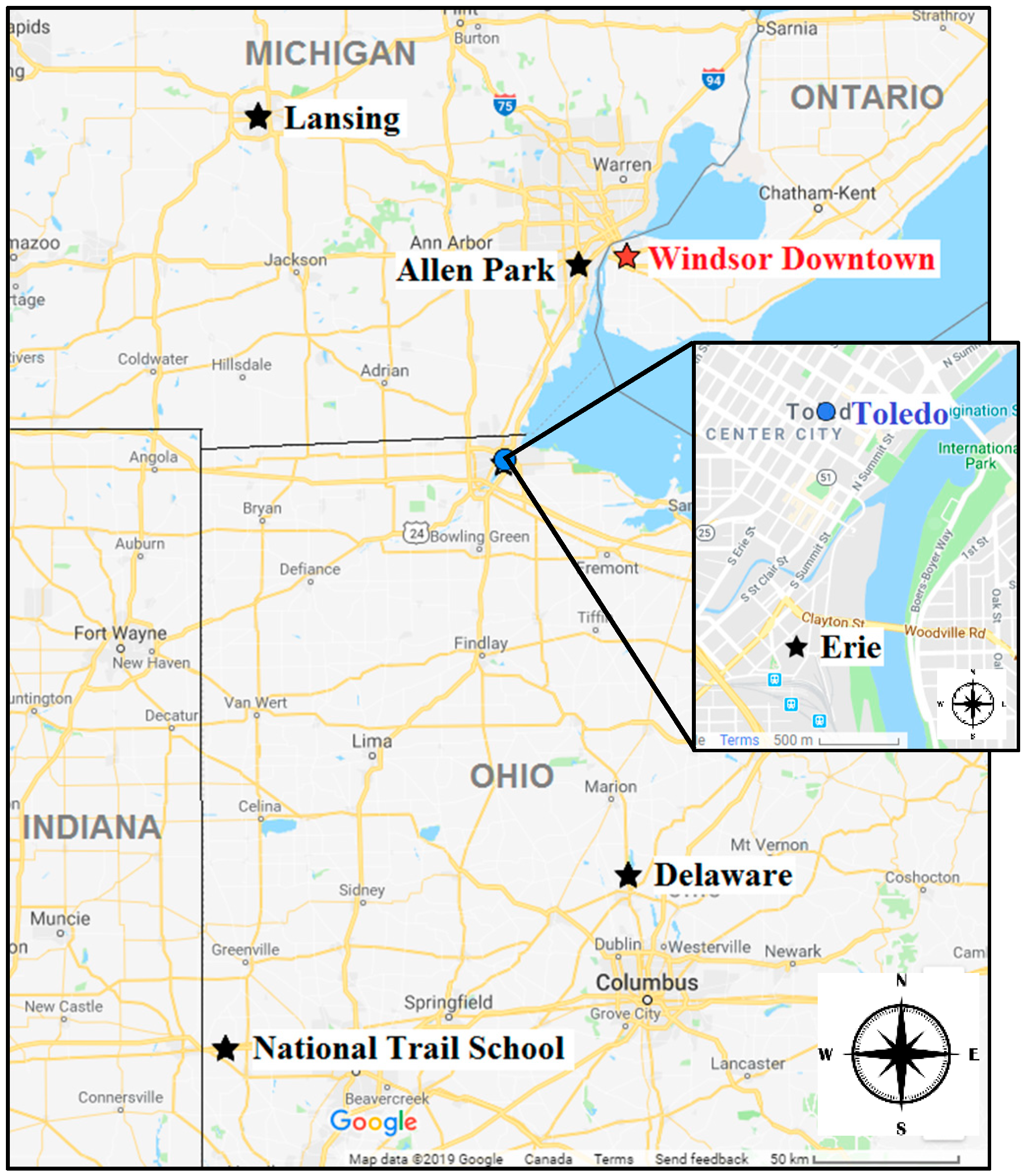
2.1. Data Collection

There are two air quality stations in Windsor (i.e., Windsor Downtown and Windsor West) monitoring O3 among a number of air pollutants [26]. Windsor Downtown (Figure 1) was selected in this study due to a longer period of NO, NO2, and NOX data (1996–2015) than that at Windsor West (2001–2015) as discussed in a companion paper [2].
The prevailing wind direction in Windsor during the 20-year study period was from the southwest (Figure S1). To investigate the regional characteristics of O3, five US O3 monitoring stations located in a range of 17 to 310 km away from Windsor were selected (Figure 1). Two stations (i.e., Allen Park and Lansing) are in Michigan, and the other three stations (i.e., Erie, National Trail School or NTS, and Delaware) are in Ohio. The parameters of each selected station are listed in Table 1.
The smog season in Ontario is from May to September [29], while it varies in the USA (Michigan: April–September; Ohio: April–October). Because monthly mean O3 concentration in April (30 ppb, 1996–2015) was higher than that in September (26 ppb) in Windsor [30], the smog season is defined as from April to September in this study.
Hourly O3 concentrations in Windsor during 1996–2015 were provided by the Ontario Ministry of the Environment, Conservation and Parks (MECP). Smog season hourly O3 concentrations at the five US stations during 1996–2015 were obtained from the United States Environmental Protection Agency (USEPA) website [28]. From the same website, the daily maximum 8 h concentrations for a given calendar day, i.e., the highest of the 24 possible 8 h average concentrations in that day (hereafter referred to as “8 h max O3”) [31] were downloaded for the five US stations during 1996–2015. Hourly meteorological parameters, including temperature, relative humidity, wind direction, wind speed, visibility, atmospheric pressure, and weather conditions (e.g., cloudy, snowy, and clear) at Windsor Airport (8 km southeast from the Windsor Downtown station) during 1996–2015 were downloaded from Environment and Climate Change Canada website [32]. The daily Spatial Synoptic Classification (SSC) data were downloaded from Kent State University website [33]. The SSC method classifies the weather conditions at a given location on a daily basis using surface-based observations, including temperature, dew point, cloud cover, atmospheric pressure, as well as south-north and west-east wind components. The SSC data are available in Windsor and Toledo (Figure 1) during the 20-year study period [33]. Toledo was selected to represent large scale synoptic weather conditions in the study region.
The smog season 8 h max O3 concentrations in Windsor were calculated with hourly O3 concentrations following USEPA’s “Guideline on data handling conventions for the 8 h ozone NAAQS (National Ambient Air Quality Standards)” [31].

2.2. Impact of Airmass Movement on O3 Levels in Windsor

Backward trajectory was used to identify the geographical origins and pathways of air mass arrived in Windsor. Twenty-four-hour backward trajectories in Windsor in each day of the smog season during 1996–2015 were simulated with HYSPLIT [6,7]. The meteorological data are archived Eta Data Assimilation System (EDAS) files with a horizontal resolution of 80 km during 1997–March 2004 and EDAS 40 km during April 2004–2015 [34]. The start time of each trajectory was 15:00 EDT (19:00 UTC) when maximum hourly O3 concentrations normally occurred in a day. The start height of trajectory was 500 m above the ground level to reflect half of the estimated summertime mixing height.
Each backward trajectory was overlaid on a compass with 36-bins in 10° intervals to determine the direction from which the air mass arrived in Windsor. If a 24 h trajectory passed through several 10-degree sectors, only the last segment (18 h–24 h) of the trajectory was used to determine the direction of the air mass. Eight-hour max O3 concentrations by each of the 36-direction of trajectories in smog season were calculated. Hierarchical clustering analysis [35] was used to classify trajectories into three clusters based on the 8 h max O3 concentrations. Meteorological parameters by each cluster were also calculated to investigate the association between 8 h max O3 concentrations and meteorological conditions.

2.3. Impact of Meteorological Parameters on O3 Levels in Windsor

Both local and large-scale synoptic meteorological parameters were used to investigate their impacts on O3 concentrations in Windsor. Spearman’s rank correlation coefficients between hourly O3 concentrations and each meteorological parameter (temperature, relative humidity, visibility, wind speed, and atmospheric pressure) in Windsor were calculated in smog season during the study period. Pearson correlation coefficients between daily mean O3 and meteorological parameters were estimated. Associations between the number of high O3 days (8 h max O3 > 70 ppb) and the number of hot days (daily max temperature >30 °C) in the smog season in each year were assessed. Mean meteorological parameters at high (8 h max O3 > 90th percentile) and low (<10th percentile) O3 days were compared by analysis of variance (ANOVA). Eight-hour max O3 concentrations by three weather types (sunny, cloudy, and rainy days) in the smog season were calculated to investigate the association between 8 h max O3 concentrations and the weather conditions using ANOVA.
SSC was used to investigate the associations in Windsor between 8 h max O3 concentrations in the smog season (April–September) and seven types of weather conditions, dry polar (DP), dry moderate (DM), dry tropical (DT), moist polar (MP), moist moderate (MM), moist tropical (MT), and transitional (TR), as outlined in Jing et al. [21]. Percentage of high O3 days (8 h max O3 >90th percentile) and 8 h max O3 concentrations by each SSC weather pattern were calculated.

2.4. Similarity Analysis

Analysis of similarity among Windsor and the five USA sties was conducted to investigate the regional characteristics of O3 during the study period. The following two methods were employed:
(1)
Spearman’s rank correlation coefficients of smog season hourly O3 concentrations, and Pearson correlation coefficients of smog season daily and monthly O3 concentrations, 8 h max and monthly mean 8 h max O3 concentrations between Windsor and each of the five US sites were calculated.
(2)
Coefficient of divergence (COD, Pinto et al. [36]) of hourly and 8 h max O3 concentrations in the smog season between Windsor and each of the five US sites were calculated as shown in Equation (1):
COD = 1 p i = 1 p ( C i j C i k C i j + C i k ) 2
where p is the total number of paired measurements, and Cij and Cik are the measured concentrations at the j (reference) and k (comparison) sites on the i-th day, respectively. The range of COD values is 0 to 1. Greater COD values indicate spatial heterogeneity of O3 concentrations [37,38].
All analysis outlined in Section 2.2, Section 2.3 and Section 2.4 were carried out in Minitab release 18 (Minitab Inc., State College, PA, USA).

3. Results and Discussion

3.1. General Statistics

Among the six sites, Delaware had the highest 20-year smog season average O3 concentrations (34.6 ppb), followed by Lansing (33.9 ppb), NTS (33.1 ppb), and Windsor (31.7 ppb). The Allen Park and Erie sites registered lower levels (26.7 and 28 ppb, respectively) (Table 2).

3.2. Impact of Weather Conditions on O3 Levels in Windsor

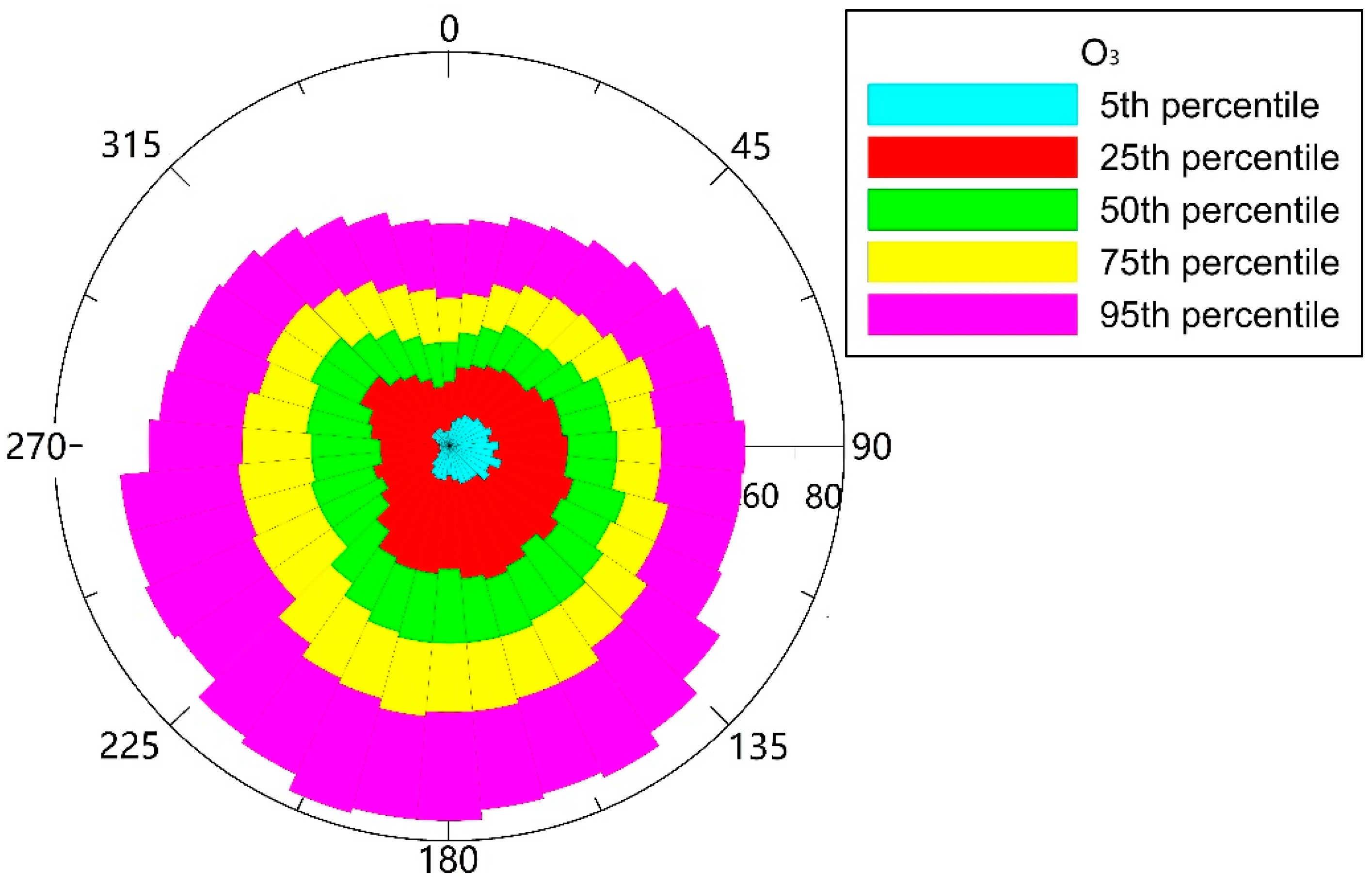
3.2.1. Directional O3 Concentrations

Smog season mean O3 concentrations in Windsor by wind direction are shown in Figure S2. Higher O3 concentrations (39.5 ppb) was associated with air mass from the south and southwest (140°–220°), where several industrial states of the USA are located (e.g., Michigan and Ohio), suggesting regional transport of polluted air mass. Lower O3 concentrations (26 ppb) were associated with winds from the north (320°–50°), suggesting clean air mass from northern Ontario.
Figure 2 depicts distribution of smog season O3 levels in Windsor in each wind direction. Under clean conditions (5th and 25th percentiles), the west and northwesterly flows (230°–360°) are associated with extremely low concentrations in comparison with other directions (2.7 ppb vs. 7.7 ppb for the 5th percentile; 16 ppb vs. 23 ppb for the 25th percentile). For median (50th) and high (75th and 95th) O3 concentrations, southerly flows (140°–220°) bring in significantly more polluted airmass than by flows from the north (330°–20°) (39 ppb vs. 23 ppb for the 50th percentile; 53 ppb vs. 39 ppb for the 75th percentile; 74 ppb vs. 47 ppb for the 95th percentile). Our results further indicate the strong impact of US states on higher O3 levels in Windsor.
As a secondary pollutant, O3 levels depend strongly on regional transport of O3 and precursor concentrations. A study in Texas (USA) investigated impacts of cold front (mainly northerly winds) on area-wide peak levels and regional background concentrations during O3 seasons (April–October) of 2003–2016 [39]. They found that wind direction was the dominant factor causing changes on O3 levels, especially when southerly flow with less anthropogenic emissions from the Gulf of Mexico shifted to northerly flow with more emissions from inland. Plocoste et al. [40] reported strong influences of high O3 levels by meteorological conditions (e.g., wind) in Guadeloupe, a French overseas region located at the Lesser Antilles Arc. The impacts of regional transport from upwind states on high O3 levels have also been reported by other researchers, for example, in the states of New York [8] and Delaware [20].
A USEPA study used the Variable Grid Urban Airshed Model (UAM-V) to determine the pattern of transport in the transboundary region of the eastern United States and Canada [41]. It was found that the magnitude and persistence of high O3 concentrations in eastern North America are strongly influenced by long-range transport of O3 and its precursors. As for transboundary movement of pollutants, more O3 and precursors transport from the US into Canada than from Canada into the USA. Consequently, air mass from the US contributed to high O3 concentrations in Ontario, Quebec, New Brunswick and Nova Scotia, Canada. This is because of higher emissions in the USA and the prevailing winds during the summer O3 season. Commission for Environmental Cooperation reported significant transport of pollutants into southwest Ontario from the upper Midwest US States and the Ohio River Valley [5].
Long-term trend of southerly flow (160°–200°) hours in the smog season in Windsor is shown in Figure 3. The occurrence of southerly flow hours increased in Windsor by 30% (p < 0.05) during the 20-year study period. Furthermore, annual smog season hours of southerly flow were positively correlated with annual smog season O3. The two exceptions are year 2000 and year 2004 with the two lowest annual means (25.5 ppb and 26.6 ppb, respectively), but high in southerly flow hours (638 h and 774 h, respectively) during 1996–2015. The remaining 18 years showed a strong correlation (r = 0.642, p < 0.05). Therefore, increasing southerly flows could be one of the reasons of increasing O3 concentrations in smog season in Windsor reported in Zhang. [30].

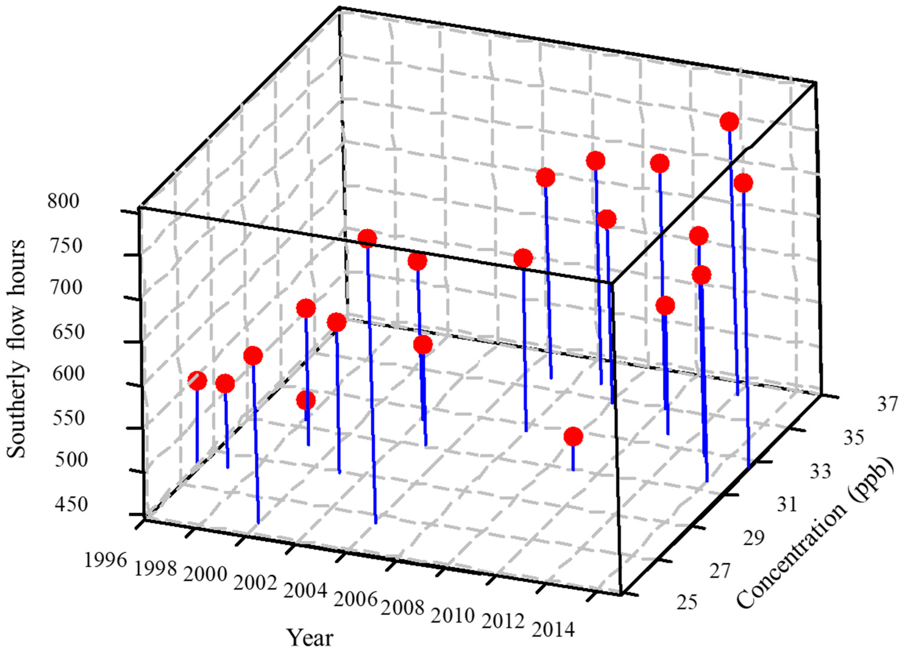
3.2.2. Air Mass Trajectory

Smog season daily 24 h HYSPLIT backward trajectories ending in Windsor during the study period are organized by year in Google Earth format. An example of a backward trajectory plot in 2015 is shown in Figure S3. Backward trajectory plots shared a common feature in each year of the study period, with lower O3 (first quartile, green lines) and higher O3 (forth quartile, red lines) mostly from the north and south, respectively, while the middle levels (second quartile, yellow; third quartile, pink) were from all directions. This once again indicated the impact of regional transport of polluted air mass from the south on higher O3 levels in Windsor.
Smog season 8 h max O3 concentrations averaged by 36 air mass trajectory directions arriving in Windsor during the 20-year study period are shown in Figure S4, the trend is similar to that of the directional concentrations by wind direction (Figure S2) using hourly data. Those 36 directional air trajectories were classified into three clusters. Eight-hour max O3 concentrations by cluster and meteorological conditions of each cluster are summarized in Table 3. One-way ANOVA indicated that there are at least two cluster means of 8 h max O3 concentrations and of each meteorological parameter considered were significantly different from each other (Table S1).
Lower 8 h max O3 concentrations (40.2 ppb) in Windsor were associated with air mass originated from the north of Windsor (300° to 50°, Cluster 1), including northern Michigan and upper Ontario where there are fewer industrial and traffic emission sources. Cluster 1 accounted for 32% of total air mass observed which brought in clear, cool, dry and windy air into Windsor. Strong winds enhanced dispersion of air pollutants, which also lead to low O3 concentrations in Windsor.
Median level 8 h max O3 concentrations (46 ppb) in Windsor were associated with air mass from the east and southeast (60° to 150°, Cluster 2), including Pennsylvania, New York, and Eastern Ohio. Air mass in this cluster is the least frequent (18%) and associated with cool, humid, and slow-moving conditions. The highest percentage of rainy days at 9.3% was found in Cluster 2, suggesting unfavorable conditions for O3 formation.
Eight-hour max O3 concentrations in Cluster 3 were the highest (51 ppb) when air mass was from the south and southwest (160° to 290°) of Windsor, where several industrial states are located including Michigan, western Ohio, Indiana, and southern Illinois. Air mass from Cluster 3 is the most frequent (50%), consistent with prevalent wind direction in Windsor (Figure S1). Air mass in this cluster led to hot days with strong winds. The high temperatures favor photochemical production of O3. Our results suggest that high O3 concentrations in Windsor were caused by both local photochemical production under strong solar radiation and regional transport of O3 and its precursors from the industrial states of the US. Similar findings were reported by other researchers. A study of O3 concentrations in Eastern Canada founded that the elevated levels of warm season O3 are associated with back-trajectories originating from Detroit–Windsor or the Ohio River Valley region [42]. Another O3 modeling study [43] in Southern Ontario in the summer of 2001 reported that around 60% of the O3 formed by anthropogenic emissions in Southern Ontario was due to the emission releases from the nearby US states during the smog episodes.
Among the four meteorological parameters considered in Table 3, temperature and atmospheric pressure are the only two parameters that distinguish Cluster 3 from the other two clusters, while low temperature and relative humidity are unique to Cluster 1 (Table S1). This finding suggests that during the smog season, when hot air mass come from the south and southwest of Windsor, O3 concentration is likely high; while cool and dry air mass from the north tends to lead to lower O3 levels in Windsor.

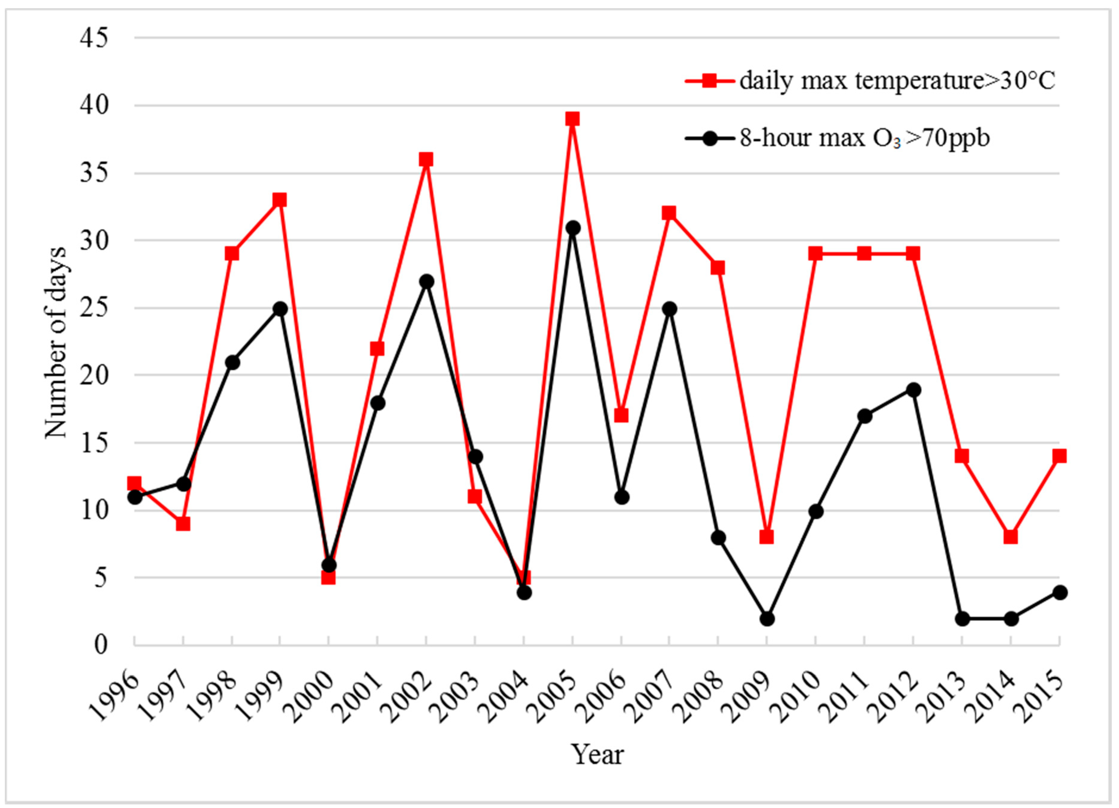
3.2.3. Effects of Meteorological Parameters

Spearman’s rank correlation coefficients and Pearson correlation coefficients between smog season O3 concentrations and five continuous meteorological parameters in Windsor are provided in Table S2. Of the five meteorological parameters investigated, only temperature (hourly data, r = 0.518, p < 0.01) and relative humidity (hourly data, r = −0.521, p < 0.01) were strongly correlated with O3 concentrations during 1996–2015. This suggests faster photochemical production of O3 under warmer and drier conditions [44].
As depicted in Figure 4, the numbers of days of smog season 8 h max O3 greater than 70 ppb was strongly correlated with the numbers of hot days (i.e., daily max temperature greater than 30 °C) in Windsor during the study period (r = 0.833, p < 0.05). Furthermore, there was a strong correlation between daily max temperature and 8 h max O3 concentrations (r = 0.714, p < 0.05) in smog season. This O3 concentration-temperature association is consistent with findings from an O3 study in the Greater Toronto Area of Ontario [17]. Association between elevated O3 levels and high temperatures has also been reported by other studies [3,23,24,40].
Mean meteorological parameters in high (>90th) and low (<10th) smog season 8 h max O3 concentration days are summarized in Table 4. One-way ANOVA and Tukey’s tests indicate that all meteorological parameters were significantly different (p < 0.05) in high and low O3 days, indicating strong influence by weather conditions.
High O3 days (>90th percentile 8 h max O3) were typically associated with high temperature and atmospheric pressure, but low in relative humidity and wind speed. Hot and dry days are generally associated with strong solar intensity, thus enhancing photochemical production of O3 [45]. High pressure and low wind speeds weaken the dispersion and dilution of O3, resulting in high O3 concentrations. The association between light winds and elevated O3 levels was also reported by Johnson et al. [42] in Southern Ontario and Southwest Quebec (Canada) during 1994–2003, and by Davis et al. [12] in Shenandoah Valley of Virginia (USA) during 2001–2006.
Low O3 days (<10th percentile 8 h max O3) were usually accompanied by low temperature and atmospheric pressure, but humid and windy weather. Cooler and humid days are associated with weak solar intensity, thus result in less photochemical production of O3 [45]. Low atmospheric pressure and strong winds enhance dispersion and dilution of O3, leading to low O3 concentrations.
One-way ANOVA also indicates that smog season 8 h max O3 concentrations in clear days (51 ppb) were statistically higher (p < 0.05) than those in cloudy days (45 ppb) and rainy days (33 ppb), which are unfavorable to O3 formation.

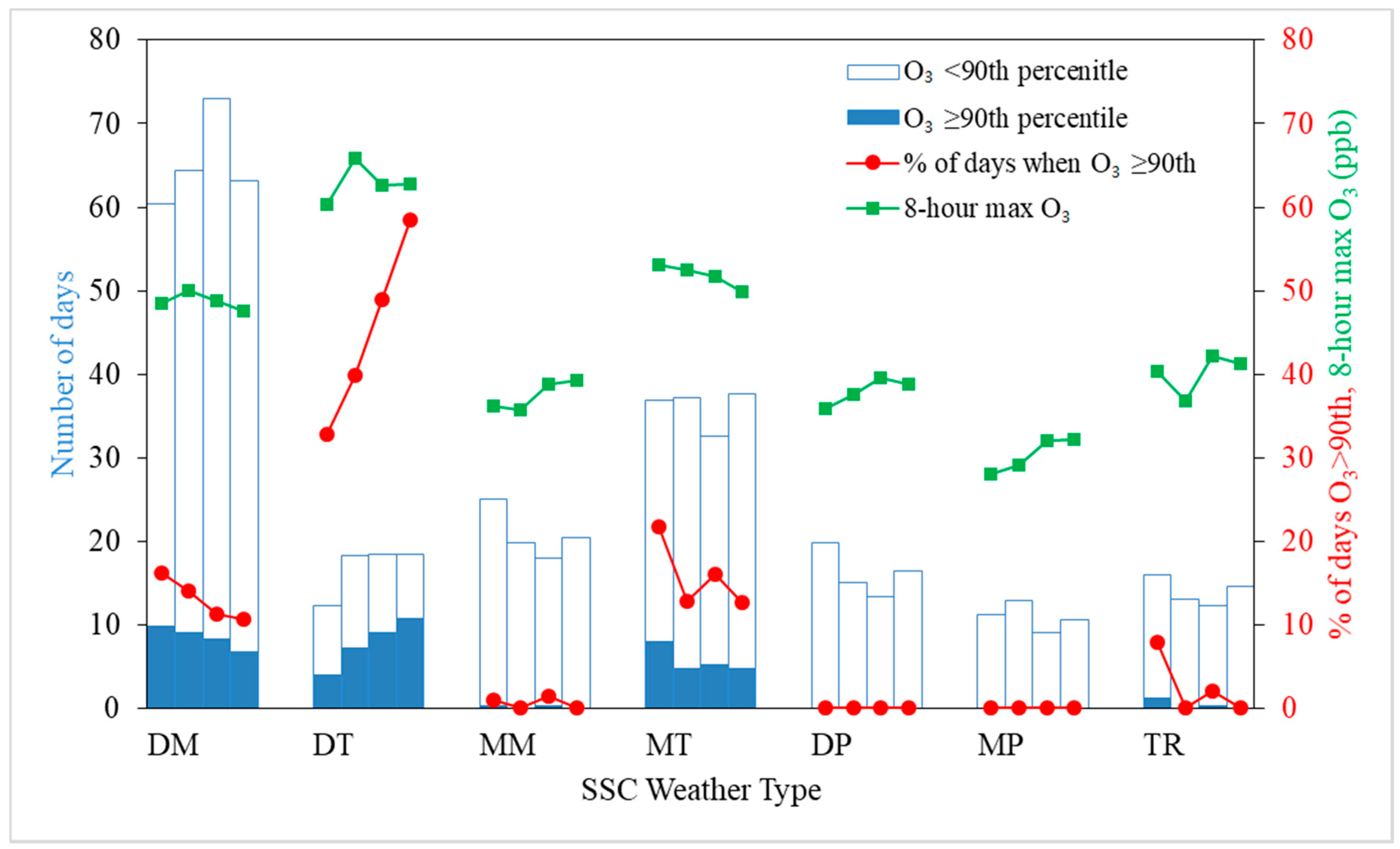
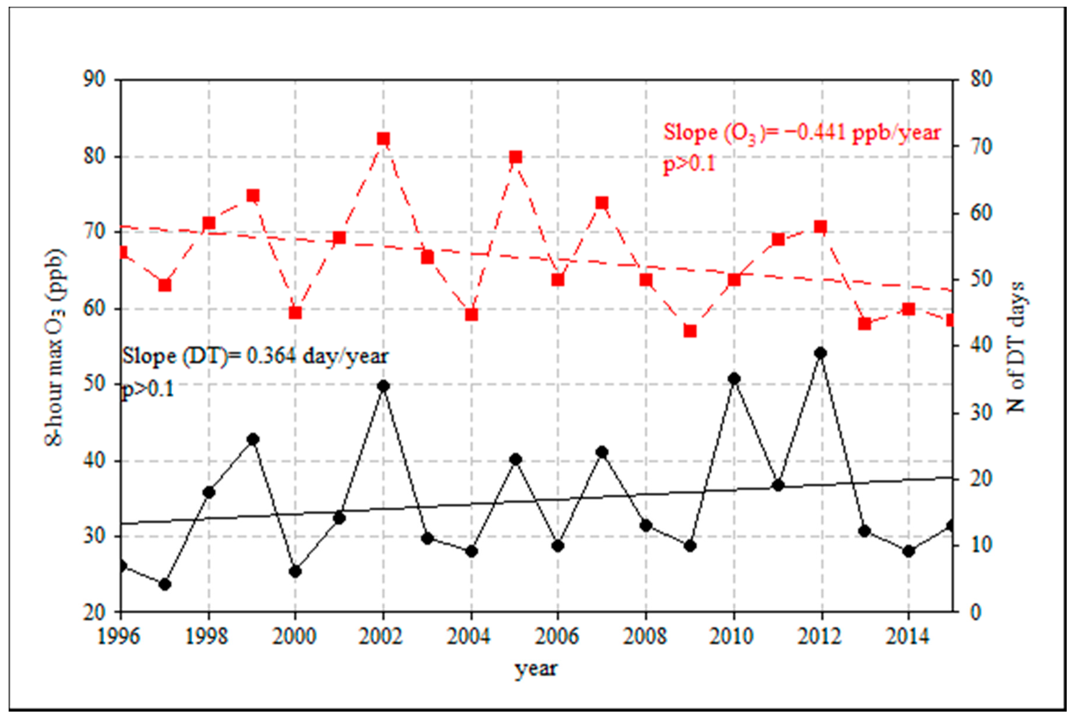
3.2.4. Impact of Synoptic Weather Types

The occurrence frequency of SSC weather types during smog season was calculated for every 5-year period from 1996 to 2015 to assess how it had changed over time, as shown in Figure 5. Warmer weather types (DM, DT, MM, and MT) dominated the study region in comparison with cooler (DP and MP) or transitional (TR) weather types.
The number of high O3 days (8 h max O3 > 90th percentile, shown as solid blue bars in Figure 5) were mainly associated with warm and dry weather types (i.e., DM, DT, and MT), and rarely observed in cool weather types (i.e., DP and MP), high cloudy (MM) or transitional days (TR). The largest number of high O3 days (averaging 8.5 days/yr) was observed under DM weather, primarily because Windsor was influenced by DM weather more often than by other weather types in the smog season. Although DT days were far less frequent than DM and MT days, a high number of high O3 days (7.8 days/yr) was observed under DT weather type. In the past 20 years, high O3 concentrations occurred in nearly half of DT days (45%), much higher than those under the other six weather types (MT 16%, DM 13%, TR 2%, MM 0.6%, DP 0%, and MP 0%). In general, the number of high O3 days decreased or unchanged in all weather types, except for a steady increase in DT weather type.
Trends of DT days and 90th percentile 8 h max O3 during the past 20 years are shown in Figure 6. There was a slight increase in the number of DT days and a marginal decrease in the 90th percentile 8 h max O3 concentration. There was a clear association between these two parameters (r = 0.644, p < 0.05), i.e., annual peak 8 h max O3 values were higher when there were more DT days in that year. If there were more DT days in the next few decades in the study region due to climate change [21], peak O3 concentrations would be increased and the reduction in peak O3 concentrations as the result of emission controls would be diminished.

3.3. Similarity in O3 Concentrations between Windsor and the Five US Sites

3.3.1. Correlation

Table 5 lists correlation coefficients between O3 concentrations in Windsor and at each of the five USA sites during 1996–2015. Strong correlations (r > 0.74) between O3 at Windsor and Allen Park, Erie, and Lansing sites indicate a good agreement in temporal variability of O3 concentrations. Moderate correlation (0.72 > r > 0.4) between O3 at Windsor and NTS as well as Delaware sites suggest less similarity with those two areas which are rural sites and further away from the Windsor (Figure 1). The results of correlation analysis suggest regional characteristics of O3 pollution in the study area. Likewise, correlation coefficients of 8 h max O3 concentrations in the greater Chicago areas (41.3° N–42.6° N, 87.0° W–88.5° W) were calculated during 2005–2013 in the summer months of May to August [38]. The correlation coefficients of 8 h max O3 between any two sites ranged 0.71–0.94, suggesting a similar temporal variability of O3 among the 23 monitoring stations. The lower correlation coefficients were observed at those sites that are furthest apart in the north-south direction.
By examining 8 h max O3 concentrations by cluster, considerately higher correlation coefficients between Windsor and the five USA sites were observed in Cluster 3 (high O3) than in Clusters 1 and 2 (Table 6). This indicates that higher O3 levels associated with southerly and southwesterly flow exhibited a stronger regional signal.

3.3.2. Divergence

As shown in Table 7, the COD values for 8 h max O3 concentrations (0.099–0.148) were lower than those of hourly O3 (0.260–0.338) due to greater spatial variability in the latter. However, COD rankings of O3 concentrations between Windsor and each of the five US sites were consistent in hourly and 8 h max concentrations. O3 concentrations between Windsor and Lansing exhibited the most homogeneity, followed by Allen Park and Erie. Delaware and NTS had less homogeneity with Windsor. This result is largely consistent with the rankings by correlation coefficients (Table 5 and Table 6), once again indicating regional characteristics of O3 in the study area. Other researchers also reported comparable COD values among sites with similar characteristics. A study in Treasure Valley (Idaho, US) estimated COD of O3 concentrations between a reference site (PAR) and six other sites during 1 July to 30 September 2007 [37]. Lower COD values were observed between PAR and two sites (0.06) near downtown Boise, higher COD values between PAR and two sites (0.11–0.17) on the southeast end of the valley, and moderate COD between PAR and two sites (0.08–0.09) located upwind of Boise and influenced by significant mobile sources.

4. Conclusions

This study assessed impacts of regional transport and meteorology on O3 concentrations in Windsor, Canada, by using data collected from 1996–2015. O3 concentrations in the smog season exhibited a high degree of similarity between Windsor and the five USA sites within 310 km, suggesting that the O3 pollution in Windsor and at the five sites in the US showed regional characteristics, likely due to their similar emission sources of O3 precursors and the shared weather conditions.
High O3 concentrations in Windsor were found to be associated with southerly and southwesterly flows that brought in hot and polluted air mass enhancing local photochemical production. In contrast, northerly flows brought in clean, dry and cool air mass from northern Ontario, leading to lower O3 concentrations. Therefore, regional transport of O3 and its precursors from upwind areas had a great impact on O3 levels in Windsor.
Strong correlations were found between numbers of days with 8 h max O3 concentrations greater than 70 ppb and the numbers of days with daily max temperature greater than 30 °C, as well as between daily max temperatures and 8 h max O3 concentrations. The peak O3 (8 h max O3 > 90th percentile) days were associated with hot and calm weather conditions, characterized by high temperature and atmospheric pressure, but low relative humidity and wind speed, belonging to dry tropical weather type, i.e., the hottest and driest synoptic weather conditions.
This study showed that both regional transport and local photochemical production played an important role in the peak O3 levels in smog season in Windsor during the past 20 years. Occurrences of both southerly flow hours and dry tropical weather type in the smog season, which were associated with high 8 h max O3 concentrations, increased during the study period. If there were more hot and dry days in the next few decades due to climate change [3], the effect of emission control on reducing peak O3 values would be diminished. Given increased DT days in the Windsor area, continued regional and international efforts are essential to control precursors’ emissions and to mitigate high O3 levels.

Supplementary Materials

The following are available online at https://www.mdpi.com/2073-4433/11/10/1111/s1, Figure S1. Wind rose in Windsor during 1996–2015, (a) all data, (b) smog season (April to September). Figure S2. Directional smog season mean O3 concentrations in Windsor during 1996–2015. Boxes indicate the interquartile (the 25th to 75th percentile). Middle line in each box represents the median value. The mean value is indicated by a circle marker. Whiskers represent the 1.5 times interquartile ranges. Figure S3. Smog season 24-h backward trajectories arriving in Windsor in 2015. Figure S4. Clustering of smog season 8-h max O3 concentrations averaged by 36 air mass trajectory directions in Windsor during 1996–2015. Table S1. Result of Tukey’s tests of 8-h max O3 and meteorological parameters by cluster in Windsor during 1996–2015 (in Table 3). Table S2. Correlation coefficients between smog season hourly/daily O3 concentrations and meteorological parameters in Windsor during 1996–2015.

Author Contributions

Data collection, data, analysis, visualization, manuscript draft preparation, T.Z.; conceptualization, review and editing of manuscript, X.X. and Y.S. All authors have read and agreed to the published version of the manuscript.

Funding

This project was funded by MECP and the Natural Sciences and Engineering Research Council of Canada.

Acknowledgments

The authors would like to thank all who contributed to collection of air quality data at MECP and ECCC. The authors gratefully acknowledge the NOAA Air Resources Laboratory (ARL) for the provision of the HYSPLIT transport and dispersion model and the READY website (http://www.ready.noaa.gov) used in this publication.

Conflicts of Interest

The authors declare no conflict of interest.

References

  1. Air Quality Expert Group (AQEG). Ozone in the United Kingdom. 2009. Available online: https://uk-air.defra.gov.uk/assets/documents/reports/aqeg/aqeg-ozone-report.pdf (accessed on 6 July 2020).
  2. Xu, X.; Zhang, T.; Su, Y. Temporal variations and trend of ground-level ozone based on long-term measurements in Windsor, Canada. Atmos. Chem. Phys. 2019, 19, 7335–7345. [Google Scholar] [CrossRef] [Green Version]
  3. Lu, X.; Zhang, L.; Shen, L. Meteorology and climate influences on tropospheric ozone: A review of natural sources, chemistry, and transport patterns. Curr. Pollut. Rep. 2019, 5, 238–260. [Google Scholar] [CrossRef] [Green Version]
  4. Akimoto, H.; Mori, Y.; Sasaki, K.; Nakanishi, H.; Ohizumi, T.; Itano, Y. Analysis of monitoring data of ground-level ozone in Japan for long-term trend during 1990–2010: Causes of temporal and spatial variation. Atmos. Environ. 2015, 102, 302–310. [Google Scholar] [CrossRef]
  5. Commission for Environmental Cooperation (CEC). Long-Range Transport of Ground Level Ozone and Its Precursors: Assessment of Methods to Quantify Transboundary Transport within the Northeastern United States and Eastern Canada. 1997. Available online: http://www3.cec.org/islandora/en/item/2185-long-range-transport-ground-level-ozone-and-its-precursors-en.pdf (accessed on 6 July 2020).
  6. Stein, A.F.; Draxler, R.R.; Rolph, G.D.; Stunder, B.J.B.; Cohen, M.D.; Ngan, F. NOAA’s HYSPLIT atmospheric transport and dispersion modeling system. Bull. Amer. Meteorol. Soc. 2015, 96, 2059–2077. [Google Scholar] [CrossRef]
  7. Rolph, G.; Stein, A.; Stunder, B. Real-time environmental applications and display system: READY. Environ. Model. Softw. 2017, 95, 210–228. [Google Scholar] [CrossRef]
  8. Aleksic, N.; Kent, J.; Walcek, C. On ground truth in cross-border ozone transport. J. Air Waste Manag. Assoc. 2019, 69, 977–987. [Google Scholar] [CrossRef]
  9. Lei, R.; Talbot, R.; Wang, Y.; Wang, S.; Estes, M. Surface MDA8 ozone variability during cold front events over the contiguous United States during 2003–2017. Atmos. Environ. 2019, 213, 359–366. [Google Scholar] [CrossRef]
  10. Stroud, C.; Ren, S.; Zhang, J.; Moran, M.; Akingunola, A.; Makar, P.; Munoz-Alpizar, R.; Leroyer, S.; Bélair, S.; Sills, D.; et al. Chemical analysis of surface-level ozone exceedances during the 2015 Pan American Games. Atmosphere 2020, 11, 572. [Google Scholar] [CrossRef]
  11. Pérez, I.A.; Artuso, F.; Mahmud, M.; Kulshrestha, U.; Sánchez, M.L.; García, M.A. Applications of air mass trajectories. Adv. Meteorol. 2015. [Google Scholar] [CrossRef]
  12. Davis, R.E.; Normile, C.P.; Sitka, L.; Hondula, D.M.; Knight, D.B.; Gawtry, S.P.; Stenger, P.J. A comparison of trajectory and air mass approaches to examine ozone variability. Atmos. Environ. 2010, 44, 64–74. [Google Scholar] [CrossRef]
  13. Fu, J.S.; Streets, D.G.; Jang, C.J.; Hao, J.; He, K.; Wang, L.; Zhang, Q. Modeling regional/urban ozone and particulate matter in Beijing, China. J. Air Waste Manag. 2009, 59, 37–44. [Google Scholar] [CrossRef] [PubMed]
  14. Yu, S.; Mathur, R.; Kang, D.; Schere, K.; Tong, D. A study of the ozone formation by ensemble back trajectory-process analysis using the Eta-CMAQ forecast model over the Northeastern U.S. during the 2004 ICARTT period. Atmos. Environ. 2009, 43, 355–363. [Google Scholar] [CrossRef]
  15. Kemball-Cook, S.; Parrish, D.; Ryerson, T.; Nopmongcol, U.; Johnson, J.; Tai, E.; Yarwood, G. Contributions of regional transport and local sources to ozone exceedances in Houston and Dallas: Comparison of results from a photochemical grid model to aircraft and surface measurements. J. Geophys. Res. 2009, 114, 1–14. [Google Scholar] [CrossRef] [Green Version]
  16. Pugliese, S.; Murphy, J.; Geddes, J.; Wang, J. The impacts of precursor reduction and meteorology on ground-level ozone in the Greater Toronto Area. Atmos. Chem. Phys. 2014, 14, 8197–8207. [Google Scholar]
  17. Geddes, J.A.; Murphy, J.G.; Wang, D.K. Long term changes in nitrogen oxides and volatile organic compounds in Toronto and the challenges facing local ozone control. Atmos. Environ. 2009, 43, 3407–3415. [Google Scholar] [CrossRef]
  18. Liu, L.; Talbot, R.; Lan, X. Influence of climate change and meteorological factors on Houston’s air pollution: Ozone a case study. Atmosphere 2015, 6, 623–640. [Google Scholar] [CrossRef] [Green Version]
  19. Reynolds, R. Synoptic meteorology—Weather maps. In Encyclopedia of Atmospheric Sciences, 2nd ed.; North, G.R., Pyle, J., Zhang, F., Eds.; Academic Press: Cambridge, MA, USA, 2015; pp. 289–298. [Google Scholar]
  20. Moghani, M.; Archer, C.; Mirzakhalili, A. The importance of transport to ozone pollution in the U.S. Mid-Atlantic. Atmos. Environ. 2018, 191, 420–431. [Google Scholar] [CrossRef]
  21. Jing, P.; O’Brien, T.; Streets, D.G.; Patel, M. Relationship of ground-level ozone with synoptic weather conditions in Chicago. Urban Clim. 2016, 17, 161–175. [Google Scholar] [CrossRef]
  22. Oyola, M.; Schneider, A.; Campbell, J.; Joseph, E. Meteorological influences on tropospheric ozone over suburban Washington, DC. Aerosol Air Qual. Res. 2018, 18, 1168–1182. [Google Scholar] [CrossRef] [Green Version]
  23. Archer, C.; Brodie, J.; Rauscher, S. Global warming will aggravate ozone pollution in the U.S. mid-Atlantic. J. Appl. Meteor. Climatol. 2019, 58, 1267–1278. [Google Scholar] [CrossRef]
  24. Han, H.; Liu, J.; Shu, L.; Wang, T.; Yuan, H. Local and synoptic meteorological influences on daily variability in summertime surface ozone in eastern China. Atmos. Chem. Phys. 2020, 20, 203–222. [Google Scholar] [CrossRef] [Green Version]
  25. Ministry of the Environment (MOE). Transboundary Air Pollution in Ontario; PIBS 5158e: Toronto, ON, Canada, 2005. Available online: http://www.airqualityontario.com/downloads/TransboundaryAirPollutionInOntario2005.pdf (accessed on 27 July 2020).
  26. Ministry of the Environment and Climate Change (MOECC). Air Quality in Ontario 2015 Report; Queen’s Printer for Ontario: Toronto, ON, Canada, 2017; ISSN 1710-8136. Available online: http://www.airqualityontario.com/downloads/AirQualityInOntarioReportAndAppendix2015.pdf (accessed on 27 July 2020).
  27. Ministry of the Environment, Conservation and Parks (MECP). Windsor Downtown: Station Information. 2020. Available online: http://www.airqualityontario.com/history/station.php?stationid=12008 (accessed on 6 July 2020).
  28. United States Environmental Protection Agency (USEPA). Pre-Generated Data Files. 2020. Available online: https://aqs.epa.gov/aqsweb/airdata/download_files.html (accessed on 6 July 2020).
  29. Ministry of the Environment (MOE). Air Quality in Ontario Report for 2011; Queen’s Printer for Ontario, PIBS 9196e: Toronto, ON, Canada, 2013. Available online: http://www.airqualityontario.com/downloads/AirQualityInOntarioReportAndAppendix2011.pdf (accessed on 27 July 2020).
  30. Zhang, T. Long-Term Trend of Ground-Level Ozone through Statistical and Regional Transport Analysis. Master’s Thesis, University of Windsor, Windsor, ON, Canada, 2016. Available online: http://scholar.uwindsor.ca/etd/5880/ (accessed on 15 October 2020).
  31. United States Environmental Protection Agency (USEPA). Guideline on Data Handling Conventions for the 8-h Ozone NAAQS, Research Triangle Park, NC. 1998. Available online: https://www3.epa.gov/ttn/naaqs/aqmguide/collection/cp2_old/19981201_oaqps_epa-454_r-99-017.pdf (accessed on 6 July 2020).
  32. Environment and Climate Change Canada (ECCC). Historical Climate Data. 2020. Available online: http://climate.weather.gc.ca/index_e.html (accessed on 6 July 2020).
  33. Kent State University (KSU). Spatial Synoptic Classification. 2020. Available online: http://sheridan.geog.kent.edu/ssc.html (accessed on 6 July 2020).
  34. National Oceanic and Atmospheric Administration (NOAA). What Are the Differences between EDAS, GDAS, FNL, REANALYSIS, and NGM Meteorological Datasets? 2020. Available online: https://www.ready.noaa.gov/faq_md3.php (accessed on 15 May 2020).
  35. Barrado, A.L.; García, S.; Barrado, E.; Pérez, R.M. PM2.5-bound PAHs and hydroxy-PAHs in atmospheric aerosol samples: Correlations with season and with physical and chemical factors. Atmos. Environ. 2012, 49, 224–232. [Google Scholar] [CrossRef]
  36. Pinto, J.P.; Lefohn, A.S.; Shadwick, D.S. Spatial variability of PM2.5 in urban areas in the United States. J. Air Waste Manag. Assoc. 2004, 54, 440–449. [Google Scholar] [CrossRef] [PubMed] [Green Version]
  37. Kavouras, I.G.; DuBois, D.W.; Etyemezian, V.; Nikolich, G. Spatiotemporal variability of ground level ozone and influence of smoke in Treasure Valley, Idaho. Atmos. Res. 2013, 124, 44–52. [Google Scholar] [CrossRef]
  38. Jing, P.; Lu, Z.; Xing, J.; Streets, D.G.; Tan, Q.; O’Brien, T. Response of the summertime ground level ozone trend in the Chicago area to emission controls and temperature changes, 2005–2013. Atmos. Environ. 2014, 99, 630–640. [Google Scholar] [CrossRef]
  39. Lei, R.; Talbot, R.; Wang, Y.; Wang, S.C.; Estes, M. Influence of cold fronts on variability of daily surface O3 over the Houston-Galveston-Brazoria area in Texas USA during 2003–2016. Atmosphere 2018, 9, 159. [Google Scholar] [CrossRef] [Green Version]
  40. Plocoste, T.; Dorville, J.-F.; Monjoly, S.; Jacoby-Koaly, S.; André, M. Assessment of nitrogen oxides and ground-level ozone behavior in a dense air quality station network: Case study in the Lesser Antilles Arc. J. Air Waste Manag. Assoc. 2018, 68, 1278–1300. [Google Scholar] [CrossRef] [Green Version]
  41. United States Environmental Protection Agency (USEPA). Ground Level Ozone: Occurrence and Transport in Eastern North America. 1999. Available online: https://www.epa.gov/sites/production/files/2015-07/documents/ground-level_ozone_occurrence_and_transport_in_eastern_north_america.pdf (accessed on 18 May 2020).
  42. Johnson, D.; Mignacca, D.; Herod, D.; Jutzi, D.; Miller, H. Characterization and identification of trends in average ambient ozone and particulate matter levels through trajectory cluster analysis in Eastern Canada. J. Air Waste Manag. Assoc. 2007, 57, 907–918. [Google Scholar] [CrossRef]
  43. Gálvez, O. Synoptic-scale transport of ozone into Southern Ontario. Atmos. Environ. 2007, 41, 8579–8595. [Google Scholar] [CrossRef]
  44. Susaya, J.; Kim, K.H.; Shon, Z.H.; Brown, R.J. Demonstration of long-term increases in tropospheric O3 levels: Causes and potential impacts. Chemosphere 2013, 92, 1520–1528. [Google Scholar] [CrossRef]
  45. Shan, W.; Yin, Y.; Lu, H.; Liang, S. A meteorological analysis of ozone episodes using HYSPLIT model and surface data. Atmos. Res. 2009, 93, 767–776. [Google Scholar] [CrossRef]
Figure 1. O3 monitoring at Windsor (red star) and five USA sites (black star) and a weather station in Toledo (blue circle) (base maps adapted from Google Maps, coordinates of monitoring sites from the Ontario Ministry of the Environment, Conservation and Parks (MECP) [27] and United States Environmental Protection Agency (USEPA) [28]).
Atmosphere 11 01111 g001
Figure 2. Ozone pollution rose in Windsor during the smog season of 1996–2015.
Atmosphere 11 01111 g002
Figure 3. Annual O3 concentration (Y-axis) and number of southerly flow hours (Z-axis) in Windsor during the smog season of 1996–2015.
Atmosphere 11 01111 g003
Figure 4. Number of days of smog season 8 h max O3 greater than 70 ppb and number of daily max temperature greater than 30 °C in each year in Windsor during 1996–2015.
Atmosphere 11 01111 g004
Figure 5. Occurrence frequency of different spatial synoptic classification (SSC) weather types and 8 h max O3 in Windsor in smog season during 1996–2015. DM (dry moderate), DT (dry tropical), MM (moist moderate), MT (moist tropical), DP (dry polar), MP (moist polar), and TR (transitional). Each bar or point represents a period of 5-year.
Atmosphere 11 01111 g005
Figure 6. Smog season 90th percentile 8 h max O3 concentrations in Windsor and the number of dry tropical (DT) days during 1996–2015.
Atmosphere 11 01111 g006
Table 1. Parameters of selected monitoring sites. Data source: Windsor station from MECP [27], five US sites from USEPA [28].
Site NameProvince/StatesLatitude (Degree)Longitude (Degree)Elevation above Sea Level (m)Site TypeDistance to Windsor (km)Data Availability
Windsor DowntownOntario42.31−83.04176Urban-1996–2015
Allen ParkMichigan42.22−83.20181Suburban171996–2015
LansingMichigan42.73−84.53268Urban1301996–2015
ErieOhio41.64−83.54176Urban851998–2015
DelawareOhio40.35−83.06275Rural2181996–2015
National Trail SchoolOhio39.83−84.72357Rural3101997–2015
Table 2. General statistics of smog season O3 concentrations (ppb) at Windsor and five US sites during 1996–2015. SD stands for standard deviation. CV stands for coefficient of variation (SD/mean * 100%).
SitesMeanSDCV (%)5th Percentile25th PercentileMedian75th Percentile95th PercentileMaxSample Size
Windsor31.718.257.541930436412885,259
Allen Park26.718.468.611226395912383,998
Erie28.017.963.821427405912175,998
Lansing33.916.949.962233456311085,693
Delaware34.619.355.842034486816179,203
NTS33.118.455.522033466412186,811
Table 3. Smog season meteorological parameters and 8 h max O3 concentrations in Windsor during 1996–2015 in the three clusters.
Cluster (Air Mass Direction)8 h Max O3 (ppb)Number of DaysDaily Mean Temp (°C)Daily Mean Relative Humidity (%)Daily Mean Wind Speed (km/h)Daily Mean Atmospheric Pressure (kPa)Percentage of Rainy Days (%)
1 (300°–50°)40.2113416.566.314.199.34.3
2 (60°–150°)45.961416.468.212.499.69.3
3 (160°–290°)51.0175219.868.014.699.24.7
Table 4. Meteorological parameters in smog season high O3 (>90th percentile 8 h max O3), low O3 (<10th percentile 8 h max O3), and all days in Windsor during 1996–2015.
DaySample Size8 h Max O3 (ppb)Daily Max Temp (°C)Daily Mean Temp (°C)Daily Mean Relative Humidity (%)Daily Mean Wind Speed (km/h)Daily Mean
Atmospheric
Pressure (kPa)
High O336674.629.423.763.511.599.4
Low O336624.117.814.474.81599.2
All366046.622.918.167.514.199.3
Table 5. Correlation coefficients between smog season O3 concentrations at Windsor and each of the five US sites. All correlations are significant at p < 0.05.
SitesHourly O38 h Max O3Rank
Hourly aDaily Mean bMonthly Mean bDaily bMonthly Mean b
Allen Park0.8760.8940.8900.9200.9111
Erie0.7660.7490.7560.8240.8233
Lansing0.7780.8170.8360.8270.8472
Delaware0.6890.5880.5540.6940.7154
NTS0.5670.4080.6530.5870.6765
a: Spearman’s correlation coefficients. b: Pearson correlation coefficients.
Table 6. Pearson correlation coefficients between smog season 8 h max O3 at Windsor and each of the five US sites by cluster (see Table 3). All correlations are significant at p < 0.05.
SiteCluster 3 (160°–290°, N = 1752)Clusters 1 and 2 (300°–150°, N = 1748)Rank
Allen Park0.9360.8971
Eire0.8490.8062
Lansing0.8340.8013
Delaware0.7070.6064
NTS0.6350.5285
Table 7. Coefficient of divergence (COD) of smog season O3 concentrations between Windsor and each of the five USA sites during 1996–2015.
SitesHourly O38 h Max O3Rank
Allen Park0.2730.1062
Erie0.2910.1183
Lansing0.2600.0991
Delaware0.3020.1364
NTS0.3380.1485
Publisher’s Note: MDPI stays neutral with regard to jurisdictional claims in published maps and institutional affiliations.

