Increasing Neurons or Deepening Layers in Forecasting Maximum Temperature Time Series?

Abstract

Weather forecasting, especially that of extreme climatic events, has gained considerable attention among researchers due to their impacts on natural ecosystems and human life. The applicability of artificial neural networks (ANNs) in non-linear process forecasting has significantly contributed to hydro-climatology. The efficiency of neural network functions depends on the network structure and parameters. This study proposed a new approach to forecasting a one-day-ahead maximum temperature time series for South Korea to discuss the relationship between network specifications and performance by employing various scenarios for the number of parameters and hidden layers in the ANN model. Specifically, a different number of trainable parameters (i.e., the total number of weights and bias) and distinctive numbers of hidden layers were compared for system-performance effects. If the parameter sizes were too large, the root mean square error (RMSE) would be generally increased, and the model’s ability was impaired. Besides, too many hidden layers would reduce the system prediction if the number of parameters was high. The number of parameters and hidden layers affected the performance of ANN models for time series forecasting competitively. The result showed that the five-hidden layer model with 49 parameters produced the smallest RMSE at most South Korean stations.

1. Introduction

An artificial neural network (ANN) is a system for information processing inspired by biological neural networks. The key element of this network is the huge amount of highly interconnected processing nodes (neurons) that work together by a dynamic response to process the information. A neural network is useful for modeling the non-linear relation between the input and output of a system [1]. Compared to other machine learning methods such as autoregressive moving averages (ARMA), autoregressive integrated moving averages (ARIMA), and random forest (RF), the ANN model showed better performance in regression prediction problems [2,3,4]. According to Agrawal [5], the ANN model predicted rainfall events more accurately than the ARIMA model. In another work, ANNs have been applied to forecast monthly mean daily global solar radiation [6].

Furthermore, the ANN model has also been employed to forecast climatological and meteorological variables. Although it is known that the weather forecasting problem is challenging because of its chaotic and dynamic process, weather forecasting based on ANNs has been employing considerably in recent years due to the success of the ANN’s ability. From some previous research, artificial neural networks have been shown as a promising method to forecast weather and time series data due to their capability of pattern recognition and generalization [7,8]. Smith et al. [9] developed an improved ANN to forecast the air temperature from 1 to 12 h ahead by increasing the number of samples in the training, adding additional seasonal variables, extending the duration of prior observations, and varying the number of hidden neurons in the network. Six hours of prior data were chosen as the inputs for the temperature prediction since a network with eight prior observations performed worse than the six hour network. Moreover, it is demonstrated that the models using one hidden layer with 40 neurons performed better than other models over repeated instantiations. In another study, the ANN models for the maximum as well as minimum temperature, and relative humidity forecasting were proposed by Sanjay Mathur [10] using time series analysis. The multilayer feedforward ANN model with a back-propagation algorithm was used to predict the weather conditions in the future, and it was found that the forecasting model could make a highly accurate prediction. The authors in [11] employed the ANN models to forecast air temperature, relative humidity, and soil temperature in India, showing that the ANN model was a robust tool to predict meteorological variables as it showed promising results with 91–96% accuracy for predictions of all cases. In this study, we also aimed to predict the air temperature one day ahead of past observations using the ANN model.

The effectiveness of a network-based approach depends on the architecture of the network and its parameters. All of these considerations are complex, and the configuration of a neural network structure depends on the problem [12]. If unsuitable network architecture and parameters are selected, the results may be undesirable. On the other hand, a proper design of network architecture and parameters can produce desirable results [13,14]. However, little investigation has been conducted on the effect of parameters and architecture on the model’s performance. The selection of ANN architecture, consisting of input variables, the number of neurons in the hidden layer, and the number of hidden layers is a difficult task, so the structure of the network is usually determined by a trial and error approach and based on the experience of the modeler [5]. In another previous study, we compared one-hidden layer and multi-hidden layer ANN models in maximum temperature prediction at five stations in South Korea [15]. In addition, the genetic algorithm was applied to find the best architecture of models. It showed that the ANN with one hidden layer performed the most accurate forecasts. However, the effect of the number of hidden layers and neurons on the ANN’s performance in the maximum temperature time series prediction is not sufficient. It may expect that the model performs worse when the number of parameters decreases. However, what happens if we further increase the number of tunable parameters? There are two competing effects. On the one hand, more parameters, which mean more neurons, become available, possibly allowing for better predictions. On the other hand, the higher the parameter number, the more overfitting the model is. Will the networks be robust if more trainable parameters than necessary are present? Is a one-hidden layer model always better than a multi-hidden layer model for maximum temperature forecasting in South Korea? Therefore, it is also apparently several problems related to the model proper architecture.

This paper proposed a new strategy that applied the ANNs using different learning parameters and hidden layers to empirically compare the prediction performance of daily maximum temperature time series. This study aimed to discuss the effect of parameters on the performance of ANN for temperature time series forecasting.

The rest of the paper is structured as follows. Section 2 describes the data and methodology used for the experiments. Section 3 describes the results, and the final section provides conclusions and directions for future work.

2. Data and Methods

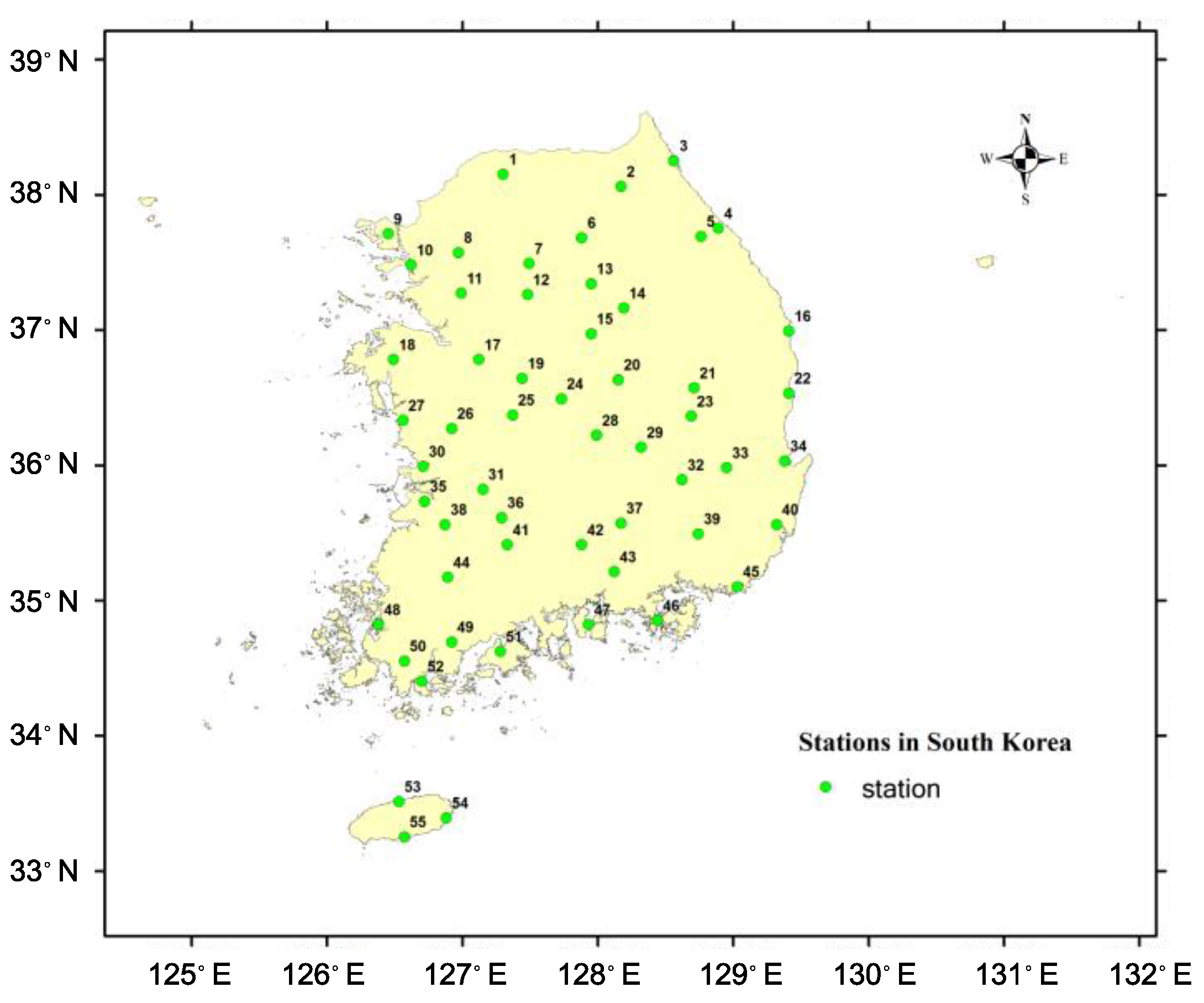
In the current study, 55 weather stations that record maximum temperature in South Korea at the daily timescale were employed. Most stations have a data period of 40 years from 1976 to 2015, except for Andong station (1983–2015) and Chuncheon station (1988–2015).

Figure 1 presents the locations of the stations at which the data were recorded. The forecasting model for the maximum temperature was built based on the neural network. There were six neurons in the input layer, which corresponds to the number of previous days provided to the network for the prediction of the next maximum temperature value and one neuron in the output layer, respectively. The number of hidden layers and the number of hidden neurons are discussed. This study tested the performance of ANN models for one day ahead of the maximum temperature prediction using prior observations as inputs corresponding to three different cases of hidden layers; they were one, three, and five hidden layers, respectively. Besides, the following five levels of numbers of trainable parameters (i.e., the total number of its weights and biases) were selected for testing: 49, 113, 169, 353, and 1001. Combining the number of hidden layers and the number of parameters,

Table 1. Structure of the ANN models used for the study.

Number of Parameters	Number of Hidden Layers	Structure
49	1	6-6-1
	3	6-3-3-3-1
	5	6-5-1-1-1-1-1
113	1	6-14-1
	3	6-6-5-5-1
	5	6-4-4-4-4-4-1
169	1	6-21-1
	3	6-7-7-7-1
	5	6-6-6-4-4-6-1
353	1	6-44-1
	3	6-11-11-11-1
	5	6-8-8-8-8-8-1
1001	1	6-125-1
	3	6-20-20-20-1
	5	6-18-17-16-9-10-1

shows the model architectures. Besides, the configurations of 1-, 3- and 5-hidden layer ANN models with 49 learnable parameters are illustrated in Figure 2. It is noticed that the total number of trainable parameters was computed by summing the connections between layers and biases in every layer.

To evaluate the effectiveness of each network, the root mean square error (RMSE) was used as a performance index. RMSE is calculated as

$$\mathrm{RMSE}=\sqrt{\frac{1}{n}{\displaystyle \sum }_{i=1}^n{(y_i-y{{}^{\prime }}_i)}^2}$$

(1)

where $y_i$ is the observed data, $y{{}^{\prime }}_i$ is the predicted data, and n is the number of observations. The RMSE indicates a discrepancy between the observed and predicted data. The lower the RMSE, the more accurate the prediction is.

At each station, the data were subdivided into three parts: a training set consisting of 70% of the total data, a validation set using 20% of the total data, and a testing set containing 10% of the total data. The first two splits were used to train and examine the training performance, and the test set was used to evaluate the actual performance of the prediction. All models were trained and validated with the same training set and validation set, respectively. A popular technique to avoid the effect of overfitting the network on the training data is the early stopping method presented by Sarle [16]. Model overfitting is understood as the fitness of the model to the signal and noise that are usually present in the training sample. The possibility of overfitting depends on the size of the network, the number of training samples, and the data quality.

The maximum epoch for training was set at 1000. An epoch was described as one pass through all the data in the training set, and the weights of a network were updated after each epoch. The training was stopped when the error in the validation data reached its lowest value, or the training reached the maximum epoch, whichever came first. One iteration step during the ANN training usually works with a subset (call batch or mini-batch) of the available training data. The number of samples per batch (batch size) is a hyperparameter, defined as 100 in our case. Finally, the networks were evaluated based on the testing data. The ANN network was implemented using Keras [17], with TensorFlow [18] as the backend. According to Chen et al. [19], the design of neural networks has several aspects of concern. A model should have sufficient width and depth to capture the underlying pattern of the data. In contrast, a model should also be as simple as possible to avoid overfitting and high computational costs. However, the general trend of the number of parameters versus RMSE indeed provides some insights into selecting the proper structure of the model.

Data normalization is a preprocessing technique that transforms time series into a specified range. The quality of the data is guaranteed when normalized data are fed to a network. The MinMaxscaler technique was chosen for normalizing the data and making them in a range of [0, 1], which was defined as follows:

$$x{}^{\prime }=\frac{x-x_{min}}{x_{max}-x_{min}}$$

(2)

where x′ is the normalized data; x is the original data; and $x_{max}$, $x_{min}$ are the maximum and minimum values of the data, respectively. The max and min used for standardization are calculated from the calibration period only. At the end of each algorithm, the outputs were denormalized into the original data to receive the final results.

An ANN consists of an input layer, one or more hidden layers of computation nodes, and an output layer. Each layer uses several neurons, and each neuron in a layer is connected to the neurons in the next layer with different weights, which change the value when it goes through that connection. The input layer receives the data one case at a time, and the signal will be transmitted through the hidden layers before arriving at the output layer, which is interpreted as the prediction or classification. The network weights are adjusted to minimize the output error based on the difference between the expected and target outputs. The error at the output layer propagates backward to the hidden layer until it reaches the input layer. The ANN models are used as an efficient tool to reveal a nonlinear relationship between the inputs and outputs [8]. Generally, the ANN model with three layers can be mathematically formulated as Lee et al. [20]:

$$y_k=f_2\left[{\displaystyle \sum }_{j=1}^m{W}_{kj}{f}_1({\displaystyle \sum }_{i=1}^n{W}_{ji}{x}_i+b_j)+b_k\right]$$

(3)

where $x_i$ is the input value to neuron i; $y_k$ is the output at neuron k; $f_1$ and $f_2$ are the activation function for the hidden layer and output layer, respectively; n and m indicate the number of neurons in the input and hidden layers. $W_{ji}$ is the weight between the input node i and hidden node j while $W_{kj}$ is the weight between the hidden node j and output node k. $b_j$ and $b_k$ are the bias of the $j^{th}$ node in the hidden layer and the $k^{th}$ node in the output layer, respectively.

The weights in Equation (3) were adjusted to reduce the output error by calculating the difference between the predicted values and expected values using the back-propagation algorithm. This algorithm is executed in two specified stages, called forward and backward propagation. In the forward phase, the inputs were fed into the network and propagated to the hidden nodes at each layer until the generation of the output. In the backward phase, the difference between the true values and the estimated values or loss function was calculated by the network. The gradient of the loss function with respect to each weight can be computed and propagated backward to the hidden layer until it reaches the input layer [20].

In the current study, the ‘tanh’ or hyperbolic tangent activation function and an unthresholded linear function were used in the hidden layer and output layer, respectively. The range of the tanh function is from −1 to 1, and it is defined as follows:

$$\tanh \left(x\right)=\frac{e^x-e^{-x}}{e^x+e^{-x}}$$

(4)

It is noteworthy that there is no direct method well established for selecting the number of hidden nodes for an ANN model for a given problem. Thus, the common trial-and-error approach remains the most widely used method. Since ANN parameters are estimated by iterative procedures, which provide slightly different results each time they are run, we estimated each ANN 5 times and reported the mean and standard deviation errors in the figure.

The purpose of this study was not to find the best station-specific model, but to investigate the effects of hidden layers and trainable parameters on the performance of ANNs for maximum temperature modeling. We think that the sample size of 55 stations is large enough to infer some of the (average) properties of these factors to the ANN models.

3. Results

To empirically test the effect of the number of learnable parameters and hidden layers, we assessed and compared the model results obtained at 55 stations for five different parameters: 49, 113, 169, 353, and 1001, respectively. Moreover, we also tested the ANN models with different hidden layers (1, 3, and 5) having the same number of parameters at each station. Therefore, the mean and standard deviation were computed for the RMSE to analyze the impact of these factors on the ANN’s performance. It is noted that all other modeling conditions, e.g., input data, activation function, number of epochs, and the batch size, were kept identical. After training and testing the datasets, the effects of the parameters and hidden layers of models were discussed.

3.1. Effect of the Number of Parameters

We first evaluated the performance of the ANN model by using the testing datasets. For each studied parameter, the prediction performance values were also presented as a rate of change in RMSE based on the original RMSE value obtained at 55 stations. This reference RMSE changes depending on the site used to study the impact of each parameter. 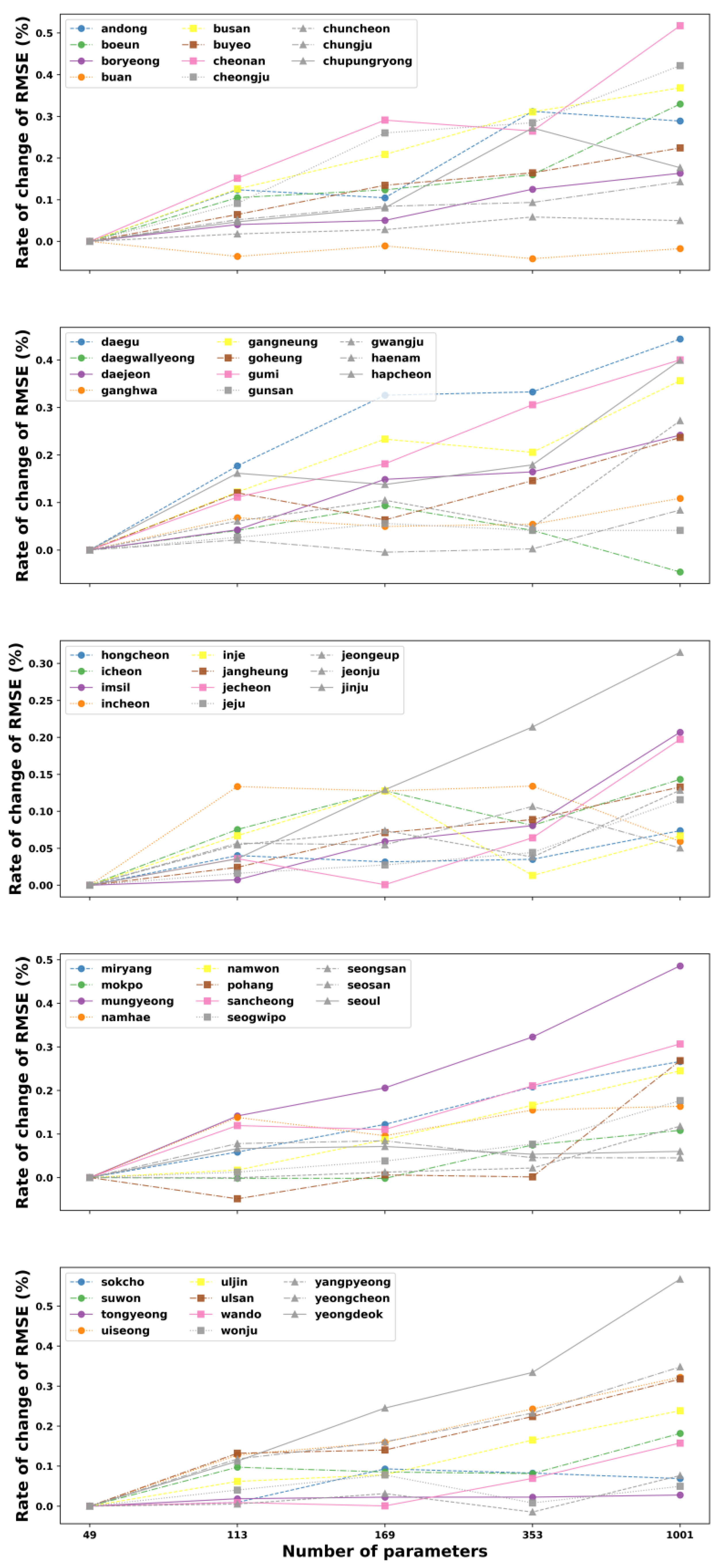Thus, as the results are depicted in Figure 3, Figure 4 and Figure 5, the proposed ANN with 49 parameters consistently outperforms the other parameters at almost all stations in South Korea, since it produces the lowest change in error for different model configurations. Taking the single-hidden layer ANN as an example, the rate of change of the RMSE slightly increases with the extension of parameters for most sites (see Figure 3).

However, we can also observe that the increased parameter size of the ANN model made the error’s change decrease lightly at Buan stations. Moreover, several sites have the lowest change values of RMSE at the parameter of 1001, such as Daegwallyeong, Gunsan, Hongcheon, and Tongyeong. These sites have an increasing trend of error when the number of tunable parameters in the network is raised from 49 to 169 (Hongcheon) or 353 (Daegwallyeong, Gunsan, and Tongyeong) before declining to the lowest point at 1001. 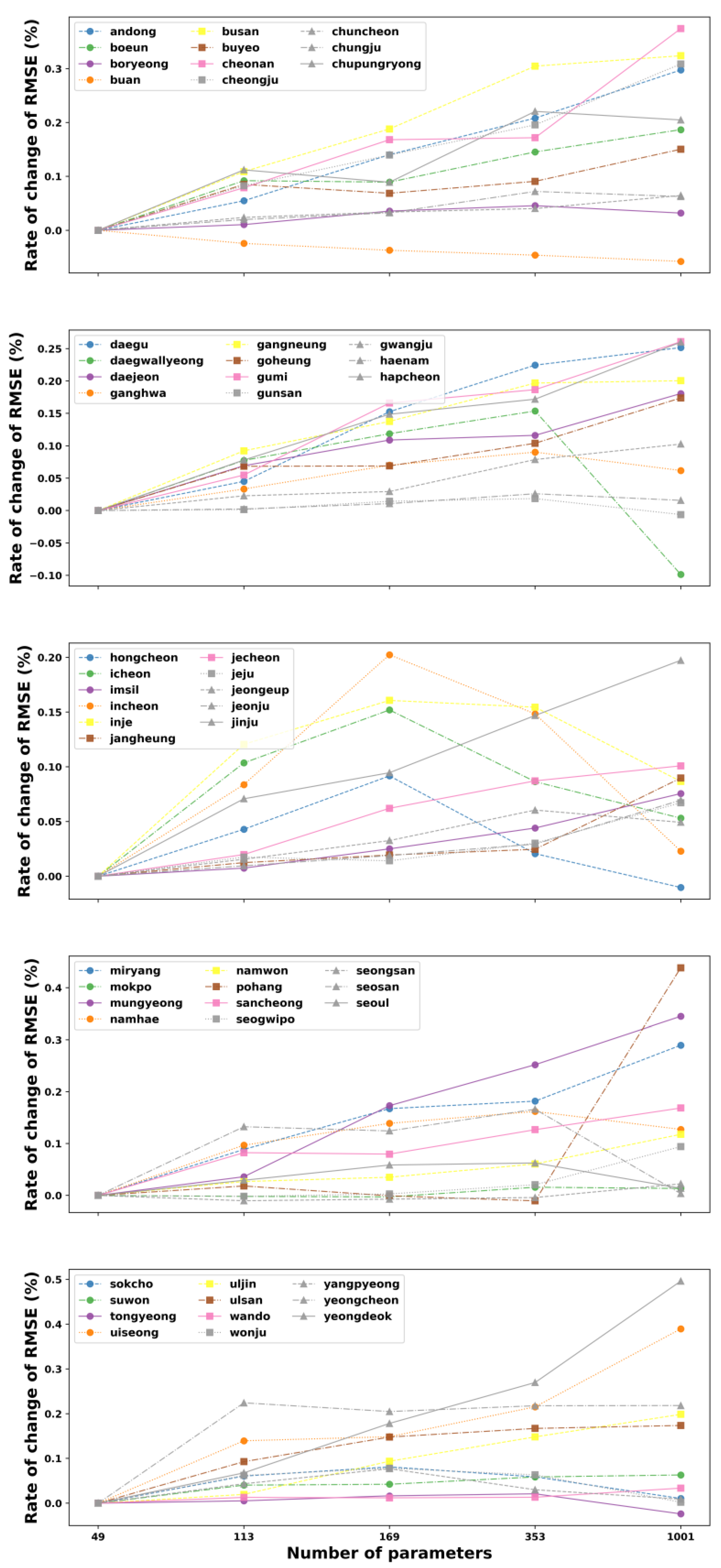Similarly, Figure 4 illustrates the general relationship between the total numbers of parameters versus the rate of change of RMSE on testing data in all 55 stations for three hidden layers. It can be noted from this figure that in the majority of stations, the rise of parameter numbers makes the performance of the model worse due to the increase in the change of RMSE. In contrast, few stations have the best results at the parameter of 133 (Pohang), 169 (Haenam), 353 (Buan and Yeongdeok), and 1001 (Daegwallyeong). Although the fluctuation of the RMSE’s change rate for the three-hidden layer ANN, corresponding to various parameter sizes, varies from site to site, the ANN model with a structure of 49 trainable parameters still shows the best solution for predicting the maximum temperature one day ahead for most stations in South Korea.

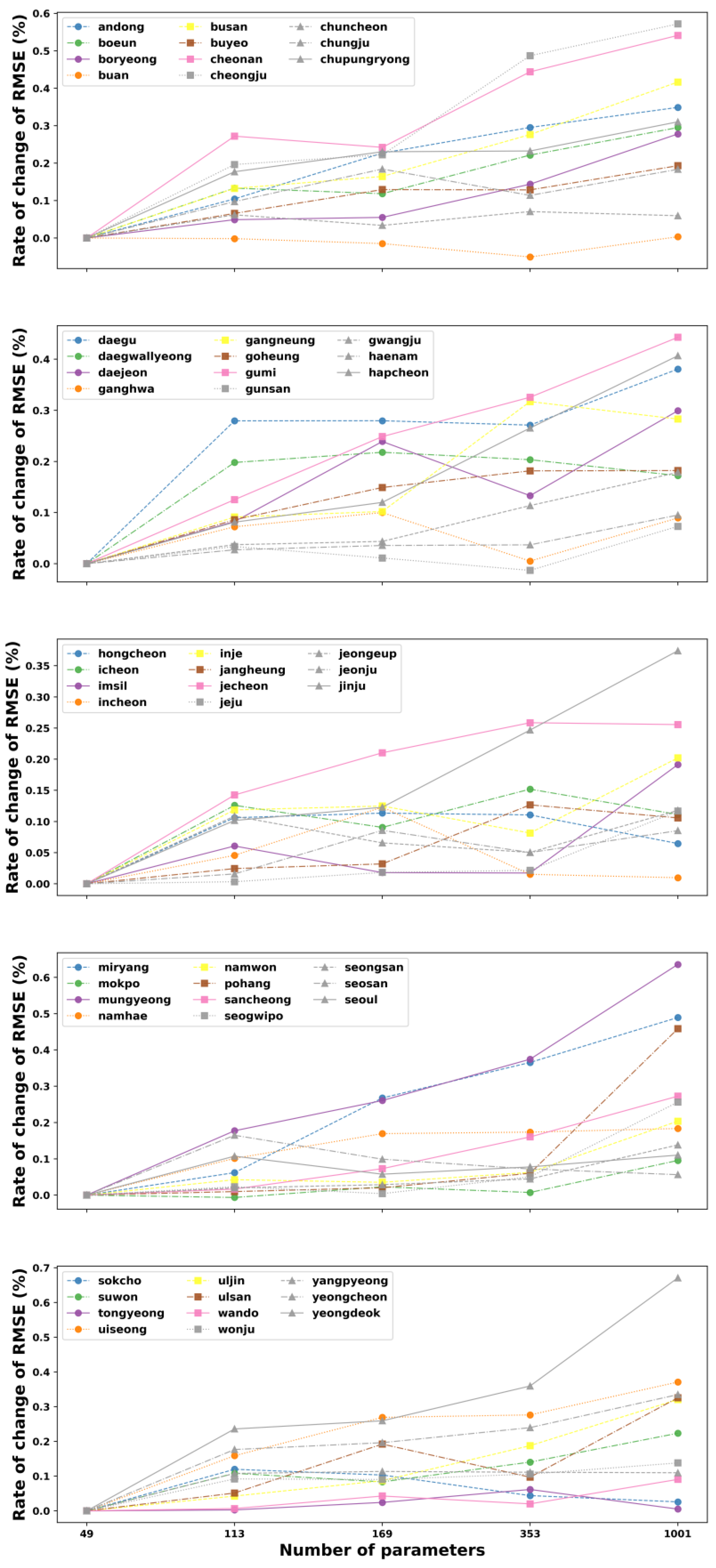
In the case of five hidden layers, it can be observed from Figure 5 that the 49-parameter ANN model continues showing the smallest error in 52 out of the total 55 stations. In most cases, the increase in the number of parameters deteriorates the performance of the ANN model. However, it should be noticed that the model achieves the best result at the parameter of 353 in Buan and Gunsan stations while the smallest RMSE in Mokpo is obtained at the parameter of 119.

Figures S1–S4 (see Supplementary Materials) depict the RMSE of the ANN models with three different hidden layers that vary the number of parameters from 49 to 1001. The learnable parameter is an important parameter that may affect the ANN’s performance for predicting the maximum temperature in the future. For a better assessment, the five-run average and standard deviation of the performances of each considered parameter and associated ANN architecture are depicted in those figures for each station separately. Generally, in most stations, there is a slight increasing trend of the RMSE when the number of parameters is increased. Furthermore, it can be seen from those figures that the ANN with parameters at 49 outperformed the parameters of other models, since it produced the lowest RMSE compared to others, except for Buan, Daegwallyeong (Figure S1), and Tongyeong stations (Figure S4), while the models having 1001 parameters yielded the worst results at around 50% of total stations, in comparison to other numbers of parameters. The difference in performance when the number of parameters increased from 49 to 1001 was marginal, but the value of 49 still leads to slightly better results. Thus, it can be noticed from these results that the testing RMSE of lower parameters is maybe better than higher parameters considering the low amount of neurons, and the models with 49 parameters are sufficient to forecast the maximum temperature variable. Nevertheless, there is an adaptive amount of parameters in the model in terms of hidden layers in some cases. For example, at Tongyeong stations (Figure S4), the model having one hidden layer showed the smallest RMSE at the parameters of 1001, while three and five-hidden layer models produced the best results with 49 parameters. In another case, 49 was the best number parameters for one and five hidden layers; meanwhile, three hidden layers presented the best performance at 353 parameters at Yangpyeong station (Figure S4). Besides, it is worth noting that at the same parameter number, the values of the RMSE for the one-, three-, and five-hidden layer models were comparable in most of the stations. However, the significant differences among the three configurations of the model can be observed at the 1001 parameters such as Boryeong, Cheongju, Daewallyeong (Figure S1), Mokpo (Figure S3), Wonju, and Yangpyeong stations (Figure S4) or the 353 parameters such as Ganghwa (Figure S1), Incheon, Jangheung (Figure S2), Seosan (Figure S3), and Yangpyeong stations (Figure S4). In addition, the RMSE shows little sensitivity to changes in the number of hidden layers in some stations, especially at high parameters due to the large fluctuation of standard deviation values. For example, in Tongyeong station (Figure S4), at the same parameter number of 353 or 1001, the standard deviation values of the RMSE of three- and five-hidden layer models are considerably larger than that of the one-hidden layer model. The trend is more evident for predicting the maximum temperature as the total number of parameters increased and occured in some stations, such as Buan, Daegwallyeong, Chuncheon (Figure S1), Wonju, or Yangpyeong stations (Figure S4). It can be suspected that the performance of the model may be significantly affected when the structure of the model becomes more complex. Based on the variation model performance in terms of hidden layers and parameters, it can be concluded that both the number of parameters and hidden layers were important to the model’s performance, and the selection of parameters and hidden layers needs considerable attention because of the fluctuation in error.

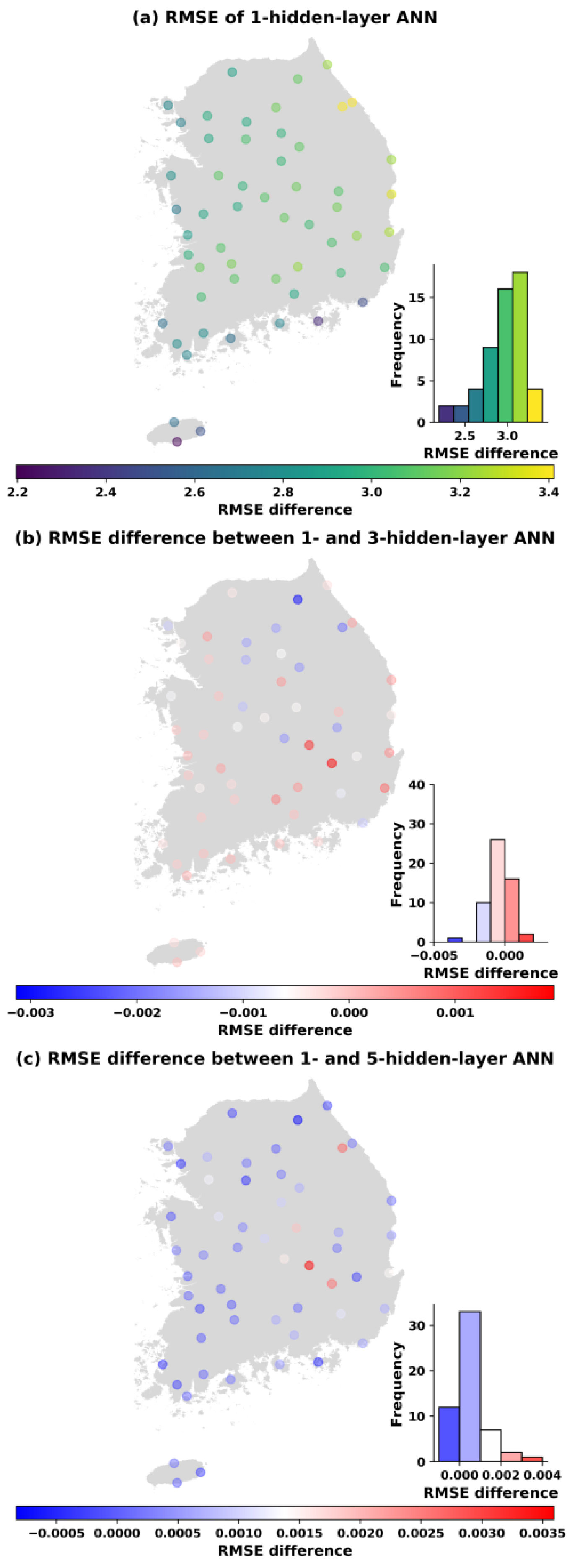
3.2. Effect of the Number of Hidden Layers

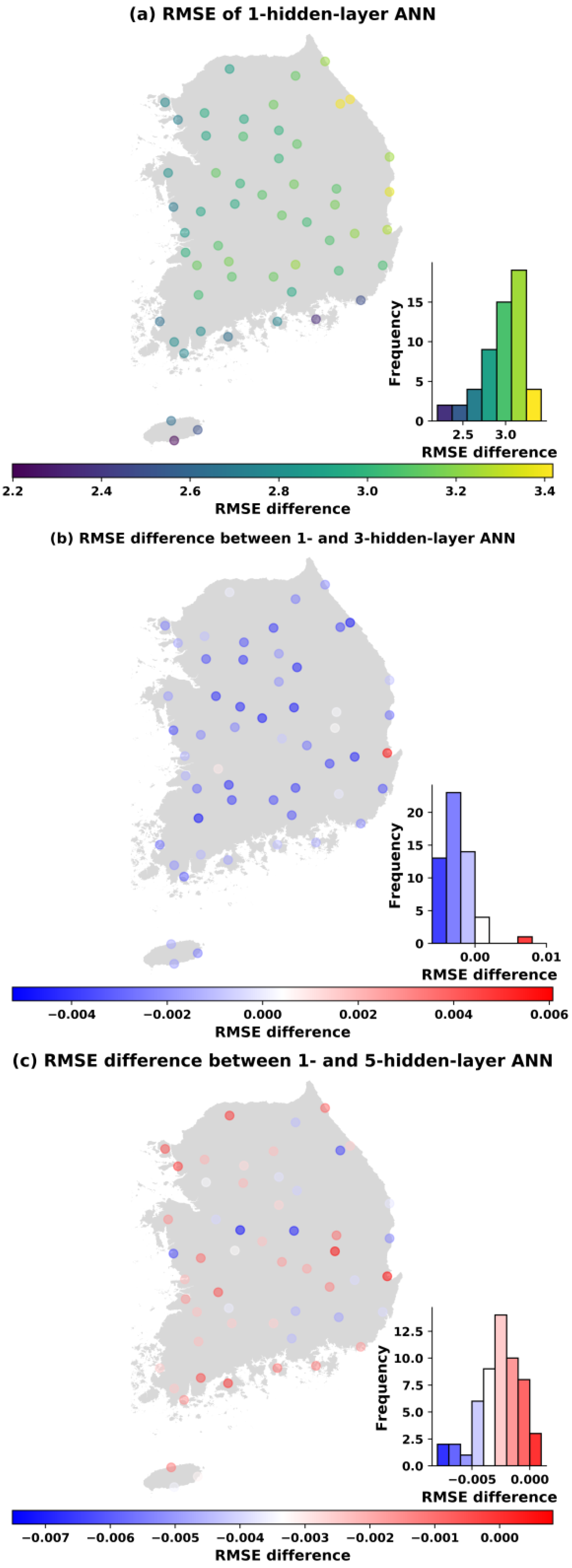
Figure 6, Figure 7, Figure 8, Figure 9 and Figure 10 show the spatial distribution of the ANN performances in the test period. Accordingly, a significant decrease in error is likely to move from the eastern to the western and southern part of South Korea with 49 learnable parameters (see Figure 6).

Similar spatial distributions of the changes in RMSEs also occur in Figure 7, Figure 8, Figure 9 and Figure 10 when the number of parameters is increased to 113, 169, 353, and 1001. It can be concluded that the ANN models perform better in western and southern Korea (left panels). Moreover, the visualization of the differences in the RMSE between one hidden layer and three hidden layers (middle panels) as well as between one hidden layer and five hidden layers (bottom panels) at each station is also shown in Figure 6, Figure 7, Figure 8, Figure 9 and Figure 10. It is noticed that with the same number parameters of 49, while one-hidden layer model presented better results than the three-hidden layer model at over 60% of total stations, the five-hidden layer model performed slightly greater than the one-hidden layer model at around 79% of stations where RMSE differences greater than 0 were found (see Figure 6). However, with the increase in the number of parameters, the ANN models with one hidden layer produced better results than the three- and five-hidden layer models in almost all stations.

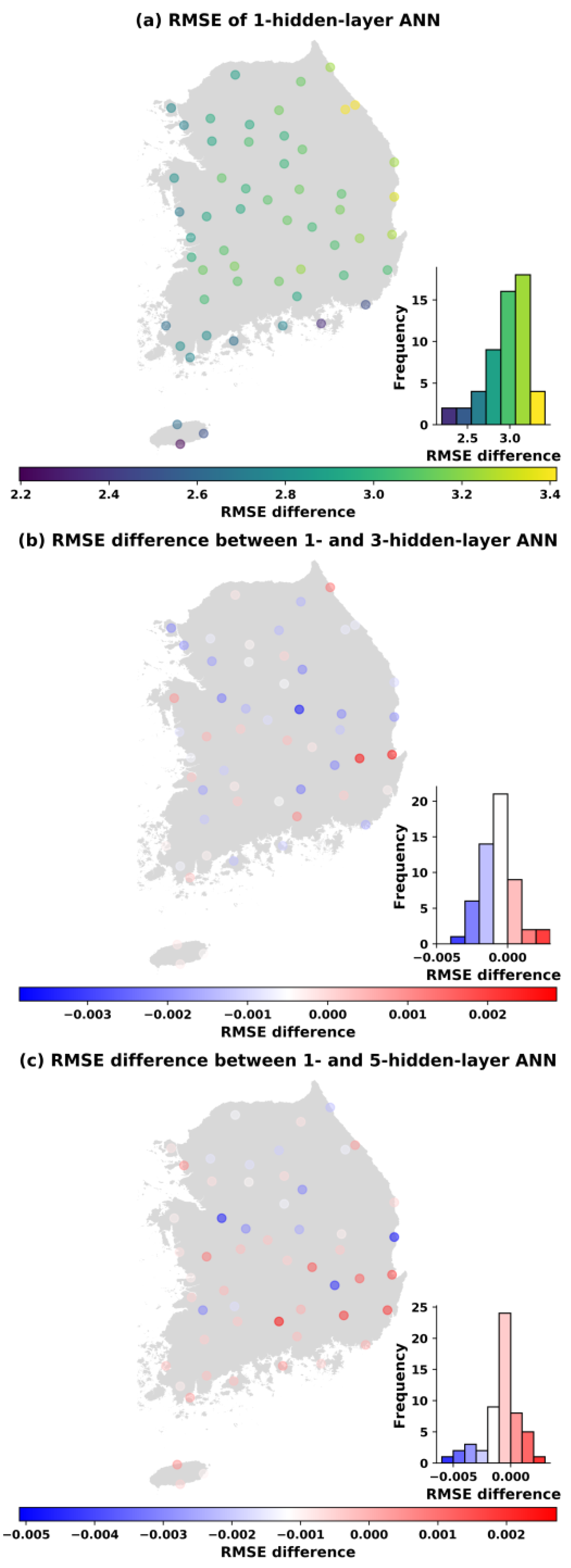
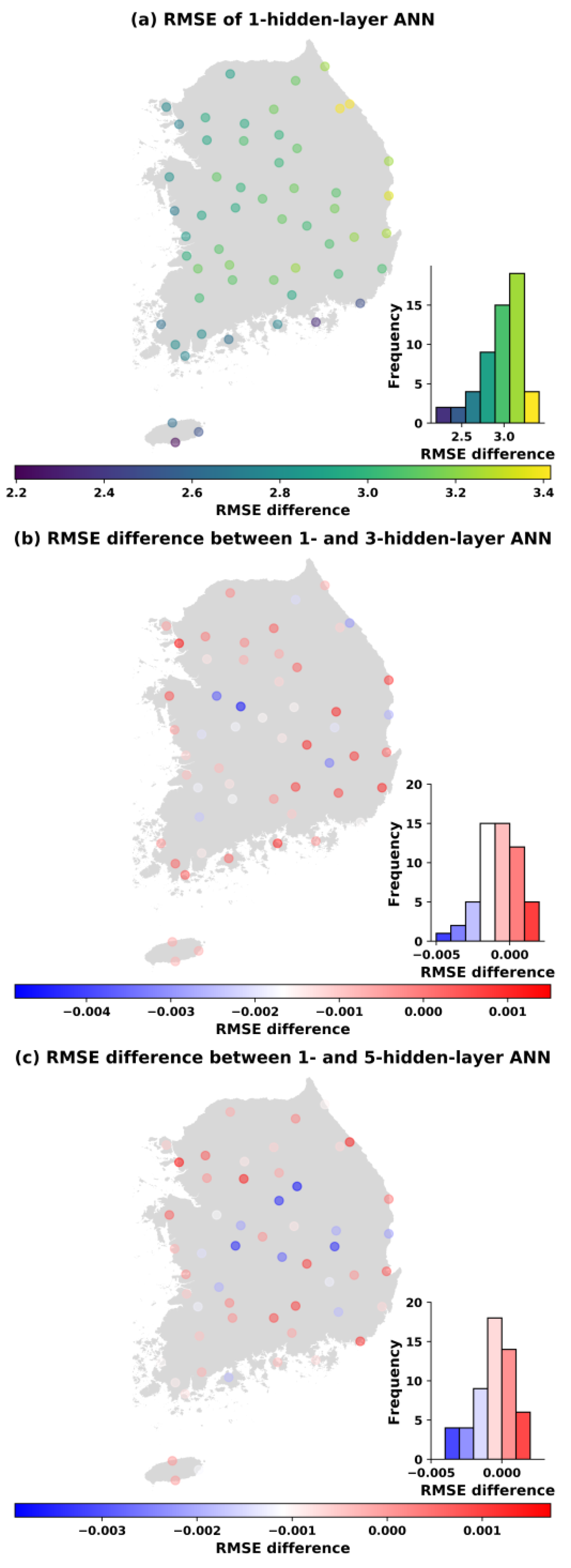
For example, Figure 7 indicates that, based on the RMSE of the testing sets, the one-hidden layer model achieves a better performances at 42 and 41 stations, respectively, when the number of parameters is 113, compared to the three- and five-hidden layer models. Similarly, at the parameter number of 169, and from the histogram of RMSE differences (Figure 8), we can see that the one-hidden layer structure generally obtained a smaller error than three and five hidden layers for most sites. However, it was noted that the multi-hidden layer models improved the performance of temperature prediction at some stations (17 stations with three hidden layers and 20 stations with five hidden layers) in comparison to one hidden layer. 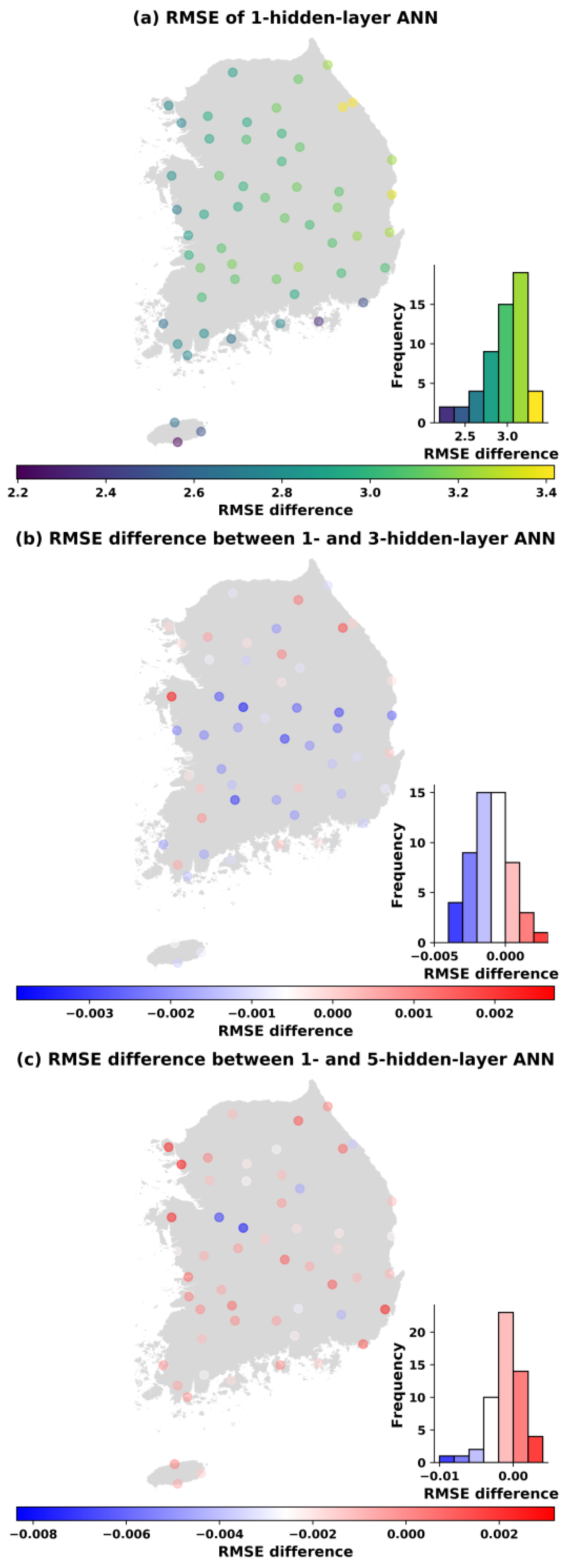Moreover, the number of sites that obtained a smaller RMSE with multiple hidden layers decreased slightly when the number of parameters was increased to 353 (Figure 9). Out of 55 stations, there were 12 stations with three hidden layers having smaller errors than one hidden layer, and 18 stations with five hidden layers had better performance than one hidden layer. Finally, Figure 10 compares the ANN models in the test case in the name of the RMSE and hidden layer with 1001 trainable parameters. As the results showed, the one-hidden layer ANN generated a better result at almost every station than the three and five hidden layers. The three- and five-hidden layer ANNs had higher RMSE than one hidden layer in five and three stations out of 55 stations, respectively. The results were worth emphasizing that the deep ANN with various parameters trained for all stations generated a certain number of basins with lower performance than a single-hidden layer network, but the stations where this occurred were not always the same.

4. Summary and Conclusions

In this study, different hidden layer ANN models with various interior parameters were employed to forecast 1 day maximum temperature series over South Korea. This study aimed to explore the relationship between the size of the ANN model and its predictive capability, revealing that for future predictions of the time series of maximum temperature. In summary, the major findings of the present study are as follows.

Firstly, a deep neural network with more parameters does not perform better than a small neural network with fewer layers and neurons. The structural complexity of the ANN model can be unnecessary for unraveling the maximum temperature process. Even though the differences between these models are mostly small, it might be useful to some applications that require a small network with a lower computational cost because increasing the number of parameters may slow down the training process without substantially improving the efficiency of the network. Importantly, it can be observed that a simple network can perform better than a complex one, as also concluded in other comparisons. The authors in Lee et al. [20] showed that a large number of hidden neurons did not always lead to better performance. Similarly, in our previous study, the hybrid method of ANN and the genetic algorithm was applied to forecast multi-day ahead maximum temperature. The results demonstrated that the neural network with one hidden layer presented a better performance than the two and three hidden layers [14]. Nevertheless, too many or lesser amounts of parameters in the model can make the RMSE of the model increase, such as in the Buan station. This could be explained by an insufficient number of parameters causing difficulties in the learning data, whereas an excessive number of parameters might lead to unnecessary training time, and there is a possibility of over-fitting the training data set [21].

Secondly, although the performances of the models corresponding to different hidden layers are comparable when the number of parameters is the same, it is worth highlighting that five-hidden layer ANNs showed relatively better results compared to one and three hidden layers in the case of 49 parameters. However, when the number of parameters was large, the model with one hidden layer obtained the best solutions for forecasting problems in most stations.

Finally, the model’s parameters and the degree of effectiveness of the hidden layers are relatively competitive in forecasting the maximum temperature time series due to variations in errors. Additionally, when the number of parameters is large, the significant difference of model outputs from various hidden layers can be achieved.

As future work, we are interested in investigating the effect of more parameters such as the learning rate or momentum on the system’s performance. Moreover, conducting an intensive investigation on the effect of parameters on other deep learning approaches for weather forecasting, such as a recurrent neural network (RNN), long short-term memory (LSTM), and convolutional neural network (CNN) is a matter of interest for our future research. Besides, the sensitivity analysis or critical dependence of one parameter on others may be involved for further research.