Article

PM10 and PM2.5 Qualitative Source Apportionment Using Selective Wind Direction Sampling in a Port-Industrial Area in Civitavecchia, Italy

by
Maria Eleonora Soggiu
1,
Marco Inglessis
1,
Roberta Valentina Gagliardi
1,
Gaetano Settimo
1,
Giovanni Marsili
2,
Ivan Notardonato
3 and
Pasquale Avino
3,*
1
Italian Institute of Health, Viale Regina Elena 299,I-00185 Rome, Italy
2
Consorzio per la Gestione dell’Osservatorio Ambientale, Via delle Saline 18, Tarquinia, I-01100 Viterbo, Italy
3
Department of Agriculture, Environmental and Food Sciences, University of Molise, via F. De Sanctis, I-86100 Campobasso, Italy
*
Author to whom correspondence should be addressed.
Atmosphere 2020, 11(1), 94; https://doi.org/10.3390/atmos11010094
Submission received: 30 November 2019 / Revised: 6 January 2020 / Accepted: 7 January 2020 / Published: 13 January 2020
(This article belongs to the Special Issue Exposure Assessment of Air Pollution)

Abstract

:
The possibility to discriminate between different emission sources and between natural and anthropogenic contributions is a key issue for planning efficient air pollution reduction and mitigation strategies. Moreover, the knowledge of the particulate matter (PM) chemical composition for the different size fractions is recognized as increasingly important, in particular with respect to health effects of exposed population. This study is focused on the characterization of PM10 and PM2.5 main sources located in the Civitavecchia harbor-industrial area (Central Italy), namely a large coal-fired power plant, a natural gas power plant, the harbor area, the vehicular traffic (due to both the local traffic and the highway crossing the area) and small industrial activities. The approach was based on PM10/PM2.5 samples monthly collected for one year and a further relative chemical characterization of organic and inorganic fractions. Wind-select sensors, allowing a selective PM10 and PM2.5 sampling downwind to specific emission sources, were used for the overall sampling. This methodology manages to explain specific emission patterns and to assess the concentration levels of the micro pollutants emitted by local sources and particularly toxic for health. A descriptive statistical analysis of data was performed, also verifying the occurrence of legislative threshold exceedances. Moreover, in order to highlight the contribution of specific sources, the differences in the measured micro pollutants concentrations between wind directions, PM size fractions and sampling sites have been investigated, as well as the seasonal trends of pollutants concentrations. These results allow to highlight that the applied methodology represents a valid support in source apportionment studies.

1. Introduction

With the progressive reduction of emissions from large combustion plants, from road traffic, the emissions from other sources, as non-road mobile sources, are becoming increasingly important, in particular in port areas where intense commercial activities are present. Many cities in Europe and even in Italy have great difficulties in compliance with the limits imposed by European Union legislation on air quality. The presence of harbors/ports in urban areas should be considered as an important pollution source, often also with the presence of cruise terminals, which are completely integrated into the cities. Furthermore, the International Maritime Organization (IMO) has estimated that more than 90% of world trade is moved by sea as the maritime transport is the cheapest way to move goods and raw materials [1].
In large harbors, air quality is measured by monitoring the atmospheric concentrations of the pollutants regulated by Legislative Decree 155/10 [2], such as nitrogen dioxide (NO2), sulfur dioxide (SO2), carbon monoxide (CO), ozone (O3), benzene (C6H6), PM10 and PM2.5 through mobile and fixed monitoring stations.
Among the most polluting factors, besides land-based port activities, the main ship emissions are nitrogen oxides (NOx), sulfur oxides (SOx), CO, particulate matter (PM) and hydrocarbon (HC) due to the engine combustion [3,4,5,6]. Ship emissions account for respectively 2.7%, 15% and 4–9% of the global anthropogenic CO2, NOx and SO2 emissions [7], whereas PM10 and PM2.5 levels are related to primary emissions from fuel oil combustion but also to the formation of secondary aerosols [8]. These pollutants are the main chemicals involved in processes leading to acidification and eutrophication as well as formation of ground level ozone [9]. The pollution of port cities is mainly due to the stationing of cruise ships moored to the piers [10]—these floating cities must keep the engines running both to work and to provide on-board passenger services [11]. By this way, highly toxic fumes are emitted into the atmosphere compromising the air quality [12], the environment [13] and, consequently, the public health [14,15]. Based on previous evidences [16,17,18], it can be hypothesized a specific role of environmental pollution of industrial origin on the current frequency of lung cancer in Civitavecchia. Infant respiratory disease is strongly influenced by environmental exposures. Recent studies conducted in Europe and the United States have highlighted a role of air pollution in the aggravation of bronchial asthma, a pathology particularly frequent in pediatric age [19,20,21] As a consequence, in complex areas where multiple sources are located, the study of contribution to PM emission from different sources is an important task in air quality management. These studies are performed using the source apportionment methodologies [22,23,24,25]. The possibility to discriminate among different emission sources and between natural and anthropogenic contribution is a key issue for planning efficient air pollution reduction and mitigation strategies, as pointed out by different authors [26,27,28]. Moreover, the knowledge of the chemical composition [29,30] for the different PM size is recognized as increasingly important, in particular with respect to the health effects of the exposed population [31]. All the considerations will be based on data obtained from wind-oriented samplings. This particular strategy, still considered rare, was introduced by Alleman et al. [32]. Each sampler, coupled with a wind sensor allowing the turning on and off of the instrument depending on wind direction and speed, alternately collects PM coming from the wind directions—in this way, each airborne sample, related to different wind conditions, is not predominantly associated with a direction but is exclusively connected with a single direction [33,34,35]. Figure 1 shows the sampler used in this study.
The aim of this study is the identification of main emitting sources of PM10 and PM2.5 in the Civitavecchia port-industrial area (Central Italy), namely a large coal-fired power plant, a natural gas power plant, the harbor activities, the vehicular traffic (due to urban traffic and to the highway crossing the area) and small industrial companies located in the town. Our study also provides precious information on the chemical composition of the PM10 and PM2.5 collected, effective to explain specific sources emission patterns as well as to assess the concentration levels of micro pollutants (MPs), particularly toxic for human health.

2. Experiments

Characterizazion of the Sampling Site

The investigated area (Figure 2) is affected by the presence of different anthropogenic sources. Civitavecchia is a city of about 53,000 inhabitants, hosting a commercial port which moves about 4 million people and 11 million tons of goods per year. In recent years, it has become a leading port for cruise ships in the Mediterranean Sea. Furthermore, Civitavecchia is the third Italian energy hub, with a coal-fired power plant (Torrevaldaliga North) of 1980 MW and gas turbine plant (Torrevaldaliga South) of a 1200 MW. This area is crossed by an important highway (Rome-Tarquinia) and the Aurelia state road is affected by freight traffic.
With the aim to study the sources contribution to PM environmental concentrations, the chosen sampling method is represented by a PM sampler coupled with a wind-select sensor that allows collecting PM on different cartridges according to specific wind directions (WindSelect+, MonitoringSystems GmbH, Austria). In fact, this device allows to set two user-defined wind direction sectors, corresponding to specific emission sources (i.e., coal-fired power plant, sector #1 and harbor, sector #2). By this way, the wind sensor activates the different cartridge and acquires the air volumes when the wind comes from these wind sectors; a third sector (sector #3) is activated when the wind blows from all other directions.
In this study, two sampling sites have been identified in the area—the first inside the densely populated urban area of Civitavecchia, downtown Civitavecchia (U), was placed on the roof of a public building at about 25 m above the ground level, the second one was located just outside the urban area, in an Urban Background (UB) site, at 3 m above the ground level. The U and UB sites, both equipped with a PM10 and PM2.5 wind-select sampling device, are 12 km apart. The samplers have been configured to collect airflows downwind the coal-fired power plant (sector #1) and downwind the port area (sector #2), whereas all other wind directions correspond to sector #3. For the U site the sectors were—sector #1: 300°–330°, downwind the coal-fired power plant direction; sector #2: 200°–280°, downwind harbor; sector #3: all other directions. For the UB site the three sectors were: sector #1: 270°–300°, downwind coal-fired power plant direction; sector #2: 210°–260°, downwind harbor; sector #3: all other directions.
The study was carried out from July 2015 to June 2016. PM10 and PM2.5 samplings were performed by means of wind-selective samplers; the duration of each sampling was approximately 30 days. On the PM10 and PM2.5 samples monthly collected, chemical analyses were performed for determining the concentrations of organic and inorganic species in both aerosol size filters, focusing on those related to coal combustion, as heavy metals (i.e., As, Cd, Mn, Ni, Pb, Se, V, etc.), Polycyclic Aromatic Hydrocarbons (PAHs), Polychlorinated Biphenyl (PCBs), Polychlorodibenzodioxins and Polychlorodibenzofurans (PCDD/Fs) [36,37,38,39,40,41]. For the depositions, the measurements were carried out with bulk samplers according to UNI EN 15841:2010 and UNI EN 15980:2011 standards. The detection system consists of glass fiber filters and adsorbent cartridges (Polyurethane Foam, PUF, and Amberlite XAD-2). For the organic compounds the samples were extracted by Accelerated Solvent Extraction (ASE) and the analyses were carried out by HRGC-HRMS (High Resolution Mass Spectrometry; R > 10,000), according to the indications of UNI EN 1948:2006 parts 2 and 3, for the determination of PCCD/Fs and PCBs and according to the indications of ISO 122,844 and UNI EN 15549:2008 (specifically for benzo (a)pyrene) for determining PAHs whereas the determination of the inorganic fraction, that is, metals, was performed by IPC-MS, according to UNI EN 14907:2005, after that the samples were mineralized in HNO3 according to the UNI EN 14902:2005. Finally, a particular attention was devoted to investigating the Limit of Detections (LODs) of each compound; they can be resumed as follows—metals 0.1 ng; PAHs 10 ng; PCDD/Fs 100 fg; PCB 1000 fg.

3. Results and Discussion

An analysis on the meteorological conditions of the area and on operating characteristics of the coal-fired power plant was initially performed.

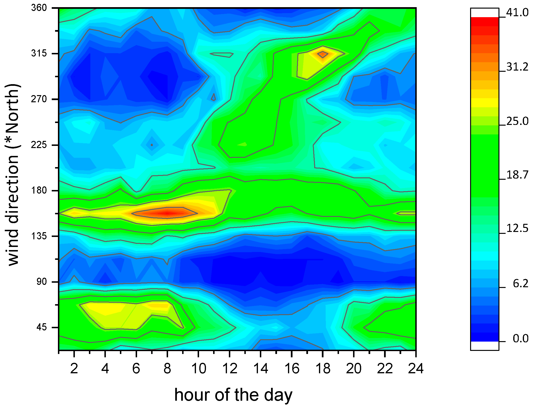
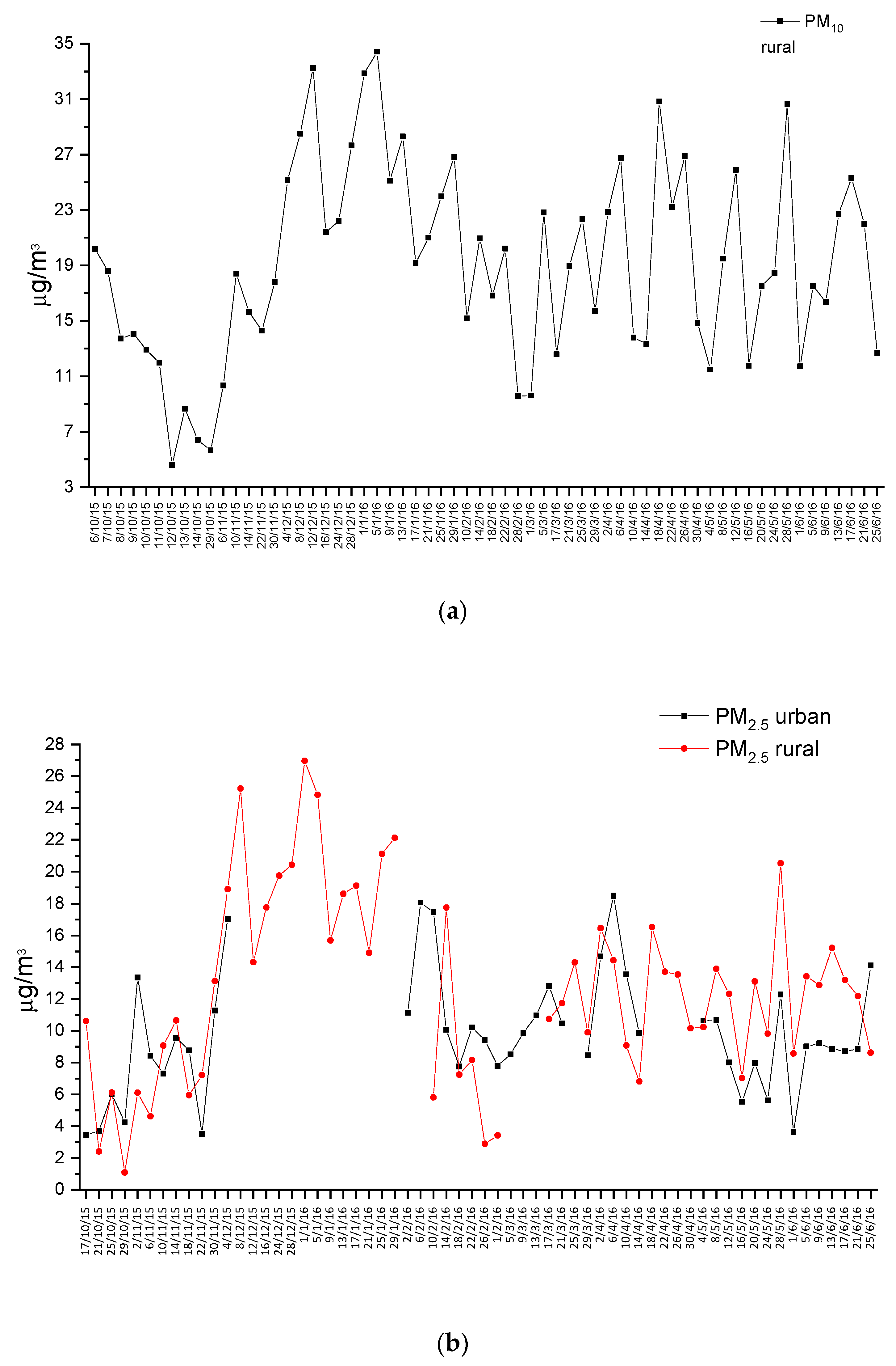
3.1. Meteorological Conditions

The analysis of the meteorological conditions was carried out on data acquired from the meteo-station located inside the coal-fired power plant settlement at high altitude (120 m).
The available data cover the period between June 2015 to March 2016. The analysis of wind directions showed the expected seasonal variability during all the study period. In general, the winds from East have low frequencies, in some periods they are absent. The most frequent directions are those associated with the sector from South-West to North-West, the winds from the South are predominant in the months of October and February, whereas the North-East sector is present with higher frequencies in the months of September, October, November and March.
Figure 3 shows how the wind directions change during the daily hours, as measured in the period June 2015-March 2016. Until mid-morning hours the North-East and South-East directions are prevalent, therefore the wind turns and during the afternoon West and North-West sectors are the predominant wind directions, in particular the North North-West sector during the evening (hours 16–19). Even the wind speeds show a variability strictly related to wind direction. On average, higher speeds are associated with winds from the North-East and South-East directions. A frequency analysis of the daily hours in which the wind sectors are active was also performed. Sector #1 of the U site is downwind more frequently during the evening hours, the other sectors, that is, sector # 2 of U site and sectors # 1 and # 2 of UB site, are downwind more frequently during the mid-day hours and early afternoon.

3.2. Coal-Fired Power Plant Information

The analysis of operation characteristics of the coal power plant was performed, taking into account data from the Continuous Monitoring System installed on the three stacks (Table 1). Total Suspended Matter (TSM) emission data (in mg Nm−3) from the period June 2015 to March 2016 were analyzed.

3.3. Chemical Analysis and Relative Source Apportionment

As said before, the study was addressed for identifying the sources (source apportionment) of organic and inorganic contaminants in similar complex areas, using the wind-select monitoring devices. This approach allows to highlight the relationships between the presence/abundances of specific chemicals and the wind/sampling directions. Further, before starting with the results, it should be underlined that the domestic heating, another well-known source potentially affecting the urban air quality, in Civitavecchia is characterized by methane gas—in this case the authors considered its contribution to be superfluous, also considering the average temperatures ranging between 13.5–21.1 °C during winter/autumn period and 17.3–25.9 °C during spring/summer period, with a yearly average of 19.5 °C, 66 rainy days and Relative Humidity (RH) 74.7% (source—Stazione Meteorologica di Civitavecchia).
At the same time, concentrations data of PM10 at the suburban site and PM2.5 in the two sites, urban and suburban locations, were acquired for all the period. These data were measured by gravimetric method with instrument located close to the wind-select samplers. Figure 4 shows the gravimetric measurements performed in urban and suburban area—particularly, Figure 4a shows the PM10 behavior for the entire period whereas Figure 4b PM2.5 in both locations.
In the urban area, due to maintenance works, data of PM2.5 are missing between December and January, (in Figure 4b there is a “hole” in that period). The concentrations are similar on both sites—at the suburban site, an average value of 12.6 µg m−3 is recorded whereas at urban site a mean value of 9.7 µg m−3. This is most likely due to the missing measurement period (December–January) at this location—in fact, wintertime shows unfavorable meteorological conditions for the pollution dispersion [42,43], allowing high levels of pollutants. PM10 measurements at the suburban site show a mean value of 19 µg m−3 for the entire period—the measurements confirm the high pollution level recorded during January and December period as provided by the Figure 4a.
The results of chemical analysis performed on PM2.5 and PM10 are represented in Table 2 and Table 3 for the mean levels of inorganic (i.e., metals) and organic (PCDD/Fs, PAHs and PCB and DL-PCB) substances in cartridges sampled for each sector. Data in Table 2 and Table 3 concern the whole period mean concentration of each pollutants both in urban and suburban site. In Tables S1–S8 of the Supplementary Material report all the analytical determinations performed sector-by-sector during the whole sampling periods in both locations are reported.

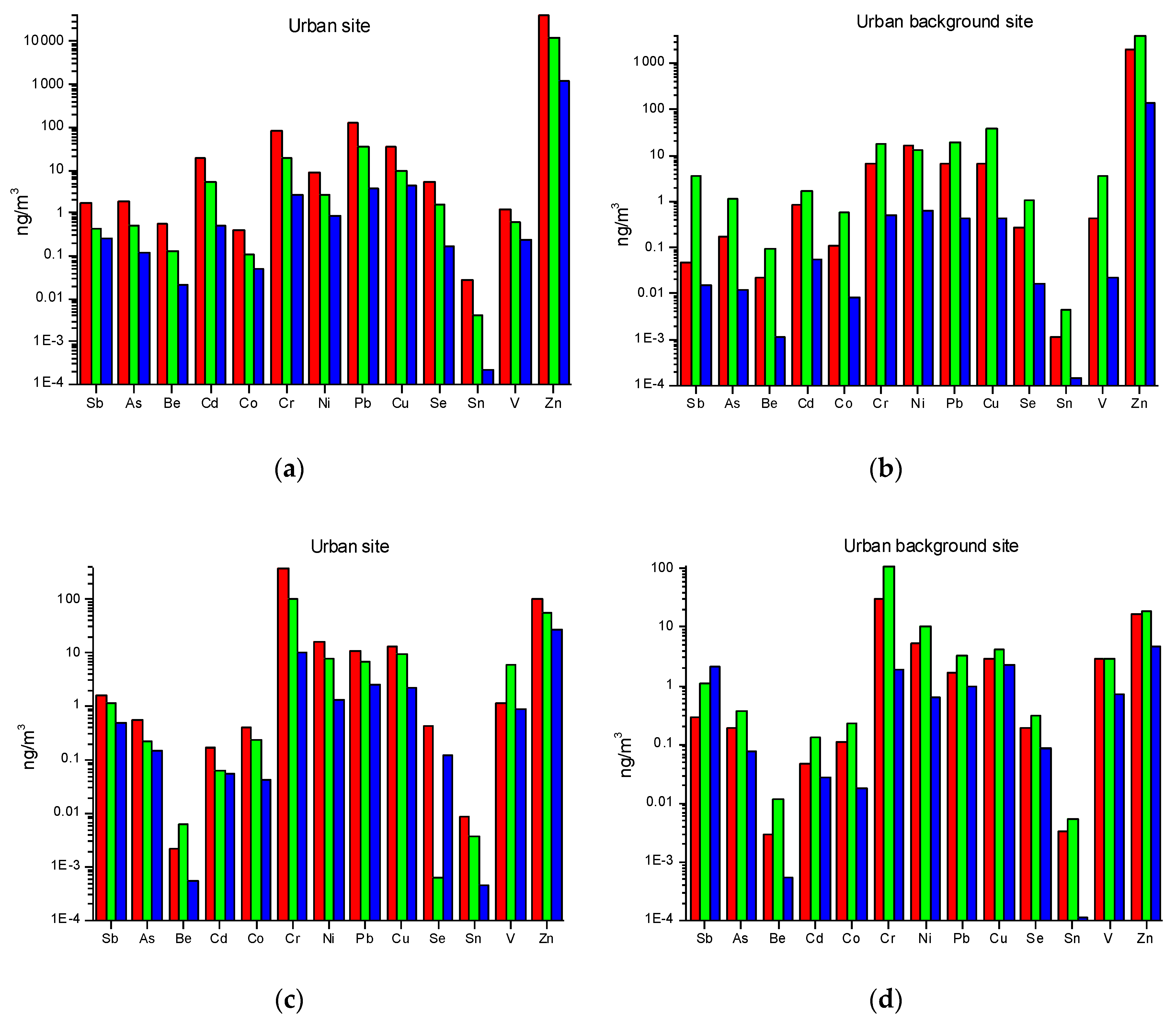
3.3.1. Inorganic Fraction

The study of inorganic substances has been addressed for elements potentially representative of anthropic sources with high interest for public health. With this aim, in addition to the metals routinely monitored in compliance with the air quality law (Legislative Decree 155/2010), that is, As, Cd, Ni and Pb, the chemical analysis also concerned Sb, Ba, Be Co, Cr, Mn, Cu, Se, Sr, Tl, Te, Ti, V and Zn. These elements are generally present with different abundances and in different oxidation states in the PM size fractions.
The analytical determinations of metals for each monitoring site and both PM fractions and sectors, are showed in Tables S1 and S2 of the Supplemental Material for the U and UB sites, respectively. Figure 5a,c for U site and Figure 5b,d for UB site, respectively, report all the concentrations measured during the entire sampling period.
For a comparison of concentration values measured regulated metals (As, Cd, Ni and Pb) with limit established by regulation, it must be taken into account the different sampling methods used with those defined by law. For the regulated metals, it is possible a comparison only for determinations on the PM10 fraction, even though the integration time of PM10 in this study is on monthly average and not daily as required.
Taking into account this caution, the following values deserve to be mentioned:
For the U site, sector #1, Cd 18.6 ng m−3 in autumn, As 6.67 ng m−3 and Ni 62.3 ng m−3 in spring period and 58.7 ng m−3 in summertime;
For the UB site, sector #2, As 9.86 ng m−3 in autumn and Ni 35.0 ng m−3 in summertime.
For other metals, in both stations, there is a higher percentage presence of Ba, Cr and Zn compared to the other metals. Further, in both stations, Cr shows peak concentrations mainly in the PM2.5 fraction, whereas Ba and Zn have the highest concentrations in the PM10 fraction. The different distribution of heavy metals in the two fractions, sometimes higher concentrations in the fine fraction than in PM10, is strange but not surprisingly. Such occurrence was found in other studies, also by some co-authors in samples collected downtown [44] or in industrial area [45].
The wind-selective analysis aims to highlight the pollutant origin, as the study main objective. On this regard, the inorganic fraction in PM10 and PM2.5 shows the following:
For U station the highest metal concentration values are recorded in sector #1, downwind the coal-fired power plant, both in the PM10 and in the PM2.5 fraction;
For the UB station the highest levels are, on average, recorded at sector #2, downwind the port area, both in the PM10 fraction and in the PM2.5 fraction.
Except for As, Ba, Se, Te and Zn, the higher concentration values for each element are observed at the U station. Some exceptions for specific chemicals are noted, mainly in the sector #2—Cr and Co in the PM2.5 fraction in winter and Ba, Sr and Zn in the PM10 fraction in summer. For the UB location, Zn in the PM10 fraction in the summer period when sector #3 is prevailing, Cu in the PM2.5 fraction in the autumn period during sector #1 prevailing and Ni in the PM10 fraction in the autumn period with high frequency of sector #1.

3.3.2. Organic Fraction

For organic pollutants, the concentration profiles of PAHs, PCCD/Fs and PCBs in the PM10 and PM2.5 fractions were studied.
In general the urban location measures higher PAH concentrations than the suburban one, even though the concentrations always remain below values compatible with the monitored urban territorial context, and, the benzo (a)pyrene (B (a)P) concentrations, that is, the only PAH regulated by Legislative Decree 155/2010 [1], in PM10 are always lower than 1.0 ng m−3 which is the limit for the annual average. Just one measure (Tables S3 and S4 of the Supplementary Material), performed in U site records a concentration of B(a)P greater than 1.0 ng m−3.
Comparing the PAHs concentrations measured in the different sectors (Figure 6), sector #1 of the U location averagely records higher values than those observed in sectors #2 and #3, whereas in the UB area sector #2 records higher concentrations than those in sectors #1 and #3. Sectors #3 of both stations record the lowest PAHs concentrations.
Comparing the measures performed, it is noted that each PAH is concentrated in the PM2.5 fraction in all samplings carried out during the entire research study, except for measures performed at U area sector #1 during springtime, when some PAHs are below the LODs in PM2.5 fraction whereas they are observed in PM10 samples. For the UB location the measures always show higher concentrations in PM2.5; only once they are higher in PM10 for benzo(a)anthracene, B(a)P and benzo (b)fluoranthene, during the winter period.
The PAHs profile, representing the percentage of the concentration of each PAHs measured with respect the whole PAH concentration, can suggest some information on pollutants origin. Figure 7 shows the profiles of the mean PAHs levels for both the urban site during the winter period for each sector and particle size. Each profile is represented starting from the top to the bottom with the lightest PAH (2 benzene rings) to the heaviest (5–6 benzene rings). In U and UB site and in all sectors, naphthalene shows the highest concentration among the PAHs pollutants.
In general, all the measurements show the greatest contribution of the light PAHs (2–3 rings), present not more than 2% in the various samples, compared to the heavier ones. Besides to naphthalene, PAHs are phenanthrene, fluoranthene, anthracene, acenaphthene, chrysene and pyrene are the more abundant pollutants. Among the heavier PAHs, benzo[g,h,i]perylene and indeno[1,2,3-cd]pyrene show concentrations above the LODs. Generally, these two pollutants are related to diesel vehicular emissions [46,47,48,49,50,51,52] whereas the petrol vehicle emissions are characterized by B[a]P and dibenzo[ah]anthracene emissions [53,54,55,56,57]. For coal combustion, the PAHs profiles are generally characterized by a high presence of fluoranthene, pyrene, phenanthrene and anthracene, to which the chrysene and the isomer of benzo[k]fluorantene are added [58,59,60,61]. Regarding marine emissions, for ships at the port both in mooring and maneuvering, the PAHs fingerprint is represented by naphthalene, phenanthrene, pyrene, fluorene, followed by acenaphthylene and acenaphthalene [62,63,64,65].
The PAHs profiles observed in the two locations and for all the sectors show a predominant pyrogenic contribution, due to mixed contributions from the coal-fired power plant and from the port area. The high percentage of naphthalene, whose concentrations always remain comparable with those that normally occur in urban environments [66,67], would suggest a significant contribution from the emissions from the port area. Furthermore, the contribution of diffuse emissions arising from the port and the power plant, determines a PAH background contamination, especially for the lighter compounds (i.e., from naphthalene to chrysene). On this picture, under some circumstances, heavy vehicle diesel traffic adds its own contribution.
Like PAHs, the PCDD/Fs determinations (expressed as toxic equivalent, WHO-TE2005) in the two locations (Figure 8) show that sector #1 in U site records higher concentrations than those observed from the other two sectors, whereas for the UB location sector #2 records the highest concentrations compared to the other two.
Differently from PAHs, the lowest concentrations of PCDD/F not always are related to sector #3. In U site the sector #3 concentrations are similar and, on two cases, higher than those recorded by sector #2. This behavior is also evident in the UB location, where the sector #3 concentrations, particularly in PM2.5 fraction, reach high concentrations compared to those measured in the other sectors. The Figure 8 shows that the UB station sector #2 records in the winter and spring high concentrations, an order of magnitude higher than all the others. Similarly, to the PAHs, the PCDD/F concentrations (in equivalent toxicity WHO-TE) are generally higher in PM2.5 with respect to PM10, with the exceptions of spring-sector #1 U site and at spring-sector #2 of UB site. For the PCBs-DL (dioxin like) (Tables S7 and S8 of the Supplementary Material) comparable behaviors are highlighted in the two stations. In U site the higher concentrations are observed corresponding to sector #1, for the U site and to sector #2 for the UB area. In addition, pollutants concentrations are higher in the PM2.5 fraction compared to PM10. For PCBs-DL, the lowest concentrations are measured in relation to sector #3 for both stations, similarly to the PAHs behavior and differently from PCDD/Fs.
The Tables S5 and S6 of the Supplementary Material, respectively for U and UB sites, show the profiles of PCDD and PCDF congeners, for each sector, in PM10 and PM2.5 fractions. A first analysis shows that the congener concentrations are not always higher in PM2.5 than PM10. In fact, measures performed in autumn and spring for sector #1 in U site, show higher concentrations for some congeners in the PM10 fraction as well as at UB area for the sector #1 in winter. Also, in spring the three sectors in the UB site show higher concentrations for almost all congeners in the PM10 than in PM2.5.
Furthermore, all measures performed during the study and the profiles of the DL-PCBs are reported in the Supplementary Material. The results show that the congeners 118-PCB; 105-PCB and 156-PCB give the highest contribution in all sectors, fractions and locations.
The PCDD/Fs profiles for the spring sampling period in UB site are represented in Figure 9. These are always predominated by the presence of OCDD and OCDF. The profiles of sector #1 for the PM2.5 fraction, show a similar behavior during the different samplings periods with predominance of OCDD and OCDF, whose summed contribution varies between 60% and 93%, while the secondary contributions are of TCDF, HxCDF and HpCDF.
From the scientific literature [68,69,70,71,72] a similar profile is highlighted for PCDD/F emitted by large coal combustion plants. The PM10 and PM2.5 profiles at U sector #1 are similar.5 only in the autumn period, whereas they are different in the other two periods. The profiles of sector #2 of PM2.5 show greater variability, between periods and between congeners contributions. The PM10 profiles at sector #2 differ from those of PM2.5 and show differences among periods in terms of detected congeners and their relative contribution. The PCDD/Fs profile sampled at sector #3 in PM2.5 shows a wide variability of detected congeners in the different samples, according to the large sampling sector that cannot be associated with any specific source.

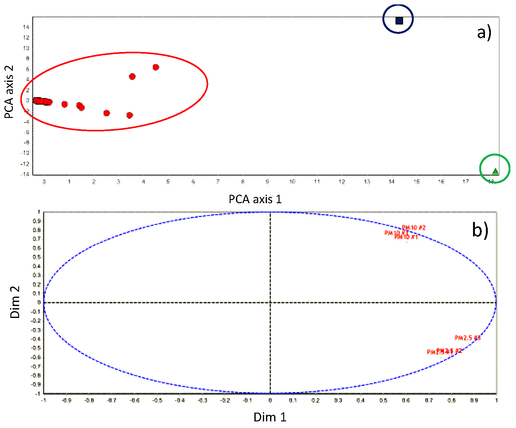
3.4. Chemometric Analysis

A statistical analysis has been carried out for overall the data. Preliminarily, a correlation among all the compounds has been investigated. In the U site the correlations between the PM fractions for the different sectors show a rather interesting trend. During autumn, high correlation coefficients (r) are observed between PM10 and PM2.5 for sectors #1 and #3 (0.952, 0.950) whereas it is lower at sector #2 (0.662). For the other periods, the PM10 and PM2.5 correlation coefficients are—in winter 0.878 sect #1, 0.975 sect #2, 0.882 sect #3; in summer 0.878 sect #1, 0.965 sect #2, 0.971 sect #3. The lower correlation coefficient in the autumn period between PM10 and PM2.5 in sector # 2 is probably due to a different weather condition, characterized by rapid changes of wind direction and speed, as expected in this season period. Different considerations can be drawn for the UB area—in the same period the correlation coefficient between PM10 and PM2.5 is good, 0.847 and in the other periods r in the three sectors is better (>0.810 during autumn, >0.924 during winter, >0.912 during summertime). Very good correlation coefficients (r > 0.970) are observed comparing similar fractions in same sectors, for example, r between PM10 in sector #1 urban area and PM10 sector #1 in suburban area is 0.977. It should be underlined that the sectors were chosen in order to show the same sources in that direction (i.e., sector #1 downwind coal-fired power plant; sector #2 downwind the port area; sector #3 other directions).
Further, the authors approached to study the correlation coefficients (r) among the different inorganic and organic compounds investigated. Table 4 shows the r determined during the entire campaign.
As it can be seen, for the inorganic fraction, that is, metals, the correlation coefficients between PM10 versus PM2.5 in the sectors #1 and #2 are poor whereas they improve over 0.6 in sector #3 of both sites. The low r in #1 and #2 shows different contributions affecting the metals levels over the coal-fired power plant (#1) or the port (#2); on the other hand, the good correlation coefficients found in #3 of both sites (sector #3: wind blows from all other directions) mean that the eventual metals emitted by these two anthropogenic sources do not contribute to their level. Similar considerations can be drawn for the organic fraction. Particularly, it is interesting the correlation coefficients between PAHs—they are very good for the urban site (U) ranging between 0.999 (#1) and 0.88 (#2 and #3) whereas they are poor in Urban Background (UB) ranging between −0.049 (#2) and 0.813 (#3). This is another confirmation about the important role played by the coal-fired power plant (sector #1) in the air quality of such urban area as well as the other directions confirm to affect the suburban area.
For better evidencing the correlations among the sectors, a chemometric approach was applied to overall the data by the use of the Tanagra open-source software [73], by means of the centroid merge method and the Euclidean distance as a proximity measure [74,75]. Hierarchical Cluster Analysis (HAC) and Principal Component Analysis (PCA) were used for evidencing eventual similarities.
The HAC shows the presence of three clusters in both sites but the components in the clusters are differently distributed—in particular, in U site cluster #1 is formed by 198 compounds whereas clusters #2 and #3 by 1 (Se and Fluorene, respectively, in PM2.5, sector #2, both in fall period); at UB site cluster #1 is formed by three compounds (Naphthalene in PM2.5, sectors #1 and #2, in winter period; Cu in PM2.5, sector #1, in fall period) and cluster #3 by 2 (Naphthalene in PM10, sector #2, in winter; Naphthalene in PM10, sector #2, in fall) whereas cluster #2 by 195 components. Because the dendrograms are not so explicative, the authors would like to show the PCA representations and the correlation scatterplots—two variables are able to explain almost 85% of the entire dataset. This occurrence is a confirmation about the high correlation in the data and the effectiveness of the samplings performed. Figure 10 shows the PCA (a) and the correlation scatterplot (b) obtained analyzing the data collected at urban site and the PCA (c) and the correlation scatterplot (d) obtained analyzing the data collected at suburban site.
The PCA plots (Figure 10a,c) evidence how the clusters are formed. They appear different according to the locations. The information about Fluorene and Naphthalene is quite important—it confirms the source apportionment to their levels due to the presence of the large port in the investigated area. Likewise, Figure 10b,d is also explicative—the PM10 and PM2.5 samples groups in similar ways in both cases but preferring opposite axes.

4. Conclusions

The study performed in the Civitavecchia area has been aimed at highlighting the behavior of pollutants of hygienic-sanitary interest, such as organic contaminants (PCDD/Fs, PCBs and PAHs) and inorganic pollutants such as heavy metals, attributable to the emission sources present in the area. This occurrence has allowed to understand if these pollutants could represent a human health risk for the resident populations and to recommend the most effective risk reduction and mitigation actions.
This paper is based on well-known analytical approaches, the novelty lies in where the different procedures were applied and the relative considerations drawn after them. A good analytical approach, such as performed in this study, is the first step for a correct source apportionment, especially in a very complex area such as Civitavecchia where different contributions affect the air quality, for example, power plant, harbor, autovehicular traffic, domestic heating and so forth. For achieving an accurate source apportionment methodology aimed to understand the real contribution of each source to the air quality, wind selection devices have proven to be effective in achieving this goal, also coupled with a more accurate statistical analysis of the analytical results achieved. This is an uncommon sampling choice (rare, as defined in the introduction) but it has proven itself useful in this approach, few papers are based on this methodology. GC-MS and ICP-MS procedures according to the European directive and guidelines for determining organic and inorganic fractions allowed to investigate 59 species (19 metals, 21 PAHs, 17 PCCD/Fs and 12 PCBs), a chemometric analysis (HAC and PCA) was used for identifying the main compounds responsible in the human exposure. Some doubts, some uncertainty considerations are still present but they can be overcome by planning studies for a longer period of time. The important point which the authors would like to emphasize, is that, beyond the results obtained, the entire methodology (from sampling to the data processing and results evaluation) can be exported in similar environmental studies.

Supplementary Materials

The following are available online at https://www.mdpi.com/2073-4433/11/1/94/s1, Tables S1–S8: Table S1. Metal concentrations in PM10 and PM2.5 fractions sampled in downtown; Table S2. Metal concentrations in PM10 and PM2.5 fractions sampled in suburban area.; Table S3. PAH concentrations in PM10 and PM2.5 fraction sampled in downtown; Table S4. PAH concentrations in PM10 and PM2.5 fraction sampled in suburban area; Table S5. PCDD/Fs concentrations PM10 and PM2.5 fraction sampled in downtown; Table S6. PCDD/Fs concentrations PM10 and PM2.5 fraction sampled in suburban area; Table S7. DL-PCBs concentrations PM10 and PM2.5 fraction sampled in downtown; Table S8. DL-PCBs concentrations PM10 and PM2.5 fraction sampled in suburban area.

Author Contributions

Conceptualization, M.E.S., G.M. and P.A.; methodology, G.M. and G.C.; software, M.I.; validation, M.I., G.S. and R.V.G.; formal analysis, M.I.; investigation, M.I. and G.S.; resources, G.S.; data curation, M.E.S., I.N. and R.V.G.; writing-original draft preparation, P.A.; writing-review and editing, M.E.S. and P.A.; visualization, G.S.; supervision, G.M. and M.E.S.; project administration, G.S.; funding acquisition, G.M. All authors have read and agreed to the published version of the manuscript.

Funding

This research was performed under the agreement between the Italian Institute of Health (ISS) and the Consortium for the Management of the Environmental Observatory of Civitavecchia, for the realization of a research program having as objective “The evaluation of the levels of organic and inorganic micropollutants in the area of the municipalities of Civitavecchia, Tolfa, Allumiere, Santa Marinella, Monte Romano and Tarquinia affected by emissions from the ENEL thermoelectric power station of Torrevaldaliga North”.

Conflicts of Interest

The authors declare no conflict of interest.

References

  1. International Maritime Organization. Third IMO GHG Study 2014. Available online: http://www.imo.org/en/OurWork/Environment/PollutionPrevention/AirPollution/Documents/Third%20Greenhouse%20Gas%20Study/GHG3%20Executive%20Summary%20and%20Report.pdf (accessed on 16 September 2019).
  2. Legislative Decree 155/10. Attuazione della direttiva 2008/50/CE relativa alla qualità dell’aria ambiente e per un’aria più pulita in Europa. Gazz. Uff. 2010, 216, 1–111.
  3. Eyring, V.; Köhler, H.W.; van Ardenne, J.; Lauer, A. Emissions from international shipping: 1. The last 50 years. J. Geophys. Res. 2005, 110, D17305. [Google Scholar] [CrossRef]
  4. Song, S. Ship emissions inventory, social cost and eco-efficiency in Shanghai Yangshan port. Atmos. Environ. 2014, 82, 288–297. [Google Scholar] [CrossRef]
  5. Merico, E.; Donateo, A.; Gambaro, A.; Cesari, D.; Gregoris, E.; Barbaro, E.; Dinoi, A.; Giovanelli, G.; Masieri, S.; Contini, D. Influence of in-port ships emissions to gaseous atmospheric pollutants and to particulate matter of different sizes in a Mediterranean harbour in Italy. Atmos. Environ. 2016, 139, 1–10. [Google Scholar] [CrossRef]
  6. Murena, F.; Mocerino, L.; Quaranta, F.; Toscano, D. Impact on air quality of cruise ship emissions in Naples, Italy. Atmos. Environ. 2018, 187, 70–83. [Google Scholar] [CrossRef]
  7. Tzannatos, E. Ship emissions and their externalities for the port of Piraeus-Greece. Atmos. Environ. 2010, 44, 400–407. [Google Scholar] [CrossRef]
  8. Pérez, N.; Pey, J.; Reche, C.; Joaquim Cortés, J.; Alastuey, A.; Querol, X. Impact of harbour emissions on ambient PM10 and PM2.5 in Barcelona (Spain): Evidences of secondary aerosol formation within the urban area. Sci. Total Environ. 2016, 571, 237–250. [Google Scholar] [CrossRef]
  9. Gariazzo, C.; Papaleo, V.; Pelliccioni, A.; Calori, G.; Radice, P.; Tinarelli, G. Application of a Lagrangian particle model to assess the impact of harbour, industrial and urban activities on air quality in the Taranto area, Italy. Atmos. Environ. 2007, 41, 6432–6444. [Google Scholar] [CrossRef]
  10. Viana, M.; Hammingh, P.; Colette, A.; Querol, X.; Degraeuwe, B.; de Vlieger, I.; van Aardenne, J. Impact of maritime transport emissions on coastal air quality in Europe. Atmos. Environ. 2014, 90, 96–105. [Google Scholar] [CrossRef]
  11. Adamo, F.; Andria, G.; Cavone, G.; De Capua, C.; Lanzolla, A.; Morello, R.; Spadavecchia, M. Estimation of ship emissions in the port of Taranto. Measurement 2014, 14, 982–988. [Google Scholar] [CrossRef]
  12. Prati, M.V.; Costagliola, M.A.; Quaranta, F.; Murena, F. Assessment of ambient air quality in the port of Naples. J. Air Waste Manag. 2015, 65, 970–979. [Google Scholar] [CrossRef] [PubMed] [Green Version]
  13. Mamoudou, I.; Zhang, F.; Chen, Q.; Wang, P.; Chen, Y. Characteristics of PM2.5 from ship emissions and their impacts on the ambient air: A case study in Yangshan Harbor, Shanghai. Sci. Total Environ. 2018, 640–641, 207–216. [Google Scholar] [CrossRef] [PubMed]
  14. Ault, A.P.; Moore, M.J.; Furutani, H.; Prather, K.A. Impact of emissions from the Los Angeles port region on San Diego air quality during regional transport events. Environ. Sci. Technol. 2009, 43, 3500–3506. [Google Scholar] [CrossRef] [PubMed]
  15. Avino, P.; De Lisio, V.; Grassi, M.; Lucchetta, M.C.; Messina, B.; Monaco, G.; Petraccia, L.; Quartieri, G.; Rosentzwig, R.; Russo, M.V.; et al. Influence of air pollution on chronic obstructive respiratory diseases: Comparison between city (Rome) and hillcountry environments and climates. Ann. Chim. 2004, 94, 629–635. [Google Scholar] [CrossRef] [PubMed]
  16. Fano, V.; Michelozzi, P.; Ancona, C.; Capon, A.; Forastiere, F.; Perucci, C.A. Occupational and environmental exposures and lung cancer in an industrialised area in Italy. Occup. Environ. Med. 2004, 61, 757–763. [Google Scholar] [CrossRef] [PubMed]
  17. Benedetti, M.; Iavarone, I.; Comba, P. Cancer risk associated with residential proximity to industrial sites: A review. Arch. Environ. Health 2001, 56, 342–349. [Google Scholar] [CrossRef]
  18. Fano, V.; Forastiere, F.; Papini, P.; Tancioni, V.; Di Napoli, A.; Perucci, C.A. Mortality and hospital admissions in the industrial area of Civitavecchia, 1997–2004. Epidemiol. Prev. 2006, 30, 221–226. [Google Scholar]
  19. Ciccone, G.; Forastiere, F.; Agabiti, N.; Biggeri, A.; Bisanti, L.; Chellini, E.; Corbo, G.; Dell’Orco, V.; Dalmasso, P.; Volante, T.F.; et al. Road traffic and adverse respiratory effects in children. SIDRIA Collaborative Group. Occup. Environ. Med. 1998, 55, 771–778. [Google Scholar] [CrossRef] [Green Version]
  20. Heinrich, J.; Wichmann, H.E. Traffic related pollutants in Europe and their effect on allergic disease. Curr. Opin. Allergy Clin. Immunol. 2004, 4, 341–348. [Google Scholar] [CrossRef]
  21. Schwartz, J. Air pollution and children’s health. Pediatrics 2004, 113, 1037–1043. [Google Scholar]
  22. Febo, A.; Guglielmi, F.; Manigrasso, M.; Ciambottini, V.; Avino, P. Local air pollution and long–range mass transport of atmospheric particulate matter: A comparative study of the temporal evolution of the aerosol size fractions. Atmos. Pollut. Res. 2010, 1, 141–146. [Google Scholar] [CrossRef] [Green Version]
  23. Manigrasso, M.; Febo, A.; Guglielmi, F.; Ciambottini, V.; Avino, P. Relevance of aerosol size spectrum analysis as support to qualitative source apportionment studies. Environ. Pollut. 2012, 170, 43–51. [Google Scholar] [CrossRef] [PubMed]
  24. Merico, E.; Dinoi, A.; Contini, D. Development of an integrated modelling-measurement system for T near-real-time estimates of harbour activity impact to atmospheric pollution in coastal cities. Transp. Res. D-Transp. Environ. 2019, 73, 108–119. [Google Scholar] [CrossRef]
  25. Saraga, D.E.; Tolis, E.I.; Maggos, T.; Vasilakos, C.; Bartzis, J.G. PM2.5 source apportionment for the port city of Thessaloniki, Greece. Sci. Total Environ. 2019, 650, 2337–2354. [Google Scholar] [CrossRef] [PubMed]
  26. Galarneau, E. Source specificity and atmospheric processing of airborne PAHs: Implications for source apportionment. Atmos. Environ. 2008, 42, 8139–8149. [Google Scholar] [CrossRef]
  27. Cecinato, A.; Guerriero, E.; Balducci, C.; Muto, V. Use of the PAH fingerprints for identifying pollution sources. Urban Clim. 2014, 10, 630–643. [Google Scholar] [CrossRef]
  28. Khaniabadi, Y.O.; Sicard, P.; Taiwo, A.M.; De Marco, A.; Esmaeili, S.; Rashidi, R. Modeling of particulate matter dispersion from a cement plant: Upwind-downwind case study. J. Environ. Chem. Eng. 2018, 6, 3104–3110. [Google Scholar] [CrossRef]
  29. Avino, P.; Capannesi, G.; Rosada, A. Heavy metal determination in atmospheric particulate matter by Instrumental Neutron Activation Analysis. Microchem. J. 2008, 88, 97–106. [Google Scholar] [CrossRef]
  30. Manigrasso, M.; Abballe, F.; Jack, R.F.; Avino, P. Time-resolved measurement of the ionic fraction of atmospheric fine particulate matter. J. Chromatogr. Sci. 2010, 48, 549–552. [Google Scholar] [CrossRef] [Green Version]
  31. Stabile, L.; Buonanno, G.; Avino, P.; Fuoco, F.C. Dimensional and chemical characterization of airborne particles in schools: Respiratory effects in children. Aerosol Air Qual. Res. 2013, 13, 887–900. [Google Scholar] [CrossRef]
  32. Alleman, L.Y.; Lamaison, L.; Perdrix, E.; Robache, A.; Galloo, J.C. PM10 metal concentrations and source identification using positive matrix factorization and wind sectoring in a French industrial zone. Atmos. Res. 2010, 96, 612–625. [Google Scholar] [CrossRef]
  33. Martínez, K.; Austrui, J.R.; Jover, E.; Abalos, M.; Rivera, J.; Abad, E. Assessment of the emission of PCDD/Fs and dioxin-like PCBs from an industrial area over a nearby town using a selective wind direction sampling device. Environ. Pollut. 2010, 158, 764–769. [Google Scholar] [CrossRef] [PubMed]
  34. Venturini, E.; Vassura, I.; Raffo, S.; Ferroni, L.; Bernardi, E.; Passarini, F. Source apportionment and location by selective wind sampling and Positive Matrix Factorization. Environ. Sci. Pollut. Res. 2014, 21, 11634–11648. [Google Scholar] [CrossRef] [PubMed]
  35. Venturini, E.; Vassura, I.; Passarini, F.; Morselli, L. Source apportionment study based on selective wind direction sampling. Environ. Eng. Manag. J. 2013, 12, 233–236. [Google Scholar]
  36. Avino, P.; Carconi, P.L.; Lepore, L.; Moauro, A. Nutritional and environmental properties of algal products used in healthy diet by INAA and ICP-AES. J. Radioanal. Nucl. Chem. 2000, 244, 247–252. [Google Scholar] [CrossRef]
  37. Settimo, G.; Viviano, G. Atmospheric depositions of persistent pollutants: Methodological aspects and values from case studies. Ann. Ist. Super. Sanita 2015, 51, 298–304. [Google Scholar]
  38. Avino, P.; Manigrasso, M. Ten-year measurements of gaseous pollutants in urban air by an open-path analyzer. Atmos. Environ. 2008, 42, 4138–4148. [Google Scholar] [CrossRef]
  39. Avino, P.; Capannesi, G.; Rosada, A. Ultra-trace nutritional and toxicological elements in Rome and Florence drinking waters determined by Instrumental Neutron Activation Analysis. Microchem. J. 2011, 97, 144–153. [Google Scholar] [CrossRef]
  40. Di Vaio, P.; Magli, E.; Barbato, F.; Caliendo, G.; Cocozziello, B.; Corvino, A.; De Marco, A.; Fiorino, F.; Frecentese, F.; Onorati, G.; et al. Chemical composition of PM10 at urban sites in Naples (Italy). Atmosphere 2016, 7, 163. [Google Scholar] [CrossRef] [Green Version]
  41. Di Vaio, P.; Cocozziello, B.; Corvino, A.; Fiorino, F.; Frecentese, F.; Magli, E.; Onorati, G.; Saccone, I.; Santagada, V.; Settimo, G.; et al. Level, potential sources of polycyclic aromatic hydrocarbons (PAHs) in particulate matter (PM10) in Naples. Atmos. Environ. 2016, 129, 186–196. [Google Scholar] [CrossRef]
  42. Avino, P.; Brocco, D.; Lepore, L.; Pareti, S. Interpretation of atmospheric pollution phenomena in relationship with the vertical atmospheric remixing by means of natural radioactivity measurements (radon) of particulate matter. Ann. Chim.-Rome 2003, 93, 589–594. [Google Scholar]
  43. Manigrasso, M.; Avino, P. Fast evolution of urban ultrafine particles: Implications for deposition doses in the human respiratory system. Atmos. Environ. 2002, 51, 116–123. [Google Scholar] [CrossRef]
  44. Avino, P.; Capannesi, G.; Rosada, A. Characterization and distribution of mineral content in fine and coarse airborne particle fractions by neutron activation analysis. Toxicol. Environ. Chem. 2006, 88, 633–647. [Google Scholar] [CrossRef]
  45. Avino, P.; Manigrasso, M.; Rosada, A.; Dodaro, A. Measurement of organic and elemental carbon in downtown Rome and background area: Physical behavior and chemical speciation. Environ. Sci. Process. Impacts 2015, 17, 300–315. [Google Scholar] [CrossRef] [PubMed]
  46. Khalili, N.R.; Scheff, P.A.; Holsen, T.M. PAH source fingerprints for coke ovens, diesel and gasoline engines, highway tunnels, and wood combustion emissions. Atmos. Environ. 1995, 29, 533–542. [Google Scholar] [CrossRef]
  47. Rojas, N.Y.; Milquez, H.A.; Sarmiento, H. Characterizing priority polycyclic aromatic hydrocarbons (PAH) in particulate matter from diesel and palm oil-based biodiesel B15 combustion. Atmos. Environ. 2011, 45, 6158–6162. [Google Scholar] [CrossRef]
  48. Yang, X.; Ren, D.; Sun, W.; Li, X.; Huang, B.; Chen, R.; Lin, C.; Pan, X. Polycyclic aromatic hydrocarbons associated with total suspended particles and surface soils in Kunming, China: Distribution, possible sources, and cancer risks. Environ. Sci. Pollut. Res. 2015, 22, 6696–6712. [Google Scholar] [CrossRef]
  49. Villanueva, F.; Tapia, A.; Cabañas, B.; Martínez, E.; Albaladejo, J. Characterization of particulate polycyclic aromatic hydrocarbons in an urban atmosphere of central-southern Spain. Environ. Sci. Pollut. Res. 2015, 22, 18814–18823. [Google Scholar] [CrossRef]
  50. Lynam, M.M.; Timothy Dvonch, J.; Turlington, J.M.; Olson, D.; Landis, M.S. Combustion-related organic species in temporally resolved urban airborne particulate matter. Air Qual. Atmos. Hlth. 2017, 10, 917–927. [Google Scholar] [CrossRef]
  51. Sun, R.-X.; Yang, X.; Li, Q.X.; Wu, Y.-T.; Shao, H.-Y.; Wu, M.-H.; Mai, B.-X. Polycyclic aromatic hydrocarbons in marine organisms from Mischief Reef in the South China sea: Implications for sources and human exposure. Mar. Pollut. Bull. 2019, 149, 110623. [Google Scholar] [CrossRef]
  52. Wang, C.; Meng, Z.; Yao, P.; Zhang, L.; Wang, Z.; Lv, Y.; Tian, Y.; Feng, Y. Sources-specific carcinogenicity and mutagenicity of PM2.5-bound PAHs in Beijing, China: Variations of contributions under diverse anthropogenic activities. Ecotoxicol. Environ. Saf. 2019, 183, 109552. [Google Scholar] [CrossRef] [PubMed]
  53. Llamas, A.; Al-Lal, A.-M.; García-Martínez, M.-J.; Ortega, M.F.; Llamas, J.F.; Lapuerta, M.; Canoira, L. Polycyclic Aromatic Hydrocarbons (PAHs) produced in the combustion of fatty acid alkyl esters from different feedstocks: Quantification, statistical analysis and mechanisms of formation. Sci. Total Environ. 2017, 586, 446–456. [Google Scholar] [CrossRef] [PubMed]
  54. Dat, N.-D.; Chang, M.B. Review on characteristics of PAHs in atmosphere, anthropogenic sources and control technologies. Sci. Total Environ. 2017, 609, 682–693. [Google Scholar] [CrossRef] [PubMed]
  55. Kim, S.-J.; Park, M.-K.; Lee, S.-E.; Go, H.-J.; Cho, B.-C.; Lee, Y.-S.; Choi, S.-D. Impact of traffic volumes on levels, patterns, and toxicity of polycyclic aromatic hydrocarbons in roadside soils. Environ. Sci.-Proc. Imp. 2019, 21, 174–182. [Google Scholar] [CrossRef] [PubMed]
  56. Gune, M.M.; Ma, W.-L.; Sampath, S.; Li, W.; Li, Y.-F.; Udayashankar, H.N.; Balakrishna, K.; Zhang, Z. Occurrence of polycyclic aromatic hydrocarbons (PAHs) in air and soil surrounding a coal-fired thermal power plant in the south-west coast of India. Environ. Sci. Pollut. Res. 2019, 26, 22772–22782. [Google Scholar] [CrossRef] [PubMed]
  57. Iakovides, M.; Stephanou, E.G.; Apostolaki, M.; Hadjicharalambous, M.; Evans, J.S.; Koutrakis, P.; Achilleos, S. Study of the occurrence of airborne Polycyclic Aromatic Hydrocarbons associated with respirable particles in two coastal cities at Eastern Mediterranean: Levels, source apportionment, and potential risk for human health. Atmos. Environ. 2019, 213, 170–184. [Google Scholar] [CrossRef]
  58. Costabile, F.; Alas, H.; Aufderheide, M.; Avino, P.; Amato, F.; Argentini, S.; Barnaba, F.; Berico, M.; Bernardoni, V.; Biondi, R.; et al. First Results of the “Carbonaceous Aerosol in Rome and Environs (CARE)” Experiment: Beyond Current Standards for PM10. Atmosphere 2017, 8, 249. [Google Scholar] [CrossRef] [Green Version]
  59. Miura, K.; Shimada, K.; Sugiyama, T.; Sato, K.; Takami, A.; Chan, C.K.; Kim, I.S.; Kim, Y.P.; Lin, N.-H.; Hatakeyama, S. Seasonal and annual changes in PAH concentrations in a remote site in the Pacific Ocean. Sci. Rep.-UK 2019, 9, 12591. [Google Scholar] [CrossRef] [Green Version]
  60. Lu, C.M.; Dat, N.D.; Lien, C.K.; Chi, K.H.; Chang, M.B. Characteristics of fine particulate matter and Polycyclic Aromatic Hydrocarbons emitted from coal combustion processes. Energ. Fuels 2019, 33, 10247–10254. [Google Scholar] [CrossRef]
  61. Sazykin, I.S.; Minkina, T.M.; Grigoryeva, T.V.; Khmelevtsova, L.E.; Sushkova, S.N.; Laikov, A.V.; Antonenko, E.M.; Ismagilova, R.K.; Seliverstova, E.Y.; Mandzhieva, S.S.; et al. PAHs distribution and cultivable PAHs degraders’ biodiversity in soils and surface sediments of the impact zone of the Novocherkassk thermal electric power plant (Russia). Environ. Earth Sci. 2019, 78, 581. [Google Scholar] [CrossRef]
  62. Diesch, J.-M.; Drewnick, F.; Klimach, T.; Borrmann, S. Investigation of gaseous and particulate emissions from various marine vessel types measured on the banks of the Elbe in Northern Germany. Atmos. Chem. Phys. 2013, 13, 3603–3618. [Google Scholar] [CrossRef] [Green Version]
  63. Czech, H.; Stengel, B.; Adam, T.; Sklorz, M.; Streibel, T.; Zimmermann, R. A chemometric investigation of aromatic emission profiles from a marine engine in comparison with residential wood combustion and road traffic: Implications for source apportionment inside and outside sulphur emission control areas. Atmos. Environ. 2017, 167, 212–222. [Google Scholar] [CrossRef]
  64. Zhao, J.; Zhang, Y.; Wang, T.; Sun, L.; Yang, Z.; Lin, Y.; Chen, Y.; Mao, H. Characterization of PM2.5-bound polycyclic aromatic hydrocarbons and their derivatives (nitro-and oxy-PAHs) emissions from two ship engines under different operating conditions. Chemosphere 2019, 225, 43–52. [Google Scholar] [CrossRef] [PubMed]
  65. Pereira, G.M.; Oraggio, B.; Teinilä, K.; Custódio, D.; Huang, X.; Hillamo, R.; Alves, C.A.; Balasubramanian, R.; Rojas, N.Y.; Sanchez-Ccoyllo, O.R.; et al. A comparative chemical study of PM10 in three Latin American cities: Lima, Medellín, and São Paulo. Air Qual. Atmos. Health 2019, 12, 1141–1152. [Google Scholar] [CrossRef]
  66. Jia, C.; Batterman, S. A critical review of naphthalene sources and exposures relevant to indoor and outdoor air. Int. J. Environ. Res. Public Health 2010, 7, 2903–2939. [Google Scholar] [CrossRef]
  67. Batterman, S.; Chin, J.-Y.; Jia, C.; Godwin, C.; Parker, E.; Robins, T.; Max, P.; Lewis, T. Sources, concentrations and risks of naphthalene in indoor and outdoor air. Indoor Air 2012, 22, 266–278. [Google Scholar] [CrossRef] [Green Version]
  68. Li, X.; Li, Y.; Zhang, Q.; Wang, P.; Yang, H.; Jiang, G.; Wei, F. Evaluation of atmospheric sources of PCDD/Fs, PCBs and PBDEs around a steel industrial complex in northeast China using passive air samplers. Chemosphere 2011, 84, 957–963. [Google Scholar] [CrossRef]
  69. Chen, T.; Zhan, M.-X.; Lin, X.-Q.; Fu, J.-Y.; Lu, S.-Y.; Li, X.-D. Distribution of PCDD/Fs in the fly ash and atmospheric air of two typical hazardous waste incinerators in eastern China. Environ. Sci. Pollut. Res. 2014, 22, 1207–1214. [Google Scholar] [CrossRef]
  70. Paradiz, B.; Dilara, P.; Umlauf, G.; Bajsic, I.; Butala, V. Dioxin emissions from coal combustion in domestic stove: Formation in the chimney and coal chlorine content influence. Therm. Sci. 2015, 19, 295–304. [Google Scholar] [CrossRef]
  71. Huber, F.; Herzel, H.; Adam, C.; Mallow, O.; Blasenbauer, D.; Fellner, J. Combined disc pelletisation and thermal treatment of MSWI fly ash. Waste Manag. 2018, 73, 381–391. [Google Scholar] [CrossRef]
  72. Zhang, G.; Huang, X.; Liao, W.; Kang, S.; Ren, M.; Hai, J. Measurement of dioxin emissions from a small-scale waste incinerator in the absence of air pollution controls. Int. J. Env. Res. Pub. Health 2019, 16, 1267. [Google Scholar] [CrossRef] [PubMed] [Green Version]
  73. Tanagra. Available online: https://eric.univ-lyon2.fr/~ricco/tanagra/en/tanagra.html (accessed on 10 October 2019).
  74. Avino, P.; Capannesi, G.; Manigrasso, M.; Sabbioni, E.; Rosada, A. Element assessment in whole blood, serum and urine of three Italian healthy sub-populations by INAA. Microchem. J. 2011, 99, 548–555. [Google Scholar] [CrossRef]
  75. Avino, P.; Capannesi, G.; Renzi, L.; Rosada, A. Instrumental neutron activation analysis and statistical approach for determining baseline values of essential and toxic elements in hairs of high school students. Ecotoxicol. Environ. Saf. 2013, 92, 206–214. [Google Scholar] [CrossRef] [PubMed]
Figure 1. Wind-selective samplers used in this campaign.
Atmosphere 11 00094 g001
Figure 2. Map of the harbor-industrial area in Civitavecchia—the coal-fired power plant, the natural gas power plant and the two sampling sites, that is, U located in downtown Civitavecchia and Urban Background (UB) located outside the urban area, are identified.
Atmosphere 11 00094 g002
Figure 3. Frequency distribution of wind directions according to the daily hours.
Atmosphere 11 00094 g003
Figure 4. Gravimetric measurements in the two sites—PM10 in suburban area (a) and PM2.5 in the two sites (b).
Atmosphere 11 00094 g004
Figure 5. Metals and metalloids in PM10 and PM2.5 in the (a,c) Urban Site and (b,d) Urban Background, respectively—both the PM fractions highlight the presence of many anthropogenic elements; it is also worth noting the predominance of Crtot, in the PM2.5 fraction in both sampling sites, which can be associated to coal combustion (red: sector #1; green: sector #2; blue: sector #3).
Atmosphere 11 00094 g005
Figure 6. PAHs concentrations—sector #1 (air coming from the power plant) is the prevailing sector in U site, sector #2 (air coming from port area) in the UB site (red: sector #1; green: sector #2; blue: sector #3).
Atmosphere 11 00094 g006
Figure 7. PAHs profiles for U site—naphthalene and phenanthrene, markers of ship emissions, show greater concentration in every sampling period and sector (in figure the spring sampling), indicating a significant contribution of port area to the overall emissions (N: Naphthalene; ACY: Acenaphtylene; ACE: Acenaphtene; F: Fluorene; P: Phenanthrene; ANT: Anthracene; Fl: Fluoranthene; Pyr: Pyrene; BaAnt: Benzo[a]anthracene; Chr: Chrysene; BbFl: Benzo[l]fluorathene; BkFl: Benzo[k]fluorathene, BjFl: Benzo[j]fluorathene; DBAnt: Dibenzoanthracene; DBaePyr: Dibenzo[a,e]pyrene; DBahPyr: Dibenzo[a,h]pyrene; DBaiPyr: Dibenzo[a,i]pyrene; DBalPyr: Dibenzo[a,l]pyrene; BghiPer: Benzo[g,h,i]perylene; Ipyr: Indeno[1,2,3-cd]perylene).
Atmosphere 11 00094 g007
Figure 8. Polychlorinated dibenzodioxin and Polychlorinated dibenzofuran (PCDD/F) and Polychlorinated biphenyl (PCB) concentrations in (a) urban site and (b) suburban site—sector #3 shows during same monitoring period values greater or comparable with the other sectors suggesting a widespread contamination likely due to the presence of multiple emissive sources near the sampling site (red: sector #1; green: sector #2; blue: sector #3).
Atmosphere 11 00094 g008
Figure 9. PCDD/F profiles in the UB site during spring sampling—the predominance of Octachlorodibenzodioxin (OCDD) and Octachlorodibenzofuran (OCDF) congeners is consistent with those reported by scientific literature in emissions from coal-fired power plant.
Atmosphere 11 00094 g009
Figure 10. Main results of the chemometric approach to overall the data—Principal Component Analysis (PCA) (a) and correlation scatter (b) plots obtained in downtown Civitavecchia, U; PCA (c) and correlation scatter (d) plots obtained in sampling at the suburban area, UB (red: cluster #1; green: cluster #2; blue: cluster #3).
Atmosphere 11 00094 g010aAtmosphere 11 00094 g010b
Table 1. Main Plant Operation during the Entire Sampling Campaign (June 2015–March 2016).
TimeGroup 2Group 3Group 4
Capacity aFlow Rate bTSM cCapacity aFlow Rate bTSM cCapacity aFlow Rate bTSM c
June550(43)1,572,2722.2596(79)2,075,9281.8601(99)1,909,3081.5
July591(100)1,664,1461.9575(95)2,019,2101.8528(100)1,745,9571.7
August576(99)1,615,3572.6527(100)1,905,9242.1438(100)1,527,6661.9
September594(90)1,757,3492.3577(99)2,066,8191.4521(87)1,768,3221.8
October551(51)1,665,6022.2573(61)2,048,2591.2547(100)1,891,6231.5
November605(98)1,839,6082.2582(80)2,047,3681.2562(99)1,929,2481.8
December616(95)1,958,6882.1582(65)1,487,2301.3595(100)2,023,0511.8
January590(100)1,981,0412.2504(93)2,049,9921.6581(90)1,969,3061.7
February500(97)1,645,7182.8547(100)1,859,8791.6533(64)1,812,7162.5
Mar535(88)1,772,5372.7543(99)1,825,3711.7445(29)1,478,6004.4
a expressed as MW (% of operation); b expressed as Normal m3 h−1; c expressed as mg Nm−3.
Table 2. Levels of Metals, Polycyclic Aromatic Hydrocarbons (PAHs), Polychlorinated dibenzodioxins and Polychlorinated dibenzofurans (PCDD/Fs) and Polychlorinated biphenyls (PCBs) determined in downtown (site U).
CompoundPM10PM2.5
Sector #1Sector #2Sector #3Sector #1Sector #2Sector #3
Metals (ng m−3)
As1.730.3100.0761.270.2100.114
Ba6735185229338.73.130.628
Be0.1440.0350.0060.0400.0060.001
Cd3.120.7630.0760.6150.0510.034
Co0.5490.0660.0220.6660.1720.030
Cr79.310.21.6421831.93.46
Cu22.13.111.7021.83.361.39
Mn20.21.650.72527.71.530.445
Ni22.02.400.76432.76.361.94
Pb35.35.770.7248.192.311.34
Sb5.750.3110.0912.952.940.437
Se2.420.3110.0550.5880.2060.155
Sn8.810.8560.4388.901.580.594
Sr17.35.541.4618.10.830.302
Te0.0310.0010.0010.0170.0130.000
Ti16.92.180.622326.061.4550.360
Tl0.2990.0060.0030.0300.1150.004
V15.10.9180.1546.765.461.56
Zn8138277038770.915.66.64
Total Metals (ng m−3)15,124465668848477.219.4
PAHs (ng m−3)
Acenaphthene4.970.6310.04326.53.422.14
Acenaphthylene2.240.5630.0248.781.740.115
Anthracene9.019.940.3096.868.658.97
Benz[a]Anthracene1.370.5710.0700.9882.180.255
Benzo(a)pyrene1.130.0310.0060.1530.1080.078
Benzo[b]Fluoranthene1.220.0310.0490.1530.0310.151
Benzo[g,h,i]Perylene1.500.0310.0660.2741.080.127
Benzo[j]Fluoranthene0.3290.0310.0060.1530.0310.166
Benzo[k]Fluoranthene0.4240.0310.0040.1530.0310.311
Chrysene1.620.4640.0770.8631.310.253
Dibenzo[a,e]Pyrene0.1530.0310.0040.2490.0310.004
Dibenzo[a,h]Anthracene5.110.0310.0040.2800.0310.065
Dibenzo[a,h]Pyrene0.1530.0310.0040.1530.0310.004
Dibenzo[a,i]Pyrene0.1530.0310.0040.1530.0310.004
Dibenzo[a,l]Pyrene0.1530.0410.0040.1530.0310.004
Phenanthrene22.022.30.16591.23.854.76
Fluoranthene1.480.0400.32529.75.481.1198
Fluorene11.71.950.24554.09.951.40
Indeno [1,2,3-cd]Pyrene1.500.0310.0510.2910.9640.123
Naphthalene37444.40.723218937345.6
Pyrene3.431.070.08719.09.222.30
Total PAHs64.736.81.4122138.019.9
PCCD/Fs (fg m−3)
2,3,7,8-TCDD1.530.3140.0381.530.3140.233
1,2,3,7,8-PCDD3.991.510.0381.530.6041.25
1,2,3,4,7,8-HxCDD1.530.3140.1001.530.3140.336
1,2,3,6,7,8-HxCDD13.60.3140.2501.530.6110.729
1,2,3,7,8,9-HxCDD12.60.3140.1431.530.5440.793
1,2,3,4,6,7,8-HpCDD92.70.8861.1438.19.4711.4
OCDD60129.03.6487869453.7
2,3,7,8-TCDF27.41.930.14924.155.848.90
1,2,3,7,8-PCDF1.530.3140.3443.111.861.39
2,3,4,7,8-PCDF32.40.5580.3451.536.144.58
1,2,3,4,7,8-HxCDF27.00.4870.6333.592.944.42
1,2,3,6,7,8-HxCDF30.70.3140.6365.301.162.76
2,3,4,6,7,8-HxCDF16.91.5340.8524.471.846.58
1,2,3,7,8,9-HxCDF4.630.3140.2211.530.3970.244
1,2,3,4,6,7,8-HpCDF79.24.082.3926.36.6615.1
1,2,3,4,7,8,9-HpCDF10.70.9190.2291.531.031.35
OCDF2645.133.3210718.712.5
Total PCCD/Fs122148.214.51102752126
PCBs (fg m−3)
77-CB84.511.21.093945439179
81-CB15.33.940.92014849.220.3
105-CB80458.727.345802099873
114-CB28.67.440.700323202112
118-CB10,402117530340,71274042843
123-CB12833.210.84041208201
126-CB15.39.360.80729.512.44.31
156-CB269438268.510174886153
157-CB76.420.61.8812225.75.07
167-CB104393.533.989653244.7
169-CB15.39.090.37715.33.144.67
189-CB53525.16.2627779.823.6
Total PCBs15,841182945665,26311,9404464
Table 3. Levels of Metals, PAHs, PCDD/Fs and PCBs determined at suburban area (Site UB).
CompoundPM10PM2.5
Sector #1Sector #2Sector #3Sector #1Sector #2Sector #3
Metals (ng m−3)
As0.6142.350.0740.1900.2180.070
Ba237964251322.617.040.713
Be0.0460.1370.0040.0030.0120.001
Cd0.1460.3170.0130.0350.0570.034
Co0.0670.2160.0170.0920.1720.022
Cr3.1812.40.35126.098.72.25
Cu1.928.240.5942.903.371.16
Mn0.7972.380.4931.915.400.175
Ni3.224.970.2943.336.750.734
Pb1.564.680.2431.311.931.22
Sb0.1222.950.0470.2700.6670.96
Se0.2531.020.0470.1450.1430.086
Sn1.8016.10.4093.044.731.27
Sr2.8824.81.191.473.090.100
Te0.0100.0070.0010.0030.0070.000
Ti0.7633.400.3401.013.090.215
Tl0.0200.0170.0000.0100.0100.013
V0.3270.8430.0961.951.340.792
Zn287395812838.9619.32.90
Total Metals527016,09142055.215612.7
PAHs (ng m−3)
Acenaphthene0.5982.040.0171.237.271.23
Acenaphthylene0.0630.9180.0060.3335.340.056
Anthracene1.232.460.0611.156.820.301
Benz[a]Anthracene0.2427200.0041.760.9580.115
Benzo(a)pyrene0.0170.1420.0030.1321.510.031
Benzo[b]Fluoranthene0.01716.10.0050.4120.7280.152
Benzo[g,h,i]Perylene0.0170.1070.0030.5121.080.104
Benzo[j]Fluoranthene0.0170.1240.0020.0380.1820.089
Benzo[k]Fluoranthene0.0170.0680.0040.0250.1890.065
Chrysene0.1880.1240.0051.193.380.327
Dibenzo[a,e]Pyrene0.0170.0680.0020.0170.0940.044
Dibenzo[a,h]Anthracene0.0170.0680.0020.0170.0680.029
Dibenzo[a,h]Pyrene0.0170.0680.0020.0170.0680.002
Dibenzo[a,i]Pyrene0.0170.0680.0020.0170.0680.002
Dibenzo[a,l]Pyrene0.0170.0680.0020.0170.0680.047
Phenanthrene0.7270.9580.03812.322.610.4
Fluoranthene1.022.220.0575.8313.95.05
Fluorene1.158.700.0731.949.352.86
Indeno[1,2,3-cd]Pyrene0.0170.1040.0040.3400.7390.066
Naphthalene1.434.810.11918891023.4
Pyrene0.7831.780.0433.157.243.54
Total PAHs5.397540.28827.073.720.9
PCCD/Fs (fg m−3)
2,3,7,8-TCDD0.1672.560.0220.3040.9250.114
1,2,3,7,8-PCDD1.075.340.0670.16780.71.38
1,2,3,4,7,8-HxCDD0.3816.070.0370.6560.6851.23
1,2,3,6,7,8-HxCDD0.43512.20.0810.9751.474.65
1,2,3,7,8,9-HxCDD0.39511.10.0950.3530.6854.56
1,2,3,4,6,7,8-HpCDD2.4594.71.706.8515.238.8
OCDD14.32614.1619.810679.4
2,3,7,8-TCDF2.0118.31.235.957.298.85
1,2,3,7,8-PCDF0.8518.740.0710.9372.454.94
2,3,4,7,8-PCDF1.3426.40.4792.4310.110.6
1,2,3,4,7,8-HxCDF1.0737.60.3302.405.6914.6
1,2,3,6,7,8-HxCDF0.69630.30.3211.514.6610.9
2,3,4,6,7,8-HxCDF0.94354.80.7831.843.5017.9
1,2,3,7,8,9-HxCDF0.5057.300.0560.2961.184.38
1,2,3,4,6,7,8-HpCDF4.322372.2211.614.879.0
1,2,3,4,7,8,9-HpCDF1.199.130.1030.6102.119.51
OCDF8.121753.139.9117.2101
Total PCCD/Fs40.399714.966.6275392
PCBs (fg m−3)
77-CB19.228.80.58010333752166
81-CB3.926.850.21792.985.37.29
105-CB10155526.017296340249
114-CB1.467.580.53592.358011.8
118-CB14214444191702326,7091192
123-CB12.528.81.10164182622.0
126-CB1.676.850.21714.96.852.01
156-CB666175068.34532606104
157-CB19.834.22.108.3634.21.10
167-CB27663022.7287110362.4
169-CB1.676.850.2171.676.851.48
189-CB53.41842.2113.784.97.04
Total PCBs2578768331510,91243,1341826
Table 4. Correlation Coefficients (r) between PM10 and PM2.5 Fractions among the Compounds Investigated in the Different Sectors (#1, #2 and #3) during the Entire Study.
Urban (U)Urban Background (UB)
Inorganic Fraction
PM10 vs. PM2.5PM10 vs. PM2.5
#1#2#3#1#2#3
Metals0.2230.2960.6520.1870.0960.616
PM10 PM2.5
#1 vs. #2#1 vs. #3#2 vs. #3#1 vs. #2#1 vs. #3#2 vs. #3
Metals0.9940.9990.9980.9940.9640.987
Metals0.9630.6160.7540.9850.7160.605
Organic Fraction
PM10 vs. PM2.5PM10 vs. PM2.5
#1#2#3#1#2#3
PAHs0.9990.8800.8810.533−0.0490.813
PCCD/Fs0.9510.9840.8200.9410.5230.928
PCBs0.9860.9450.9490.8780.9270.945
All Data0.9870.9520.9560.8960.9250.948
PM10 PM2.5
#1 vs. #2#1 vs. #3#2 vs. #3#1 vs. #2#1 vs. #3#2 vs. #3
PAHs0.9010.8340.837−0.0500.953−0.120
PCCD/Fs0.9580.8690.7550.8750.9460.936
PCBs0.9960.9930.9930.9950.9990.999
All Data0.9960.9970.9930.9820.9910.987
PM2.5 PM2.5
#1 vs. #2#1 vs. #3#2 vs. #3#1 vs. #2#1 vs. #3#2 vs. #3
PAHs0.9990.9800.9810.9990.9170.900
PCCD/Fs0.9850.9550.9750.6140.8720.401
PCBs0.9690.9950.9950.9980.9980.998
All Data0.9730.9620.9950.9980.9920.990

