1. Introduction
As rainfall is a phenomenon with a nonlinear feature, general linear models show a limited accuracy in forecasting it. Unlike conventional statistical techniques, the approach based on machine learning techniques does not require any assumptions. Therefore, machine learning is a very useful technique for analyzing big data and improving the performance of numerical modeling. With the recent availability of greater volumes of climate and meteorological data, various statistical methods based on big data have been developed to reproduce such data into forecasting information, with higher accuracy [
1,
2,
3]. In addition, a wide range of studies has been conducted using the artificial neural network to improve the quantitative estimation of rainfall with numerical forecasting data. Machine learning is commonly used as a technique for the trial to overcome the limitations in forecasting phenomena, such as localized heavy rains that are required to be accurately predicted in a short period, despite significant forecasting errors [
4,
5,
6,
7].
Utilizing the Dong-Nae Forecast, which is the meteorological quantitative precipitation forecast (QPF) produced by the Korea Meteorological Administration (KMA), leads to difficulties in analyzing the hydrological impact of localized heavy rainfall. Although there are significant local variations occurring in a short period for most of heavy rainfall cases, the QPF shows a limited ability, in terms of its spatial and temporal resolutions. Therefore, a rainfall forecast for hydrological use requires the correction of the systematic bias of rainfall with machine learning, in parallel with efforts made to increase the accuracy of numerical models. The rainfall forecast promptly provided by machine learning will greatly support the emergency management for cities and communities that are vulnerable to disasters during a localized heavy rainfall period.
This study aims to improve the accuracy of rainfall for hydrological purposes (e.g., flood and inundation). For this, the hydrological quantitative precipitation forecast (HQPF) is developed by applying the machine learning algorithm, which is fed with rainfall data provided by the KMA. The main contribution of this study is to provide the potential of the machine learning algorithm as a tool for practical application to improve the performance in forecasting intense and localized rainfall, which suffers from a limited accuracy. Through the verification of two case studies (heavy rainfall in Seoul and heavy rainfall accompanied by Typhoon Kong-rey), our results demonstrate qualitative and quantitative evidence to support the effectiveness of HQPF based on machine learning.
Section 2 discusses the data and methodologies, and
Section 3 explains the spatial field and time-series analyses and statistical verification for the rainfall forecast results.
Section 4 and
Section 5 provide the discussion and conclusion, respectively.
2. Materials and Methods
2.1. Data Sources
2.1.1. Rainfall Observation Data
This study used the observational data from the Automated Surface Observing System (ASOS) and Automatic Weather Station (AWS). The KMA operates the ASOS of 96 stations and the AWS of 494 sites for the observation of precipitation, temperature, and so on for the Korean peninsula. The data are efficiently used for the quantitative analysis of rainfall characteristics in the country as a whole. This study utilized observation data from three AWS sites to verify the predicted HQPF (details of the sites are shown in
Table 1 and
Figure 1).
RAR (Radar-AWS Rainrate) is a system that estimates rainfall intensities on a real-time basis using the data from radar and AWS. The system produces quantitative rainfall data with a high resolution for the Korean peninsula. The provided resolutions are the spatial resolution of 1 km and temporal resolution of 10 min intervals.
2.1.2. Meteorological Forecasting Data
In this study, data from the Local Ensemble Prediction System (LENS) and Dong-Nae Forecast were used in developing the algorithm for rainfall correction. The LENS is a local ensemble forecast system based on the unified model (UM), which consists of 13 ensemble members perturbed with different initial conditions and produces forecast information for up to 72 h, predicting probabilities of severe weather in the Korean peninsula. It provides the data with 3 km of spatial resolution and 1 h of temporal resolution. LENS is updated every 12 h.
Since 2008, the KMA has provided Dong-Nae Forecast data in detail for each administrative division in South Korea (eup, myeon, and dong). It provides quantitative forecast data, including the temperature, wind speed, rainfall probability, and rainfall types in a 5 km grid size across the Korean peninsula. This study extracted 6 h of accumulated rainfall data from the Dong-Nae Forecast which were used as input data for machine learning. These input data were also used for the reference to demonstrate how effectively HQPF can improve the performance.
2.2. Machine Learning
2.2.1. Meteorological Predictors
The meteorological predictors related to localized heavy rainfall were identified through a literature review. Those predictors suggested by Kang et al. [
5] and other additional ones are summarized in
Table 2. From the LENS data, the study used three-dimensional spatial data to extract the thickness, upper-level jet, lower-level jet, vertical wind shear, dew point deficit, precipitable water, instability index, vertical velocity, surface temperature, surface wind speed, sea-level pressure, and precipitation. Furthermore, this study used multiple precipitation data from the ASOS, AWS, RAR, and Dong-Nae Forecast data to enhance the quality of input data.
This study converted the spatial resolution of the collected data into 1 km to use them as input data for machine learning. As the ASOS and AWS are point data, this study used only the data from the model grids with 1 km or less and interpolated the others into the RAR data. For the Dong-Nae Forecast data, the kriging method was used to convert the spatial resolutions from 5 km to 1 km. The ensemble mean of the LENS model was used to disaggregate 6 h accumulated data into 1 h data. For the LENS data, an accumulation of 6 h, which is the same time as the Dong-Nae Forecast data, was obtained, and then the ratio to the Dong-Nae Forecast was calculated to multiply it with the LENS rainfall data with 1 h of temporal resolution.
2.2.2. Extreme Gradient Boosting
Machine learning was used to identify the nonlinear relationships between the meteorological predictors and calculate the weights. There are two ensemble learning modes of machine learning, bagging and boosting. In the bagging mode, learning data are subject to random sampling for the partitioning, and the final outcome is produced after the weak forecast models are combined. On the other hand, the boosting mode is the algorithm that builds a robust forecast model by weighting error data that could not be predicted with past models. This model differs from the bagging mode by considering the errors of past models. Random forest is the bagging mode, while AdaBoost (Adaptive Boosting), GBM (gradient boosting machine), and XGBoost (eXtreme Gradient Boosting) are examples of the boosting mode. Adaboost is a forecast model that considers weight with the cost function for each of the models. The GBM is conceptually the same as Adaboost, but it applies the gradient descent when calculating weights. XGBoost is superior to the GBM in that its performance is improved with distributed and parallel processing. In general, the speed of XGBoost is 10 times higher than that of the GBM. In addition, this technique provides a realization with expandability in an effective way, so it was often used by preceding studies [
8,
9,
10]. XGBoost is a boosting technique to decrease error values by combining the classification and regression tree. It is composed as follows:
Equation (1) represents the forecast model.
K is for the number of trees,
F for all the regression tree sets of CART (Classification And Regression Trees), and
f for the function of the space
F.
where
.
In Equation (2), the first term of the right side is to measure if the learning data fit well with the model for the forecast model optimization, while the second term is to measure if the model complexities are simplified through the normalization.
Equation (3) reflects a number of tree results to calculate the loss of the trees for each step.
Equation (4) shows how the Tayler expansion is used to simplify into the second-order polynomial function, and then the diverse loss functions are put into it to obtain an equation for the step and optimize the learning for the new tree.
Equation (5) adjusts the complexity of the model through normalization. All the data that belong to the same leaf have the same score, thus changing an equation to calculate the sum.
Equation (6) is the minimum objective value (score) for the leaf of the tree. The score makes it possible to evaluate the model (tree structure) with a lower score indicating a better tree structure.
2.2.3. Parameters and Tool
To conduct the XGBoost analysis, the model hyperparameters should be adjusted. The range of the hyperparameters extracted by the grid search is shown in
Table 3. This study used machine learning to go through different steps, including data preprocessing, calculation, and training. This process was encoded using the R language package. The purpose of parameter tuning in machine learning is to find the optimal parameters of a model, which can depend on scenarios. From the perspective of bias variance tradeoff, as the model gets more complicated (e.g., more layers), the model shows a better ability to fit into the training data, resulting in a less biased model. However, to avoid the overfitting problem arising from too much training data, we controlled model complexity through the “max_depth” parameter and added randomness to make training robust to noise through the stepsize parameter, “eta”, and “nrounds” parameter.
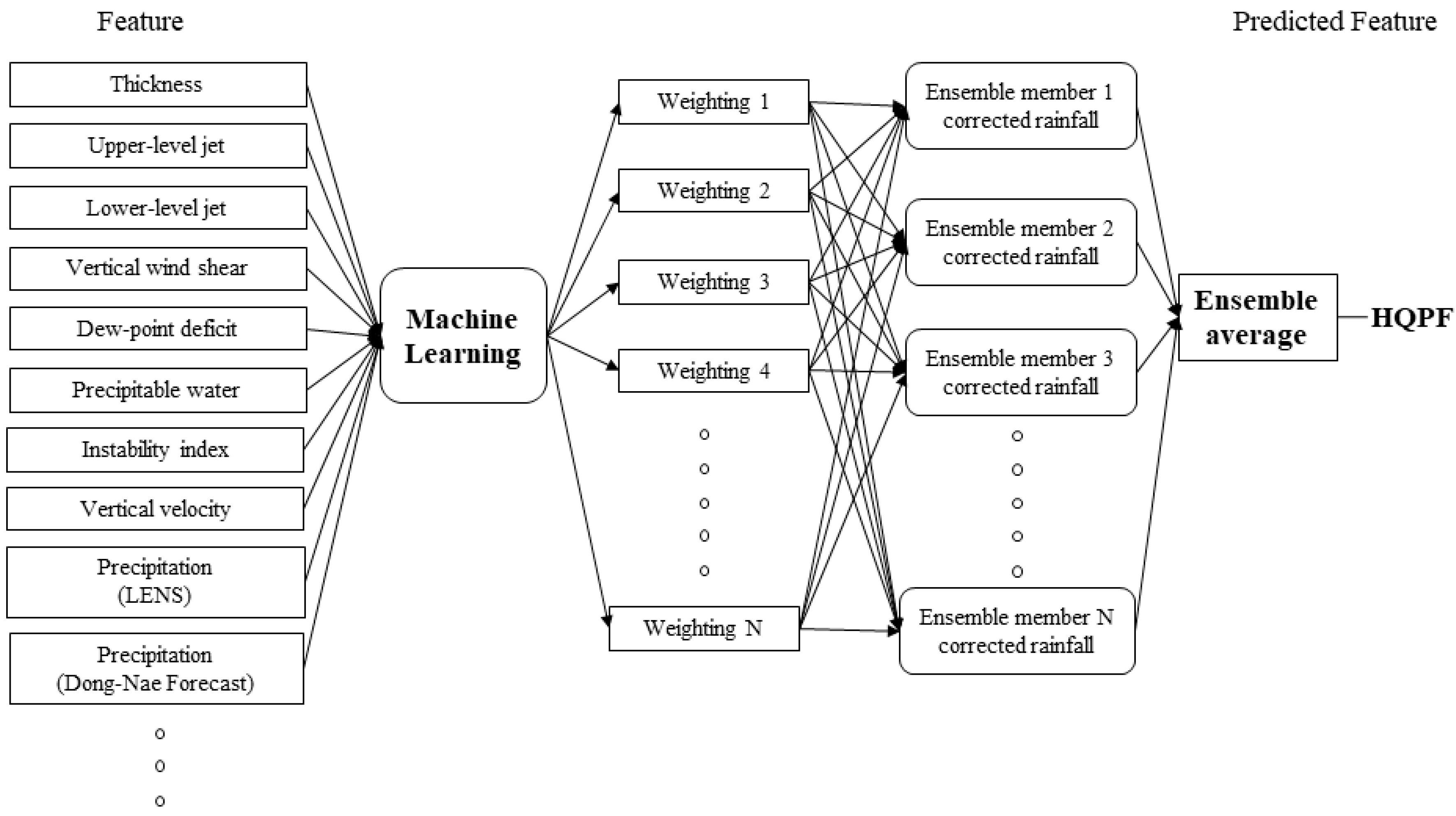
2.2.4. Training
The training for machine learning was conducted using meteorological predictors that had been collected from July to October for the years 2016 and 2017. For the predictors, weights were calculated for rainfall using the XGBoost technique and HQPF was produced by obtaining the average of the ensemble results (
Figure 2).
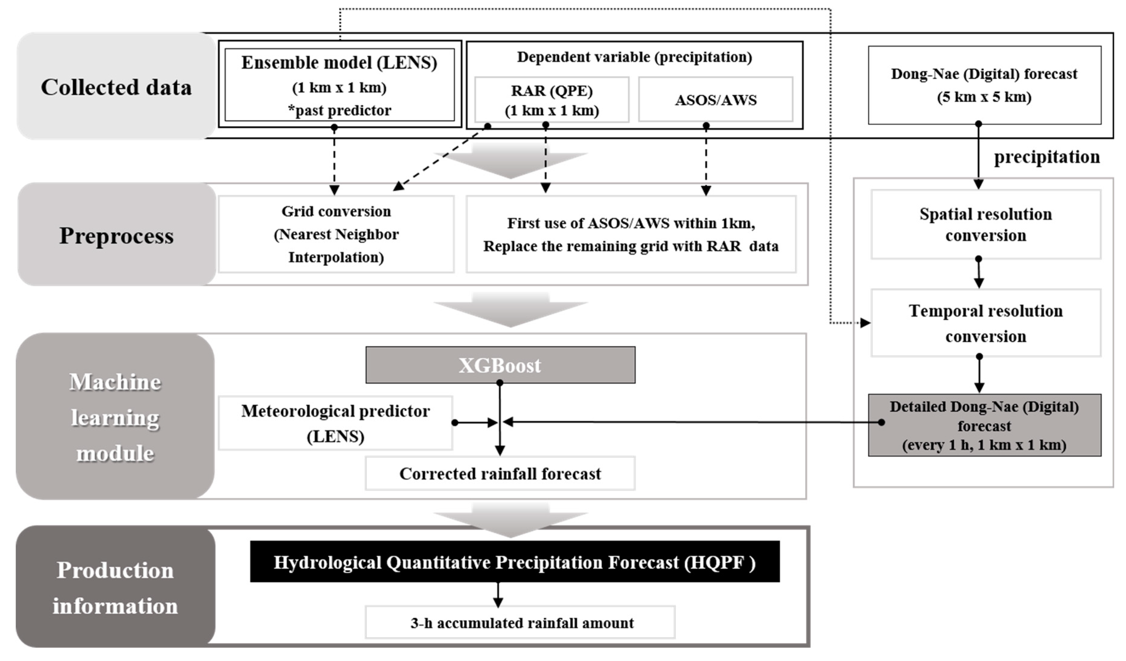
2.2.5. Design of HQPF Algorithm
The HQPF algorithm with rainfall correction was developed through a series of processes, including preprocessing, machine learning, and post-processing, using observation data and numerical forecast data (
Figure 3). The design process was as follows. Preprocessing was the first step to extract meteorological predictors from numerical forecast data that would be used as input data for machine learning. In this step, the meteorological predictors mentioned in
Section 2.1.1 and
Section 2.2.2 were extracted from the weather observation data and forecast data. This step also covered the conversion process of spatial and temporal resolution. The second step, machine learning, was to conduct its training by using the meteorological predictors that had been collected from July to October for the years 2016 and 2017. For the meteorological predictors, the XGBoost of the machine learning technique was applied to produce a 1 h interval of rainfall corrected for each of the ensemble members by inputting the LENS forecast data and Dong-Nae Forecast data. However, the main purpose of HQPF is to provide an improved input for the criteria of precipitation special weather report and heavy rainfall impact model for KMA, which are operated with 3 h interval accumulated rainfall. In this regard, this study focused on the 3 h accumulated rainfall. Lastly, during the post-processing, the corrected rainfall values of the ensemble members were averaged and finally HQPF was calculated.
2.3. Selection of Heavy Rainfall Cases
2.3.1. Case 1: Heavy Rainfall in Seoul
This study used the case of localized heavy rainfall at 13:00 on 28–31 August 2018, in Seoul (
Figure 4). During the period, a special warning for a heat wave was issued over the southern region. Furthermore, the central region, including Seoul, experienced heavy rain, with over 30 mm of rainfall per hour, because it is located between the high- and low-pressure system in the atmosphere. The cold air coming from the north and the North Pacific, which is over the southern part of Japan, collided and, at the same time, the tropical cyclone, which included a large amount of water vapor, was moving into the central region of the Korean peninsula from Taiwan by riding the lower jet stream to form the rain belt stretching from the east to the west over the region (
Figure 4). The radar images of the KMA show there was the rain belt, which stretched from the east to the west with 20 mm or more of rainfall. During that period, there was heavy rainfall, with 60 mm or more per hour in some areas. As shown in
Figure 4 (right), the southern part of Seoul, mostly the Hangang river area, experienced rainfall with 5 mm or less per hour, while in the northern area, heavy rain of 50 mm or more per hour occurred at the same time period. This heavy rain case was characterized by the high deviation across the region and heavy rain in the area north of the Hangang River, Seoul.
In the above radar images, it is shown that localized heavy rain occurred mostly in the area north of the Hangang River, Seoul. Therefore, in this study, four sites of the areas were selected to see the time series for the 1 h accumulated precipitation (
Figure 5). The rainfall information of the four sites, Nowon, Jungnang, Dobong, and Gangnam, is shown in
Table 4. The peak rainfall for Nowon and Jungnang occurred at 18:00 and 19:00 on 28 August with 20.4 mm/h and 31.1 mm/h, respectively. For Dobong, the peak precipitation occurred at 00:00 on 30 August with 76.0 mm/h. The peak precipitation for Gangnam occurred at 21:00 on 28 August with 29.5 mm/h.
The time series characteristics of observed rainfall for Nowon, Jungnang, and Gangnam included heavy rainfall (I), which was followed by the state of weak rainfall (II). For Dobong, after a few hours of heavy rainfall, weak rainfall did not follow. The accumulated rainfall and intensity are shown in
Table 4, with classification for heavy rainfall and, afterward, weak rainfall. In the heavy rainfall sections for Nowon, Jungnang, Dobong, and Gangnam, the accumulated precipitation was 76.0 mm, 74.6 mm, and 309 mm, 57.5 mm, respectively.
2.3.2. Case 2: Typhoon Kong-Rey
The second case study was about the 25th typhoon, Kong-rey, which occurred on 28 September 2018. When the typhoon approached Jeju island on 6 October, its category was medium-scale typhoon (KMA criteria) with 975 hPa central pressure, 32 m/s maximum wind speed, and 350 km strong wind radius. After that, the typhoon headed north and north-east, it landed with 975 hPa central pressure on the Korean peninsula. As shown in
Figure 6, the typhoon brought an intense and narrow rain band with a more than 10 mm per hour rainfall rate due to the influence of the front of the typhoon before landing on the Korean peninsula. Precipitation was particularly concentrated in the northwestern (about 36–37° N, 127° E) and southeastern (about 35° N, 128–130° E) parts of Korea.
2.4. Verification Indicators and Methodologies
This study used three indicators to evaluate the accuracy of the predicted HQPF. The verification indicators included percentage error, mean absolute error (MAE), which indicates the mean error of corrected precipitation, and normalized peak error (NPE), which indicates the maximum error of the predicted HQPF:
In the equation above, is for the observed data, for the corrected precipitation (HQPF), and n for the number of data. and indicate the maximum value of the predicted precipitation and the observed, respectively. Equations (7) and (8) are the percentage error value and MAE, respectively, with a lower value indicating a lower deviation between the prediction and the actual value. Equation (9) is an indicator that shows the error for the maximum precipitation value and is best suited to the study’s purpose in error analysis.
3. Results
3.1. Case 1: Rainfall in Seoul
3.1.1. Spatial Distribution
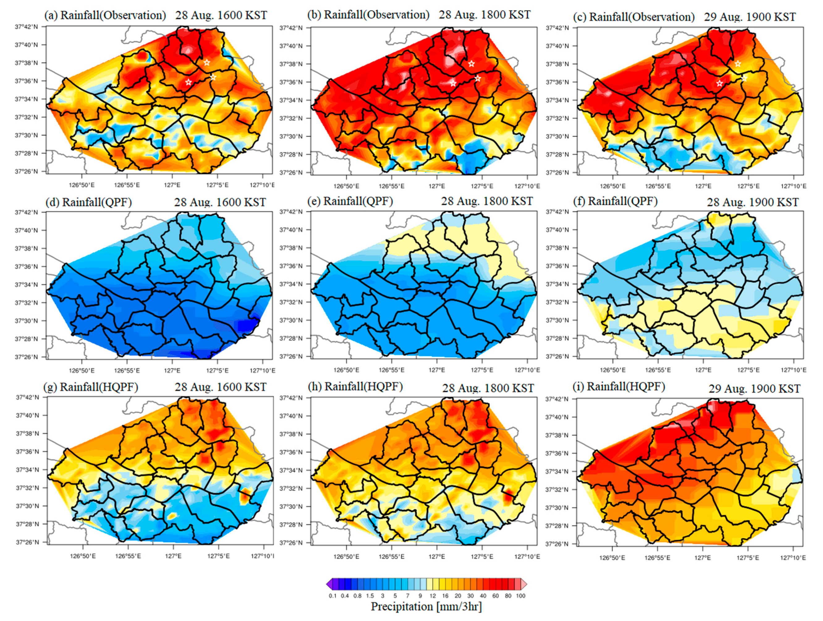
The KMA defines heavy rainfall as precipitation with 60 mm or more of 3 h accumulated precipitation. As shown in
Figure 7a–c, about the spatial distribution of 3 h accumulated precipitation, the heavy rain occurred mainly over the northern part of Seoul. As explained in
Section 2.3, during that period, the heavy rain area covered the Nowon, Jungnang, Dobong, and Gangnam sites (marked with a star in
Figure 7a–c). As shown in
Figure 7d–f, the QPF was not able to forecast heavy rainfall of 10 mm or more per hour. Although, in
Figure 7e,f, the rain rate around 15 mm per hour was predicted for the northern part, but it still had the limitation of forecasting heavy rain. The HQPF forecasting result of
Figure 7g–i shows the heavy rainfall over north Seoul. It simulated the localized heavy rainfall area, which was not the case for the QPF, which suggests that the machine learning enhanced the forecasting performance for localized heavy rainfall.
For the quantitative measure of rainfall accuracy, the percentage error with respect to individual grid points was calculated.
Figure 8 presents the spatial distribution of percentage error derived from QPF-based rainfall and HQPF-based rainfall. Consistent with the comparison of spatial distribution of 3 h accumulated rainfall amount (
Figure 7), the percentage error from HQPF-based rainfall was significantly reduced compared to that from QPF-based rainfall. Regardless of selected timing, errors of more than 80% were predominant in the QPF-based rainfall. In particular, the northern part of Seoul maintained a consistently significant error. On the other hand, HQPF-based rainfall remarkably reduced the amount of error. Although some regions still suffered from large error, the majority of the regions clearly revealed the reduction in error. One notable deficiency was seen in the southern part of Seoul on 29 August. This was because the HQPF tends to overestimate weak precipitation compared to what is observed, which will be further improved by our future study.
3.1.2. Time Series Distribution
In the above analysis on spatial distribution, the localized heavy rainfall occurred mostly over north Seoul; therefore, the study identified the time series for the three sites, Nowon, Jungnang, and Dobong, that represented the north. An additional analysis of Gangnam, which is located in the southern part of Seoul, was conducted for the verification of performance of HQPF. For the time series analysis, we selected the two different time segments that possessed observed peaks. This was because, except for Dobong station, the temporal evolution of rainfall exhibited multiple peaks. Although the skill in simulating the maximum peak is the most important, it is more desirable to capture relatively weak peaks as well. Therefore, data were carried out in two segments to verify the performance of QPF and HQPF. Information on the rainfall shown in
Figure 9 is summarized in
Table 5. The percentage errors for the peak rainfall of the forecasting results of QPF and HQPF in comparison with the observed are provided in
Table 4.
In Nowon, in
Figure 9a, the maximum rainfall was observed at 18:00 on 28 August, with 46 mm/3 h. For the period, rainfall was 10.7 mm/3 h through QPF, whereas 49.3 mm/3 h through HQPF. When calculating the errors in percentage in comparison with the observed, they were 76.7% for QPF and 7.2% for HQPF. In section II for Nowon, the rainfall was 20 mm for QPF and 25.7 mm for HQPF with the percentage errors of 12.3% and 12.7%, respectively.
In section I for Jungnang, 8.9 mm/3 h of rainfall was predicted by QPF, but HQPF predicted a heavier rainfall of 28 mm/3 h. There was underestimation for both the QPF and HQPF, compared to the observed; however, in terms of the percentage error, the HQPF predicted the rainfall twice as accurately as the QPF. In period II for Jungnang, QPF and HQPF produced 17.2 mm/3 h and 14.6 mm/3 h, with the percentage errors of 16.2% and 1.4%, respectively. The difference in the absolute value between the observed and HQPF, which had a lower percent error, was only 0.2 mm/3 h.
Out of the three sites of the study, Dobong recorded the peak precipitation (119.0 mm/3 h). During the study period, QPF predicted 17.2 mm/3 h, which does not satisfy the heavy rainfall definition, and the percentage error was 85.6%. HQPF predicted 180.4 mm/3 h, which satisfies the definition, but was still overestimated, with 51.6% of percentage error.
In Gangnam in
Figure 9d, the maximum rainfall was 3.5 mm/3 h with QPF, but 21.1 mm/3 h through HQPF. When calculating the errors in percentage in comparison with the observed, they were 90.3% for QPF and 41.2% for HQPF. In section II for Gangnam, the rainfall was 24.4 mm for QPF and 31.5 mm for HQPF, with the percentage errors of 43.6% and 27.3%, respectively.
The percentage error for Nowon-II was 12.3% and 12.7% by QPF and HQPF, respectively, which means that the difference between the two is 1% or less in
Table 5 and
Figure 10. However, the difference was identified by a factor from 1.7 times to 11.6 times across the sections. For the maximum rainfall period for each of the sites, Nowon-I showed the percentage error of 75.7% and 7.2% for QPF and HQPF, respectively, with a difference by a factor of 1.6 times. Furthermore, it was 1.9 times and 11.6 times for Jungnang-I and Jungnang-II, respectively. For Dobong-I, the percentage error of QPF and HQPF was 85.6% and 51.6%, respectively, with a difference by a factor of 1.7 times. As a result, for the peak rainfall, HQPF improved the error by up to 11.6 times from the level of QPF. It was 2.2 times and 1.6 times for Gangnam-I and Gangnam-II, respectively.
3.1.3. Analysis of Statistical Error
For the rainfall correction results to be used for hydrological purposes, the evaluation should be conducted with a focus on the period of localized heavy rainfall (rainfall section I). Therefore, in
Section 3.1.3, statistical verification is made for the MAE and NPE, and the result is summarized in
Table 6 and
Table 7.
The MAE result was 18.6 mm/3 h, 19.4 mm/3 h, 48.7 mm/3 h, and 19.1 mm/3 h through QPF and 13.6 mm/3 h, 14.2 mm/3 h, 33.3 mm/3 h, and 12.0 mm/3 h through HQPF, for Nowon, Jungnang, Dobong, and Gangnam, respectively. For all four sites, HQPF showed a lower error than QPF, and the difference between QPF and HQPF was 5.0 mm/3 h for Nowon, 5.2 mm/3 h for Jungnang, 15.4 mm/3 h for Dobong, and 7.1 mm/3 h for Gangnam.
As shown in
Table 7, all NPEs of QPF had a negative value, with −0.77, −0.82, −0.85, and −0.90, respectively, for Nowon, Jungnang, Dobong, and Gangnam, indicating the underestimation made for rainfall in comparison with the observed. The NPEs of HQPF were 0.07, −0.43, 0.52, and −0.41, respectively, which means an underestimation for Jungnang and Gangnam and overestimation for Nowon and Dobong. Furthermore, regarding the NPE range of QPF and HQPF, QPF showed errors ranging from 0.77 to 0.90, while HQPF was from 0.07 to 0.52. As a result, considering that the values close to zero (0) have a higher similarity with the observed, the study found an enhanced forecast performance for localized heavy rainfall from the HQPF’s results, which were produced through machine learning.
3.2. Case 2: Typhoon Kong-Rey (1825)
In this chapter, we analyzed the amount of precipitation that fell on the Korean Peninsula during Typhoon Kong-rey. As seen in radar images (see
Figure 6), Typhoon Kong-rey brought a very intense and localized rain band, which can provide a good opportunity to compare the accuracy of the rainfall forecast from the QPF raw output and the HQPF corrected output. Using the observations, the distribution of precipitation on the Korean Peninsula was compared (
Section 3.2.1), and the performance of QPF and HQPF was verified by selecting four observation stations (
Section 3.2.2).
3.2.1. Spatial Distribution
In the spatial distribution of the observed precipitation, as shown in
Figure 11a–c, one can see that the rain bands exist in the northwest (Gyeonggi, Chungcheong, and Jeolla provinces) and the southeast of Korea. In the spatial distribution of QPF in
Figure 11e,f, precipitation in Jeju Island was not simulated at 0700 KST and 0800 KST, and the precipitation area of more than 10 mm/3 h in Gyeonggi Province was smaller than observed. In
Figure 11g–i, a precipitation distribution similar to observation was found in Chungcheng and northern Jeolla Province at 0600 KST and 0700 KST. In particular, at 0800 KST, HQPF simulated precipitation in Gyeonggi Province, including Seoul and southeastern Korea, while QPF failed to simulate precipitation.
3.2.2. Analysis of Statistical Error
For the four stations shown in
Figure 1b, this study investigated the location, time, and amount of maximum precipitation in the observations (
Figure 12). At all stations, it was obvious that the maximum precipitation occurred on 6 October, and the observed times of the maximum rainfall were 06:00 in Dangjin, Seosan, and Taean and 09:00 at Bamsagol station. The maximum precipitation accumulated over the three-hour period was 36 mm (Dangjin), 48 mm (Baemsagol), 33.8 mm (Seosan), and 33 mm (Taean) (
Table 8).
The maximum precipitation was investigated for QPF and HQPF during the typhoon (21:00 5 October–21:00 7 October). As shown in
Table 9, the maximum precipitation values of QPF were 8.3, 22.6, 8.9, and 9 mm, respectively, for Dangjin, Bamsagol, Seosan and Taean. The values of HQPF were 17.5, 48.6, 21.8, and 17.4 mm, respectively.
As shown in
Table 10, all NPEs of QPF had a negative value, with −0.77, −0.53, −0.74, and −0.73, respectively, for Dangjin, Bamsagol, Seosan, and Taean, indicating the underestimation made for rainfall in comparison with the observed. The NPEs of HQPF were −0.51, 0.01, −0.36, and −0.47, respectively, and these mean an underestimation for Dangjin, Seosan, Taean and overestimation for Bamsagol. Furthermore, regarding the NPE range of QPF and HQPF, QPF showed errors ranging from 0.53 to 0.77, while HQPF showed errors from 0.01 to 0.51. As a result, this section found an enhanced forecast performance during Typhoon Kong-rey from HQPF’s results, which were produced through machine learning, as in case 1.
4. Discussion
This study developed a machine learning-based rainfall correction technique for Seoul and, its results were compared with the observed results. The study aimed to predict an absolute value of the observed rainfall for a heavy rainfall period. HQPF had a better performance than QPF in predicting rainfall for a heavy rainfall period. When compared with QPF, HQPF used the same data but it reflected the learning, which was the results from past rainfall cases, through the machine learning, for the rainfall correction. Therefore, HQPF is able to predict in a better and quicker way by using big data-based information, which has a nonlinear relationship, at the same time considering the complex process of rainfall. In particular, the effective provision of heavy rainfall information using HQPF will efficiently support the measures for public facilities and disaster prevention in downtowns.
Regarding the performance of predicting localized rainfall, HQPF provided a better result than QPF, but there was still a limitation, which was the difference in the rainfall area between the observed and the predicted. It is normal that such limitation is experienced in forecasting for localized heavy rainfall that occurs by a complex interaction of mid-scale convective system and synoptic-scale forcing. However, efforts are required to improve the spatial prediction and overcome the limitations.
Machine learning-based HQPF is to reduce the uncertainty of rainfall forecasting information, as shown in the case of Typhoon Kong-rey, which showed the results of HQPF to be better than QPF. However, even in this case, precipitation peak values were not corrected rather than observed rainfall. The first reason for this is that the input data of big data-based machine learning requires sufficient weather input data, but the weather input data used in this study were limited. The second reason is that the basic research on the parameter optimization of machine learning is insufficient. Therefore, in order to obtain an improved machine learning-based HQPF, it is suggested that study of machine learning parameter optimization should be preceded with sufficient weather input data for machine learning.
5. Conclusions
This study applied the machine learning technique to diverse rainfall data provided by the KMA, for the purpose of generating hydrological rainfall information. To develop the HQPF, the study used the ensemble numerical model data, radar data, station observation data, and Dong-Nae Forecast rainfall data, which were provided by the KMA. The data went through a preprocessing step for the conversion to obtain the same level of temporal and spatial resolutions. By analyzing the predictors, the study obtained the final predictors for machine learning. The machine learning that the study used to consider the processing speed and expandability was XGBoost. Lastly, before the post-processing to produce the final correction rainfall, the average was obtained for correction rainfall by ensemble members that calculated through machine learning.
To evaluate the accuracy of HQPF’s prediction applied with machine learning, the study targeted the representative heavy rainfall cases of the Seoul area and typhoon Kong-rey (1825) in 2018. As a result of analyzing the spatial field, unlike QPF, HQPF was able to simulate the localized heavy rainfall area, indicating that the machine learning enhanced the performance of predicting localized heavy rainfall. In addition, as a result of analyzing the MAEs for four sites, the MAEs of QPF were 18.6 mm/3 h (Nowon), 19.4 mm/3 h (Jungnang), 48.7 mm/3 h (Dobong), and 19.1 mm/3 h (Gangnam), while the MAEs of HQPF were 13.6 mm/3 h (Nowon), 14.2 mm/3 h (Jungnang), 33.3 mm/3 h (Dobong), and 12.0 mm/3 h (Gangnam), which indicates that the error became lower for all the sites by HQPF. Regarding the NPEs, QPF had −0.77 (Nowon), and −0.82 (Jungnang), −0.85 (Dobong), and −0.90 (Gangnam), while HQPF had 0.07 (Nowon), −0.43 (Jungnang), 0.52 (Dobong), and −0.41 (Gangnam). Regarding the NPEs during typhoon Kong-rey, QPF had −0.77 (Dangjin), −0.53 (Bamsagol), −0.74 (Seosan), and −0.73 (Taean), while HQPF had −0.51 (Dangjin), 0.01 (Bamsagol), −0.36 (Seosan), and −0.47 (Taean). This provides clear evidence that the rainfall correction algorithm improved rainfall information.
Although a significant improvement was made for rainfall information by the rainfall correction algorithm that the study developed, limitations still remain in terms of predicting the peak precipitation and defining areas for rainfall forecasting. Therefore, conducting additional studies is necessary for rainfall types, preceding predictors, and the application of more localized rainfall cases to develop algorithms, producing correction rainfall in a more accurate and efficient way.
Based on the results, additional analyses can be made in the future for diverse heavy rainfall cases to use machine learning for the advancement of the rainfall correction technique. HQPF is expected to contribute to flood predictions and impact forecasts [
11,
12] and can be utilized as useful data in a wide range of hydrological research fields.


