Subseasonal Influences of Teleconnection Patterns on the Boreal Wintertime Surface Air Temperature over Southern China as Revealed from Three Reanalysis Datasets


Abstract
:1. Introduction
2. Data and Methods
2.1. Data and Processing
2.2. Methods
2.2.1. Teleconnection Patterns
2.2.2. Daily Indices of Teleconnection Patterns
2.2.3. Effective Sample Size
2.2.4. Significance Test
3. Results
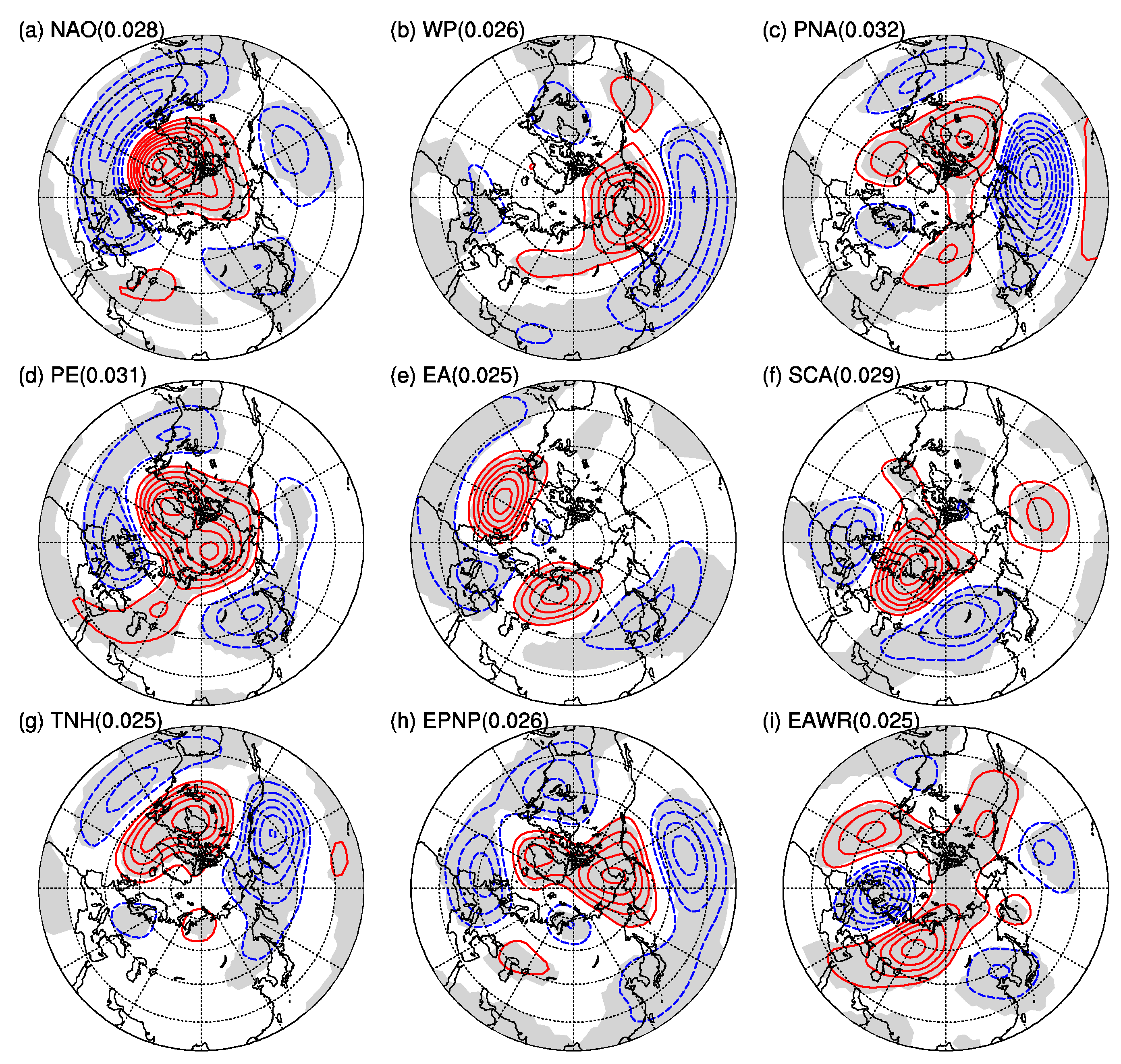
3.1. Comparison of Teleconnection Patterns Revealed by Different Datasets
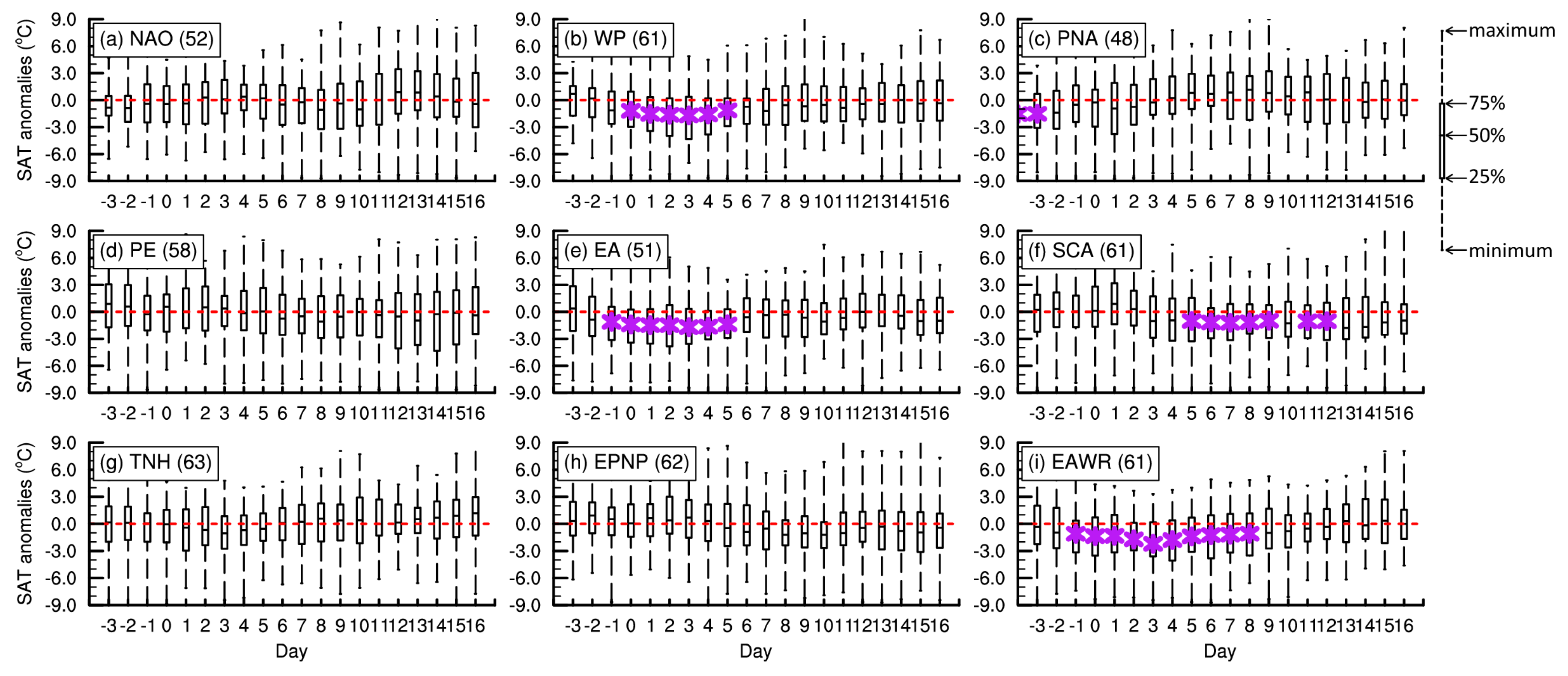
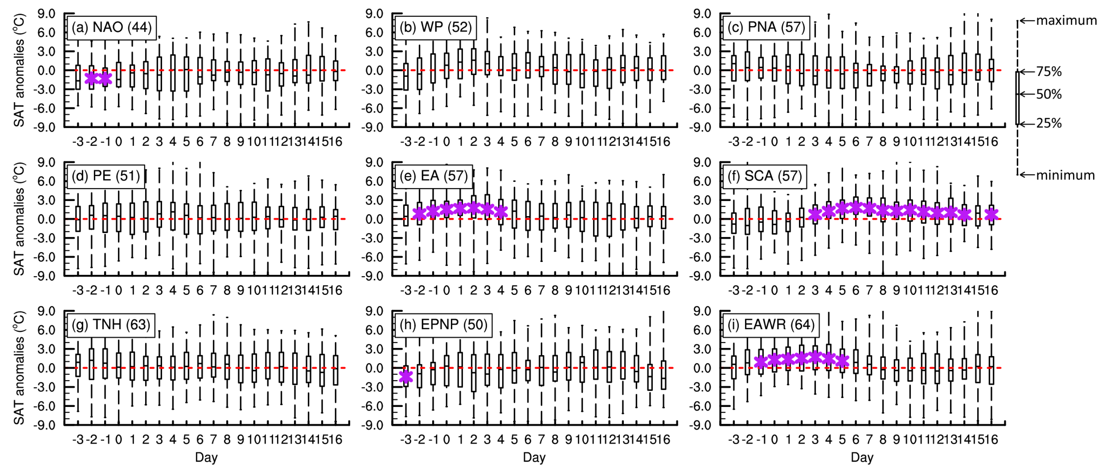
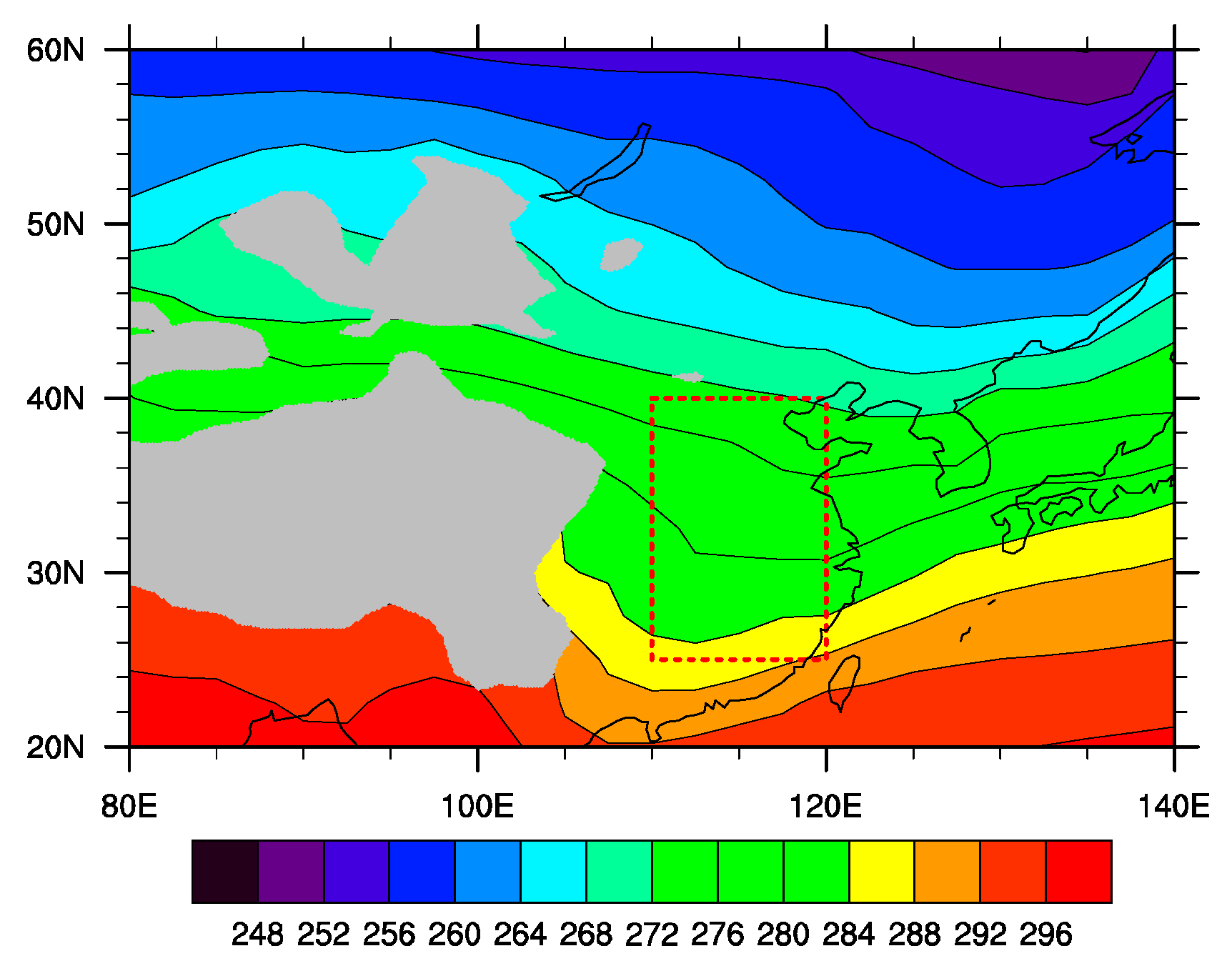
3.2. Relationship with Area-Averaged SAT Over Southern China
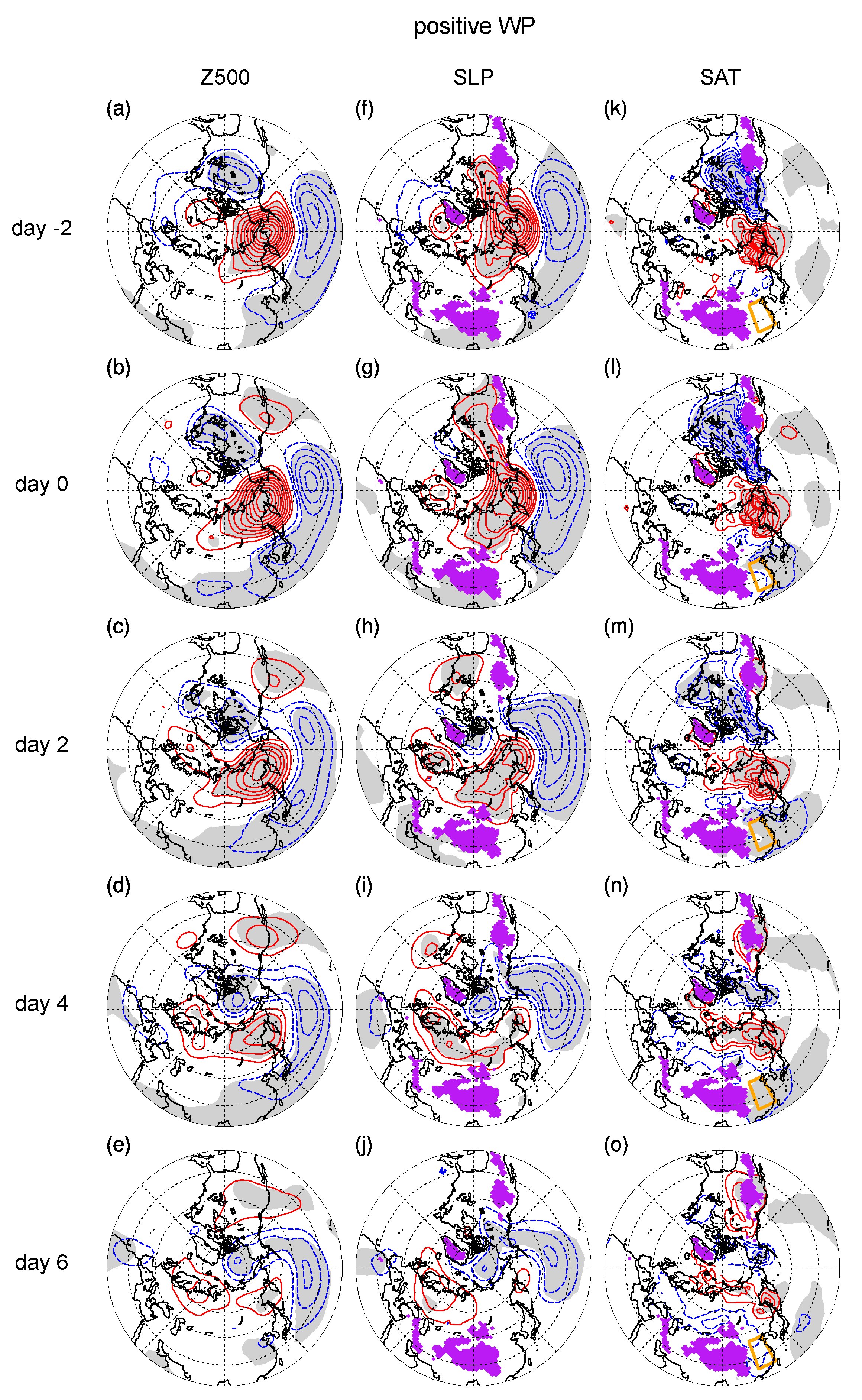
3.3. Circulation Evolution
3.3.1. WP Events
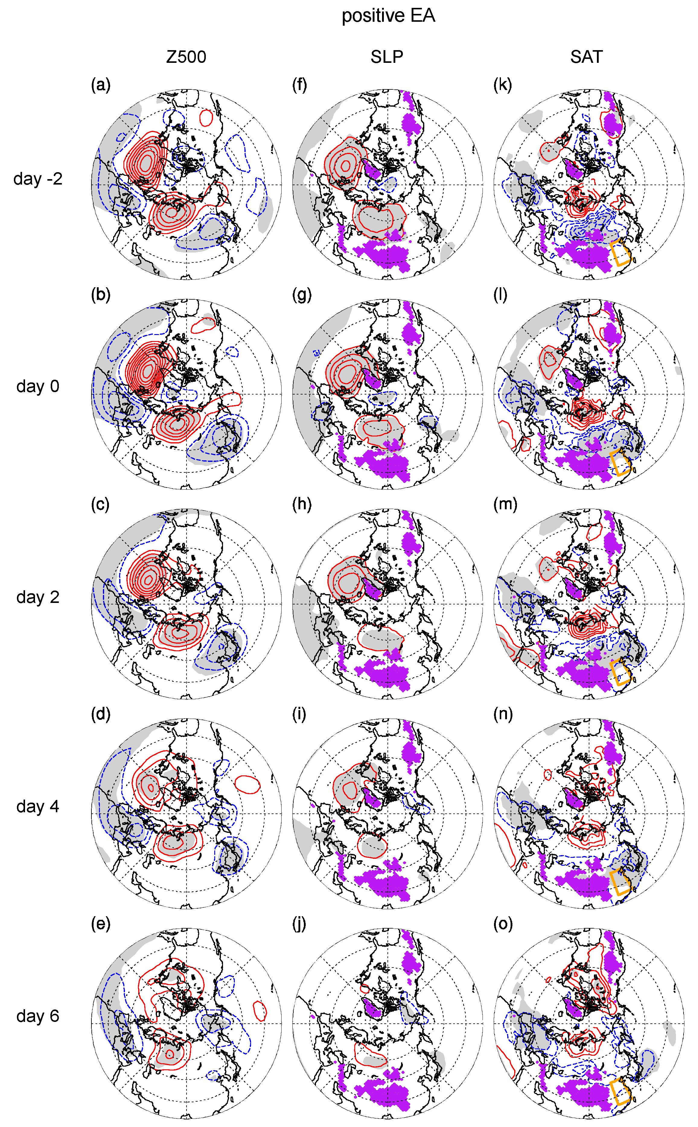
3.3.2. EA Events
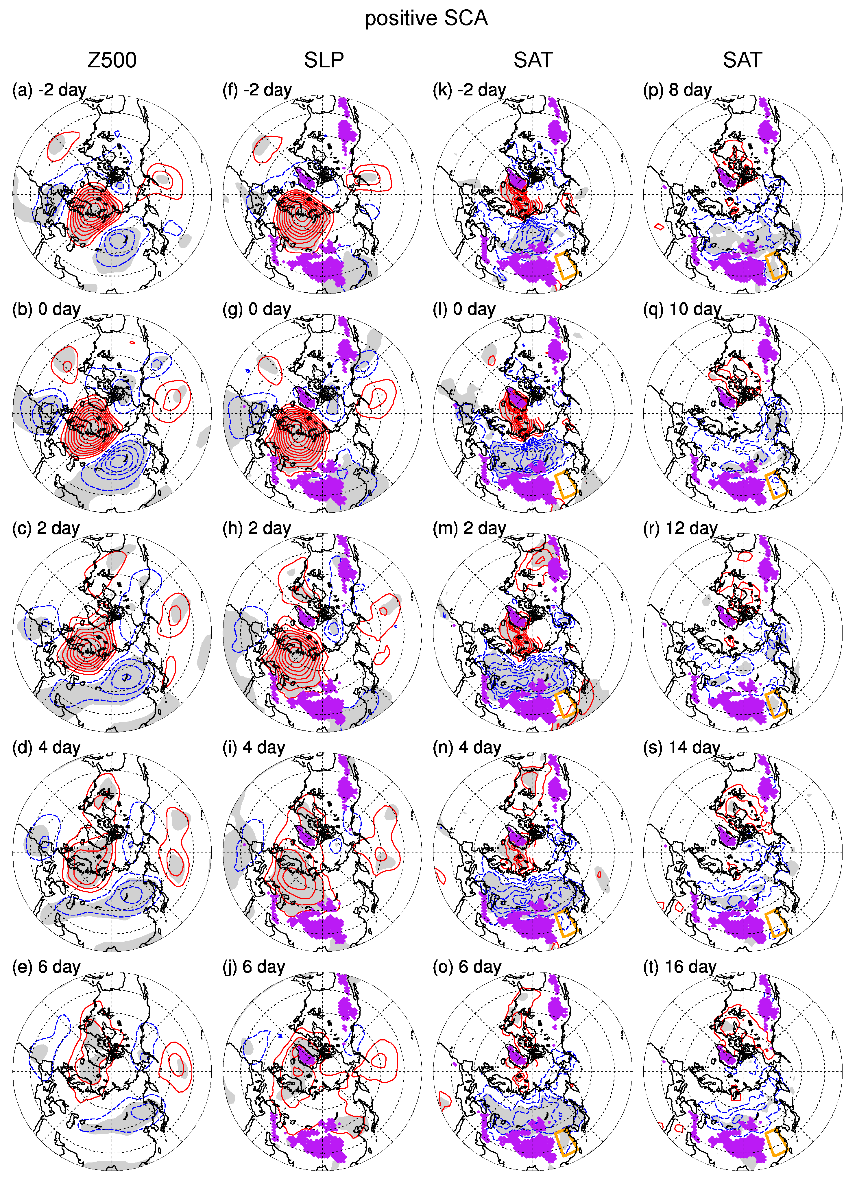
3.3.3. SCA Events
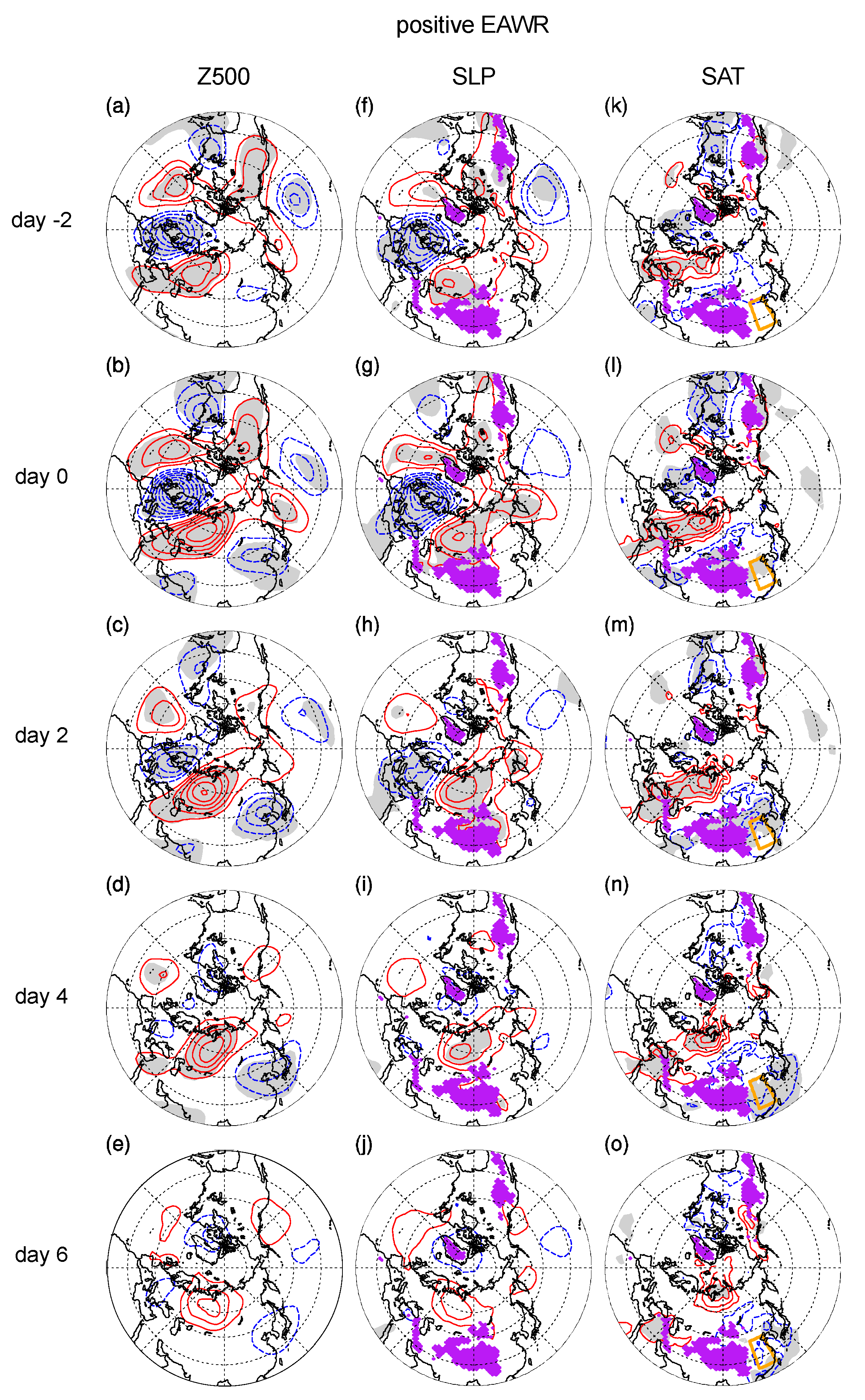
3.3.4. EAWR Events
4. Discussion
5. Conclusions
Author Contributions
Funding
Acknowledgments
Conflicts of Interest
References
- Wallace, J.M.; Gutzler, D.S. Teleconnections in the geopotential height field during the Northern Hemisphere winter. Mon. Weather Rev. 1981, 109, 784–812. [Google Scholar] [CrossRef]
- Horel, J. A rotated principal component analysis of the interannual variability of the Northern Hemisphere 500 mb height field. Mon. Weather Rev. 1981, 109, 2080–2092. [Google Scholar] [CrossRef]
- Barnston, A.G.; Livezey, R.E. Classification, Seasonality and Persistence of Low-Frequency Atmospheric Circulation Patterns. Mon. Weather Rev. 1987, 115, 1083–1126. [Google Scholar] [CrossRef]
- Lau, N.-C. Variability of the observed midlatitude storm tracks in relation to low-frequency changes in the circulation pattern. J. Atmos. Sci. 1988, 45, 2718–2743. [Google Scholar] [CrossRef]
- Athanasiadis, P.J.; Wallace, J.M.; Wettstein, J.J. Patterns of wintertime jet stream variability and their relation to the storm tracks. J. Atmos. Sci. 2010, 67, 1361–1381. [Google Scholar] [CrossRef]
- Blackmon, M.L.; Lee, Y.H.; Wallace, J.M. Horizontal structure of 500 mb height fluctuations with long, intermediate and short time scales. J. Atmos. Sci. 1984, 41, 961–980. [Google Scholar] [CrossRef]
- Nakamura, H.; Tanaka, M.; Wallace, J.M. Horizontal structure and energetics of Northern Hemisphere wintertime teleconnection patterns. J. Atmos. Sci. 1987, 44, 3377–3391. [Google Scholar] [CrossRef]
- Frederiksen, J.S. A unified three-dimensional instability theory of the onset of blocking and cyclogenesis. II: Teleconnection Patterns. J. Atmos. Sci. 1983, 40, 2593–2609. [Google Scholar] [CrossRef]
- Simmons, A.J.; Wallace, J.M.; Branstator, G.W. Barotropic Wave Propagation and Instability, and Atmospheric Teleconnection Patterns. J. Atmos. Sci. 1983, 40, 1363–1392. [Google Scholar] [CrossRef]
- Feldstein, S.B. Fundamental mechanisms of the growth and decay of the PNA teleconnection pattern. Quart. J. Roy. Meteor. Soc. 2002, 128, 775–796. [Google Scholar] [CrossRef] [Green Version]
- Tanaka, S.; Nishii, K.; Nakamura, H. Vertical structure and energetics of the Western Pacific teleconnection pattern. J. Clim. 2016, 29, 6597–6616. [Google Scholar] [CrossRef]
- Hoskins, B.J.; Karoly, D.J. The steady linear response of a spherical atmosphere to thermal and orographic forcing. J. Atmos. Sci. 1981, 38, 1179–1196. [Google Scholar] [CrossRef]
- Bueh, C.; Nakamura, H. Scandinavian pattern and its climatic impact. Quart. J. Roy. Meteor. Soc. 2007, 133, 2117–2131. [Google Scholar] [CrossRef]
- Tan, B.; Yuan, J.; Dai, Y.; Feldstein, S.B.; Lee, S. The linkage between the Eastern Pacific teleconnection pattern and convective heating over the tropical Western Pacific. J. Clim. 2015, 28, 5783–5794. [Google Scholar] [CrossRef]
- Branstator, G. The Maintenance of Low-Frequency Atmospheric Anomalies. J. Atmos. Sci. 1992, 49, 1924–1946. [Google Scholar] [CrossRef] [Green Version]
- Wang, N.; Zhang, Y. Evolution of Eurasian teleconnection pattern and its relationship to climate anomalies in China. Clim. Dyn. 2014, 44, 1017–1028. [Google Scholar] [CrossRef] [Green Version]
- Zhang, Y.; Sperber, K.R.; Boyle, J.S. Climatology and Interannual Variation of the East Asian Winter Monsoon: Results from the 1979–95 NCEP/NCAR Reanalysis. Mon. Weather Rev. 1997, 125, 2605–2619. [Google Scholar] [CrossRef]
- Takaya, K.; Nakamura, H. Mechanisms of Intraseasonal Amplification of the Cold Siberian High. J. Atmos. Sci. 2005, 62, 4423–4440. [Google Scholar] [CrossRef]
- Takaya, K.; Nakamura, H. Geographical Dependence of Upper-Level Blocking Formation Associated with Intraseasonal Amplification of the Siberian High. J. Atmos. Sci. 2005, 62, 4441–4449. [Google Scholar] [CrossRef]
- Gong, D.; Wang, S.; Zhu, J. East Asian winter monsoon and Arctic Oscillation. Geophys. Res. Lett. 2001, 28, 2073–2076. [Google Scholar] [CrossRef]
- Takaya, K.; Nakamura, H. Interannual Variability of the East Asian Winter Monsoon and Related Modulations of the Planetary Waves. J. Clim. 2013, 26, 9445–9461. [Google Scholar] [CrossRef]
- Wang, L.; Chen, W. An Intensity Index for the East Asian Winter Monsoon. J. Clim. 2014, 27, 2361–2374. [Google Scholar] [CrossRef]
- Cheung, H.H.N.; Zhou, W. Simple Metrics for Representing East Asian Winter Monsoon Variability: Urals Blocking and Western Pacific Teleconnection Patterns. Adv. Atmos. Sci. 2016, 33, 695–705. [Google Scholar] [CrossRef]
- Feldstein, S.B. The timescale, power spectra, and climate noise properties of teleconnection patterns. J. Clim. 2000, 13, 4430–4440. [Google Scholar] [CrossRef]
- Yuan, J.; Tan, B.; Feldstein, S.B.; Lee, S. Wintertime North Pacific Teleconnection Patterns: Seasonal and Interannual Variability. J. Clim. 2015, 28, 8247–8263. [Google Scholar] [CrossRef] [Green Version]
- Ding, Y. Build-up, air mass transformation and propagation of Siberian high and its relations to cold surge in East Asia. Meteorol. Atmos. Phys. 1990, 44, 281–292. [Google Scholar] [CrossRef]
- Liu, Y.; Lin, W.; Wen, Z.; Wen, C. Three Eurasian teleconnection patterns: Spatial structures, temporal variability, and associated winter climate anomalies. Clim. Dyn. 2014, 42, 2817–2839. [Google Scholar] [CrossRef]
- Zhou, W.; Chan, J.C.L.; Chen, W.; Ling, J.; Pinto, J.G.; Shao, Y. Synoptic-Scale Controls of Persistent Low Temperature and Icy Weather over Southern China in January 2008. Mon. Weather Rev. 2009, 137, 3978–3991. [Google Scholar] [CrossRef] [Green Version]
- Bueh, C.; Shi, N.; Xie, Z. Large-scale circulation anomalies associated with persistent low temperature over Southern China in January 2008. Atmos. Sci. Lett. 2011, 12, 273–280. [Google Scholar] [CrossRef]
- Peng, J.B.; Bueh, C. Precursory Signals of Extensive and Persistent Extreme Cold Events in China. Atmos. Ocean. Sci. Lett. 2012, 5, 252–257. [Google Scholar]
- Hsu, H.-H. Propagation of Low-Level Circulation Features in the Vicinity of Mountain Ranges. Mon. Weather Rev. 1987, 115, 1864–1893. [Google Scholar] [CrossRef] [Green Version]
- Dee, D.P.; Uppala, S.M.; Simmons, A.J.; Berrisford, P.; Poli, P.; Kobayashi, S.; Andrae, U.; Balmaseda, M.A.; Balsamo, G.; Bauer, P.; et al. The ERA-Interim reanalysis: Configuration and performance of the data assimilation system. Quart. J. Roy. Meteor. Soc. 2011, 137, 553–597. [Google Scholar] [CrossRef]
- Kalnay, E.; Kanamitsu, M.; Kistler, R.; Collins, W.; Deaven, D.; Gandin, L.; Iredell, M.; Saha, S.; White, G.; Woollen, J.; et al. The NCEP/NCAR 40-year reanalysis project. Bull. Amer. Meteor. Soc. 1996, 77, 437–470. [Google Scholar] [CrossRef]
- Kobayashi, S.; Ota, Y.; Harada, Y.; Ebita, A.; Moriya, M.; Onoda, H.; Onogi, K.; Kamahori, H.; Kobayashi, C.; Endo, H.; et al. The JRA-55 Reanalysis: General Specifications and Basic Characteristics. J. Meteorol. Soc. Jpn. 2015, 93, 5–48. [Google Scholar] [CrossRef] [Green Version]
- Yang, S.; Lau, K.M.; Kim, K.M. Variations of the East Asian Jet Stream and Asian-Pacific-American Winter Climate Anomalies. J. Clim. 2002, 15, 306–325. [Google Scholar] [CrossRef]
- Baldwin, M.P.; Dunkerton, T.J. Stratospheric Harbingers of Anomalous Weather Regimes. Science 2001, 294, 581–584. [Google Scholar] [CrossRef] [PubMed]
- Wilks, D.S. “The Stippling Shows Statistically Significant Grid Points”: How Research Results are Routinely Overstated and Overinterpreted, and What to Do about It. Bull. Amer. Meteor. Soc. 2016, 97, 2263–2273. [Google Scholar] [CrossRef]
- Walker, G.T.; Bliss, E.W. World weather V. Mem. Roy. Meteor. Soc. 1932, 4, 53–84. [Google Scholar]
- Rogers, J.C. The North Pacific Oscillation. J. Climate 1981, 1, 39–57. [Google Scholar] [CrossRef]
- Linkin, M.E.; Nigam, S. The North Pacific Oscillation–West Pacific Teleconnection Pattern: Mature-Phase Structure and Winter Impacts. J. Clim. 2008, 21, 1979–1997. [Google Scholar] [CrossRef]
- Hoskins, B.J.; McIntyre, M.E.; Robertson, A.W. On the use and significance of isentropic potential vorticity maps. Quart. J. Roy. Meteor. Soc. 1985, 111, 877–946. [Google Scholar] [CrossRef]
- Crasemann, B.; Handorf, D.; Jaiser, R.; Dethloff, K.; Nakamura, T.; Ukita, J.; Yamazaki, K. Can preferred atmospheric circulation patterns over the North-Atlantic-Eurasian region be associated with arctic sea ice loss? Polar Sci. 2017, 14. [Google Scholar] [CrossRef]
- Dai, Y.; Tan, B. Two Types of the Western Pacific Pattern, Their Climate Impacts, and the ENSO Modulations. J. Clim. 2019, 32, 823–841. [Google Scholar] [CrossRef]
- Luo, D.; Xiao, Y.; Diao, Y.; Dai, A.; Franzke, C.L.E.; Simmonds, I. Impact of Ural Blocking on Winter Warm Arctic–Cold Eurasian Anomalies. Part II: The Link to the North Atlantic Oscillation. J. Clim. 2016, 29, 3949–3971. [Google Scholar] [CrossRef]


| EM | ERA-Interim | JRA | NCEP/NCAR | |||||||||
|---|---|---|---|---|---|---|---|---|---|---|---|---|
| Mode | Mode | Mode | Mode | |||||||||
| NAO | 1 | 8.52 | 9 | 2 | 8.59 | 9 | 4 | 7.53 | 9 | 4 | 7.69 | 9 |
| WP | 3 | 8.21 | 7 | 1 | 8.59 | 7 | 1 | 8.79 | 8 | 2 | 8.26 | 7 |
| PNA | 4 | 7.90 | 9 | 4 | 7.66 | 9 | 3 | 7.87 | 9 | 3 | 7.94 | 10 |
| PE | 5 | 6.64 | 9 | 5 | 6.91 | 9 | 5 | 7.11 | 9 | 5 | 7.12 | 9 |
| EA | 6 | 6.41 | 8 | 7 | 6.12 | 8 | 7 | 6.15 | 8 | 8 | 6.02 | 7 |
| SCA | 7 | 6.31 | 7 | 6 | 6.48 | 7 | 6 | 6.39 | 7 | 7 | 6.12 | 7 |
| TNH | 8 | 5.77 | 6 | 8 | 5.87 | 6 | 8 | 6.13 | 6 | 6 | 6.12 | 6 |
| EPNP | 9 | 5.29 | 6 | 10 | 5.17 | 6 | 10 | 5.06 | 7 | 10 | 5.11 | 6 |
| EAWR | 10 | 4.98 | 6 | 9 | 5.25 | 6 | 9 | 5.21 | 6 | 9 | 5.36 | 6 |
| r (EM, ERA) | r (EM, JRA) | r (EM, NCEP/NCAR) | |
|---|---|---|---|
| NAO | 0.996 | 0.992 | 0.993 |
| WP | 0.995 | 0.992 | 0.997 |
| PNA | 0.996 | 0.965 | 0.985 |
| PE | 0.994 | 0.993 | 0.994 |
| EA | 0.991 | 0.936 | 0.942 |
| SCA | 0.996 | 0.980 | 0.993 |
| TNH | 0.982 | 0.979 | 0.987 |
| EPNP | 0.921 | 0.838 | 0.933 |
| EAWR | 0.989 | 0.910 | 0.931 |
© 2019 by the authors. Licensee MDPI, Basel, Switzerland. This article is an open access article distributed under the terms and conditions of the Creative Commons Attribution (CC BY) license (http://creativecommons.org/licenses/by/4.0/).
Share and Cite
Shi, N.; Zhang, D.; Wang, Y.; Tajie, S. Subseasonal Influences of Teleconnection Patterns on the Boreal Wintertime Surface Air Temperature over Southern China as Revealed from Three Reanalysis Datasets. Atmosphere 2019, 10, 514. https://doi.org/10.3390/atmos10090514
Shi N, Zhang D, Wang Y, Tajie S. Subseasonal Influences of Teleconnection Patterns on the Boreal Wintertime Surface Air Temperature over Southern China as Revealed from Three Reanalysis Datasets. Atmosphere. 2019; 10(9):514. https://doi.org/10.3390/atmos10090514
Chicago/Turabian StyleShi, Ning, Dongdong Zhang, Yicheng Wang, and Suolang Tajie. 2019. "Subseasonal Influences of Teleconnection Patterns on the Boreal Wintertime Surface Air Temperature over Southern China as Revealed from Three Reanalysis Datasets" Atmosphere 10, no. 9: 514. https://doi.org/10.3390/atmos10090514