IonoSeis: A Package to Model Coseismic Ionospheric Disturbances

 , , , , and
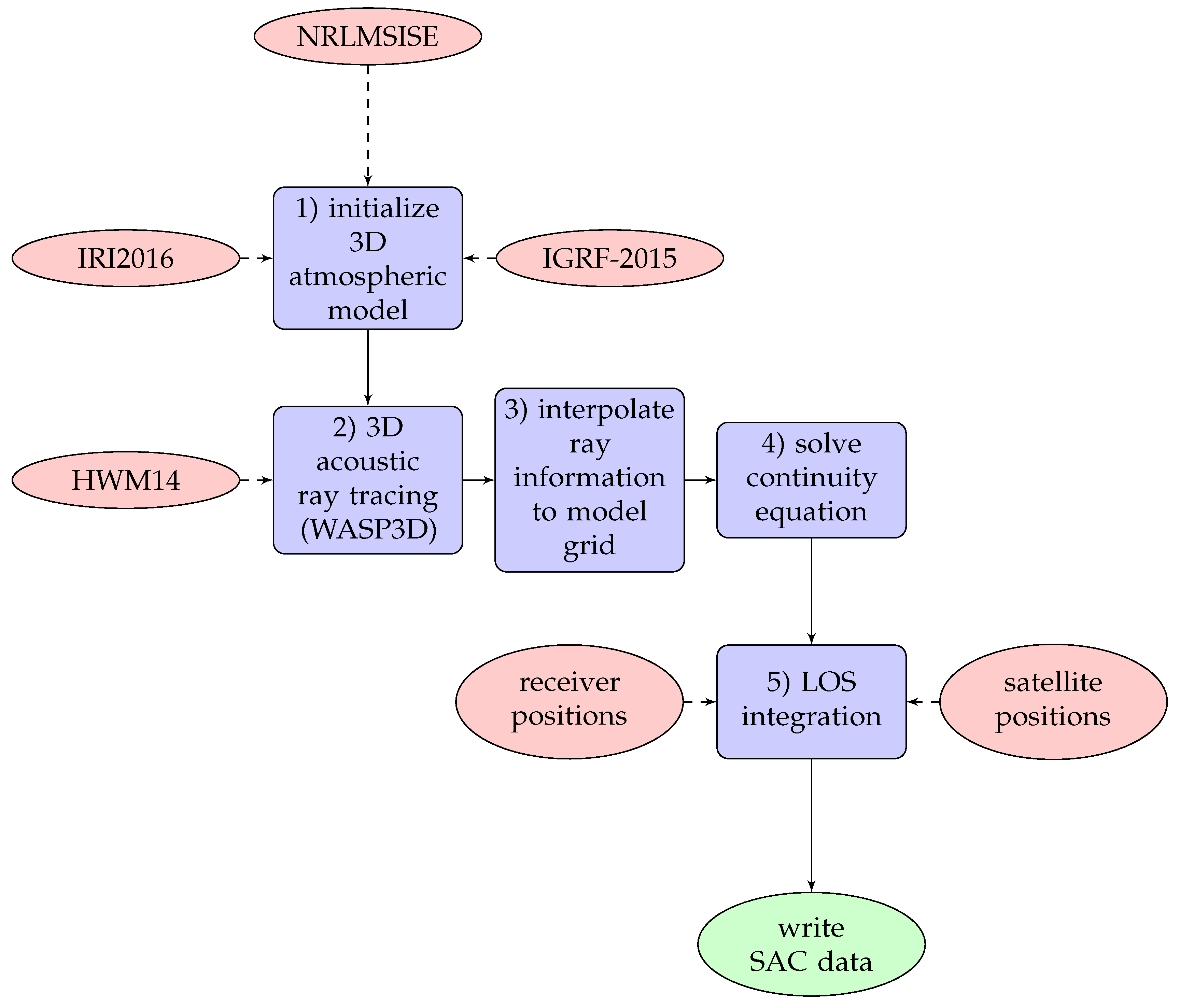
Abstract
:1. Introduction
2. Materials and Methods
2.1. sTEC Observation Data
2.2. The Electron Density Model
- modeling the background electron density (); and
- modeling local perturbations () due to transient phenomena.
2.2.1. The Background Ionosphere
2.2.2. The Coseismic Ionospheric Perturbation
2.2.3. The Geomagnetic Field
2.3. The Neutral Particle Velocity
3. Results
- Create the model domain—build a 3D grid in the atmosphere that contains background electron density and geomagnetic field parameters → save to a NetCDF file.
- For a given epicenter location, run WASP3D over many rays (azimuths and take-off angles) to model the arrival time, the amplitude, and the wavevector of the acoustic wave.
- Interpolate the ray parameters to the atmosphere grid → create a single NetCDF file with all necessary parameters.
- Solve Equation (5) using time integration—create a NetCDF file with the electron density perturbations () at each time step.
- Perform LOS integration for a given receiver and satellite pair—create SAC formatted data files that contain the LOS integration for both the background TEC and the CIP TEC (i.e., Equation (3)).
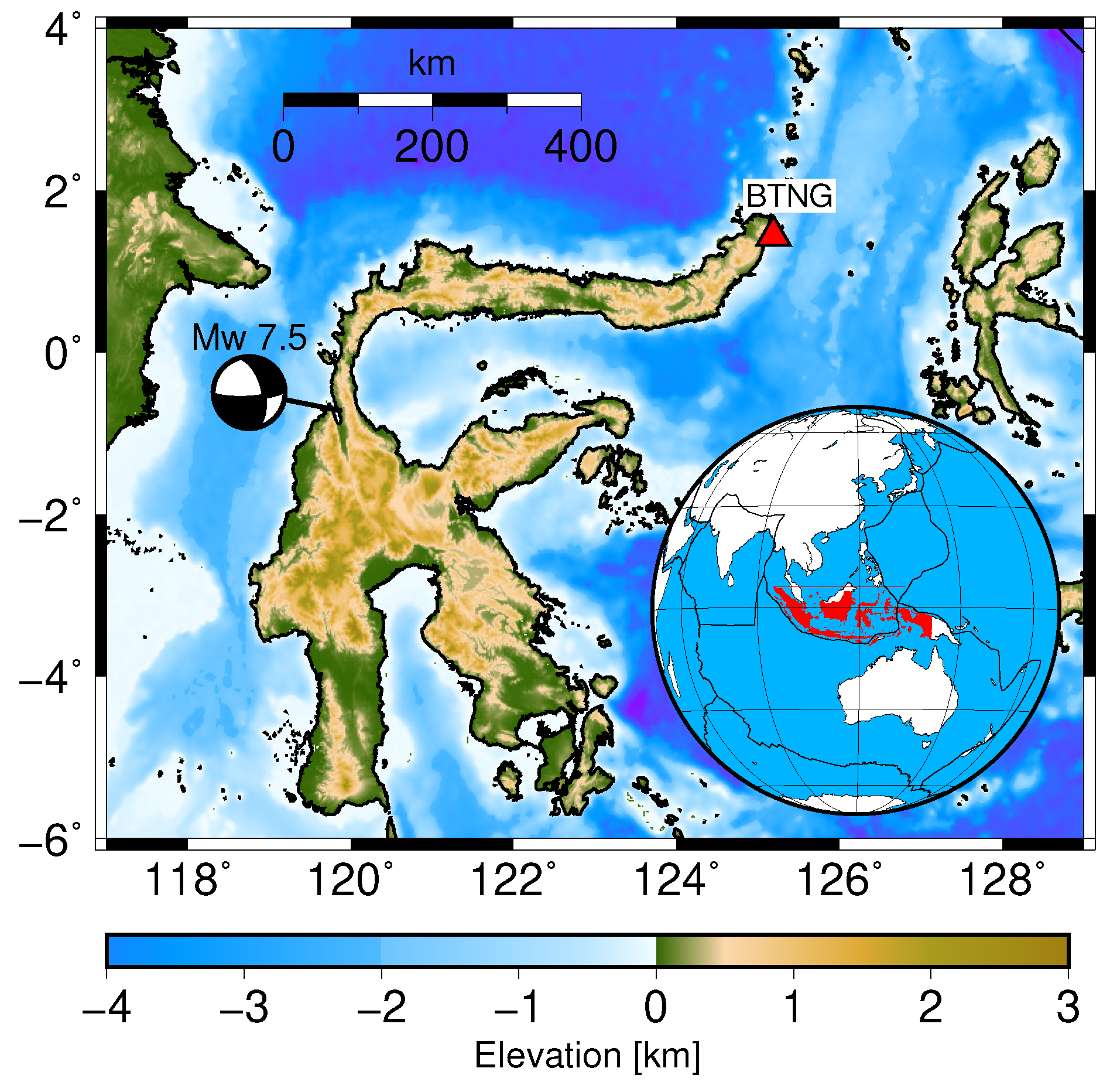
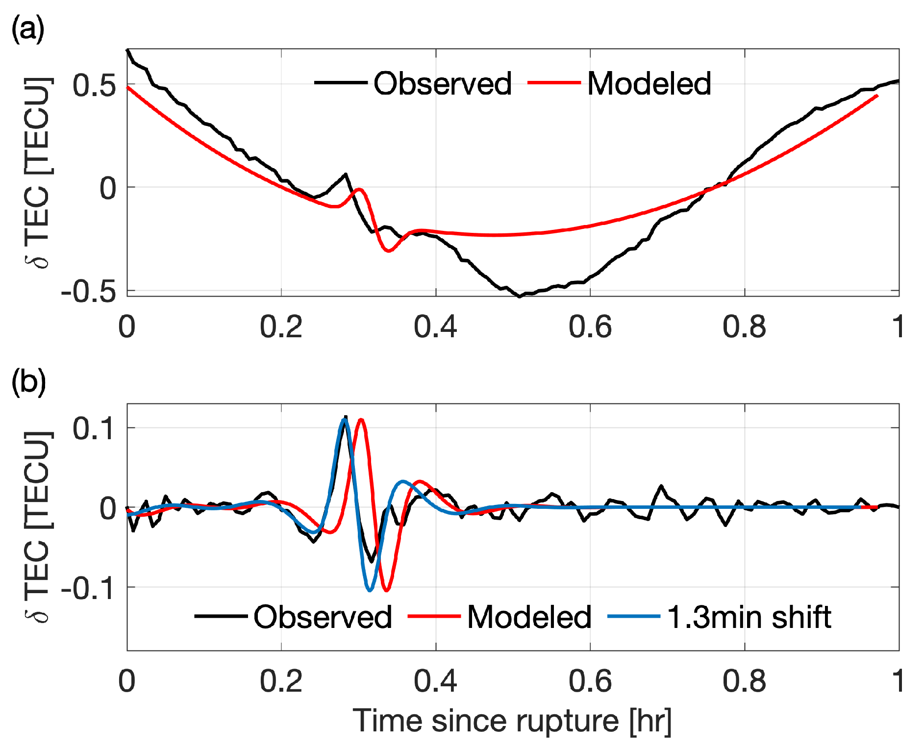
Example: 2018 Sulawesi Earthquakes
4. Discussion
5. Conclusions
Author Contributions
Funding
Acknowledgments
Conflicts of Interest
Abbreviations
| GNSS | global navigation space system |
| IGRF | International Geomagnetic Reference Field |
| IRI | International Reference Ionosphere |
| TEC | total electron content |
| sTEC | slant TEC |
| vTEC | vertical TEC |
| TID | traveling ionospheric disturbance |
| CID | coseismic ionospheric disturbance |
| LOS | line-of-sight |
| CIP | coseismic ionosphere perturbation |
| 2D | two-dimensional |
| 3D | three-dimensional |
| STF | source-time function |
Appendix A. Line-of-Sight Integration
- the receiver location (stationary or non-stationary, e.g., a ground receiver or ship, respectively);
- the satellite location (non-stationary); and
- the electron density along the path (i.e., the line-of-sight or LOS).
- ultra-rapid orbits: released at regular intervals four times per day, which includes both observed and predicted orbits;
- rapid orbits: released approximately 17 h after the end of the previous UTC day; and
- final orbits: released on a weekly basis, approximately 13 days after the end of the solution week.
Appendix B. Divergence in Spherical Coordinates
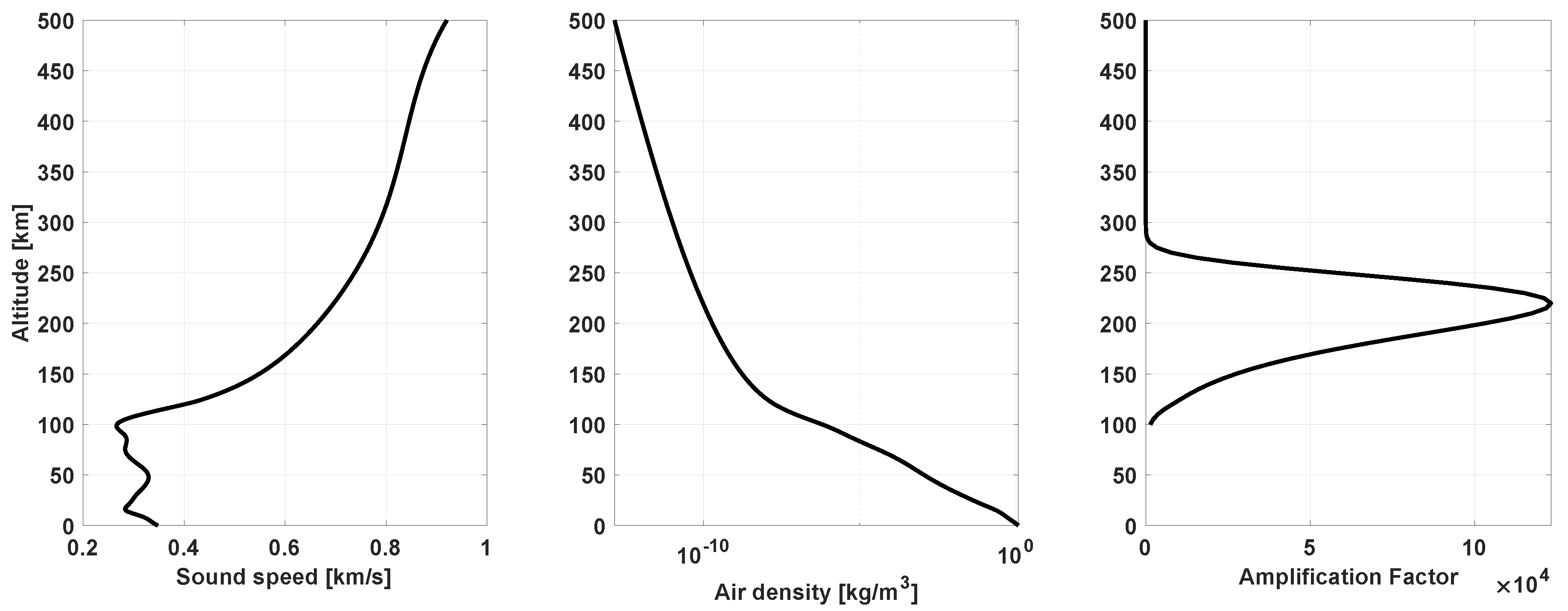
Appendix C. Atmosphere Model
Absorption
References
- United Nations. Factsheet: People and Oceans; The Ocean Conference; United Nations: New York, NY, USA, 5–9 June 2017. [Google Scholar]
- Rolland, L.M.; Occhipinti, G.; Lognonné, P.; Loevenbruck, A. Ionospheric gravity waves detected offshore Hawaii after tsunamis. Geophys. Res. Lett. 2010, 37. [Google Scholar] [CrossRef] [Green Version]
- Beer, T. Atmospheric Waves; Halsted Press Book; Wiley: Hoboken, NJ, USA, 1974. [Google Scholar]
- Schunk, R.; Nagy, A. Ionospheres: Physics, Plasma Physics, and Chemistry; Cambridge Atmospheric and Space Science Series; Cambridge University Press: Cambridge, UK, 2009. [Google Scholar]
- Vadas, S.L.; Crowley, G. Sources of the traveling ionospheric disturbances observed by the ionospheric TIDDBIT sounder near Wallops Island on 30 October 2007. J. Geophys. Res. Space Phys. 2010, 115, 1–24. [Google Scholar] [CrossRef]
- Georges, T.M. Evidence for the influence of atmospheric waves on ionospheric motions. J. Geophys. Res. 1967, 72, 422. [Google Scholar] [CrossRef]
- Hooke, W. Ionospheric irregularities produced by internal atmospheric gravity waves. J. Atmos. Terr. Phys. 1968, 30, 795–823. [Google Scholar] [CrossRef]
- Hooke, W.H. E-region ionospheric irregularities produced by internal atmospheric gravity waves. Planet. Space Sci. 1969, 17, 749–765. [Google Scholar] [CrossRef]
- Georges, T.M.; Hooke, W.H. Wave-induced fluctuations in ionospheric electron content: A model indicating some observational biases. J. Geophys. Res. 1970, 75, 6295–6308. [Google Scholar] [CrossRef]
- Hooke, W.H. Ionospheric response to internal gravity waves: 3. Changes in the densities of the different ion species. J. Geophys. Res. 1970, 75, 7239–7243. [Google Scholar] [CrossRef]
- Hooke, W.H. Ionospheric response to internal gravity waves: 2. Lower F region response. J. Geophys. Res. 1970, 75, 7229–7238. [Google Scholar] [CrossRef]
- Hooke, W.H. The ionospheric response to internal gravity waves: 1. The F2 region response. J. Geophys. Res. 1970, 75, 5535–5544. [Google Scholar] [CrossRef]
- Pilipenko, V.; Belakhovsky, V.; Murr, D.; Fedorov, E.; Engebretson, M. Modulation of total electron content by ULF Pc5 waves. J. Geophys. Res. Space Phys. 2014, 119, 4358–4369. [Google Scholar] [CrossRef]
- Calais, E.; Minster, J.B. GPS detection of ionospheric perturbations following the January 17, 1994, northridge earthquake. Geophyis. Res. Lett. 1995, 22, 1045–1048. [Google Scholar] [CrossRef]
- Bevis, M.; Businger, S.; Herring, T.A.; Rocken, C.; Anthes, R.A.; Ware, R.H. GPS meteorology: Remote sensing of atmospheric water vapor using the global positioning system. J. Geophys. Res. 1992, 97, 15787. [Google Scholar] [CrossRef]
- Houlié, N.; Briole, P.; Nercessian, A.; Murakami, M. Volcanic Plume Above Mount St. Helens Detected with GPS. EOS Trans. 2005, 86, 277–281. [Google Scholar] [CrossRef]
- Pinto Jayawardena, T.S.; Chartier, A.T.; Spencer, P.; Mitchell, C.N. Imaging the topside ionosphere and plasmasphere with ionospheric tomography using COSMIC GPS TEC. J. Geophys. Res. Space Phys. 2016, 121, 817–831. [Google Scholar] [CrossRef]
- Dautermann, T.; Calais, E.; Mattioli, G.S. Global Positioning System detection and energy estimation of the ionospheric wave caused by the 13 July 2003 explosion of the Soufrière Hills Volcano, Montserrat. J. Geophys. Res. 2009, 114, B02202. [Google Scholar] [CrossRef]
- Heki, K.; Ping, J. Directivity and apparent velocity of the coseismic ionospheric disturbances observed with a dense GPS array. Earth Planet. Sci. Lett. 2005, 236, 845–855. [Google Scholar] [CrossRef] [Green Version]
- Heki, K.; Otsuka, Y.; Choosakul, N.; Hemmakorn, N.; Komolmis, T.; Maruyama, T. Detection of ruptures of Andaman fault segments in the 2004 great Sumatra earthquake with coseismic ionospheric disturbances. J. Geophys. Res. 2006, 111, B09313. [Google Scholar] [CrossRef]
- Astafyeva, E.; Rolland, L.M.; Sladen, A. Strike-slip earthquakes can also be detected in the ionosphere. Earth Planet. Sci. Lett. 2014, 405, 180–193. [Google Scholar] [CrossRef]
- Artru, J.; Ducic, V.; Kanamori, H.; Lognonné, P.; Murakami, M. Ionospheric detection of gravity waves induced by tsunamis. Geophys. J. Int. 2005, 160, 840–848. [Google Scholar] [CrossRef] [Green Version]
- Afraimovich, E.L.; Astafyeva, E.I.; Demyanov, V.V.; Edemskiy, I.K.; Gavrilyuk, N.S.; Ishin, A.B.; Kosogorov, E.A.; Leonovich, L.A.; Lesyuta, O.S.; Palamartchouk, K.S.; et al. A review of GPS/GLONASS studies of the ionospheric response to natural and anthropogenic processes and phenomena. J. Space Weather Space Clim. 2013, 3, A27. [Google Scholar] [CrossRef] [Green Version]
- Jin, Y.; Zhou, X.; Moen, J.I.; Hairston, M. The auroral ionosphere TEC response to an interplanetary shock. Geophys. Res. Lett. 2016, 43, 1810–1818. [Google Scholar] [CrossRef] [Green Version]
- Calais, E.; Bernard Minster, J.; Hofton, M.; Hedlin, M. Ionospheric signature of surface mine blasts from Global Positioning System measurements. Geophys. J. Int. 1998, 132, 191–202. [Google Scholar] [CrossRef]
- Bowling, T.; Calais, E.; Haase, J.S. Detection and modelling of the ionospheric perturbation caused by a Space Shuttle launch using a network of ground-based Global Positioning System stations. Geophys. J. Int. 2013, 192, 1324–1331. [Google Scholar] [CrossRef] [Green Version]
- Pichon, A.L.; Blanc, E.; Hauchecorne, A. Infrasound Monitoring for Atmospheric Studies; Springer: Berlin, Germany, 2010. [Google Scholar]
- Rakoto, V.; Lognonné, P.; Rolland, L. Tsunami modeling with solid Earth–ocean–atmosphere coupled normal modes. Geophys. J. Int. 2017, 211, 1119–1138. [Google Scholar] [CrossRef]
- Rakoto, V.; Lognonné, P.; Rolland, L.; Coïsson, P. Tsunami Wave Height Estimation from GPS-Derived Ionospheric Data. J. Geophys. Res. Sp. Phys. 2018, 123, 4329–4348. [Google Scholar] [CrossRef]
- Afraimovich, E.L.; Perevalova, N.P.; Plotnikov, A.V.; Uralov, A.M. The shock-acoustic waves generated by earthquakes. Ann. Geophys. 2001, 19, 395–409. [Google Scholar] [CrossRef] [Green Version]
- Rolland, L.M.; Vergnolle, M.; Nocquet, J.M.; Sladen, A.; Dessa, J.X.; Tavakoli, F.; Nankali, H.R.; Cappa, F. Discriminating the tectonic and non-tectonic contributions in the ionospheric signature of the 2011, M w 7.1, dip-slip Van earthquake, Eastern Turkey. Geophys. Res. Lett. 2013, 40, 2518–2522. [Google Scholar] [CrossRef]
- Cahyadi, M.N.; Heki, K. Coseismic ionospheric disturbance of the large strike-slip earthquakes in North Sumatra in 2012: Mw dependence of the disturbance amplitudes. Geophys. J. Int. 2014, 200, 116–129. [Google Scholar] [CrossRef]
- Rolland, L.M.; Lognonné, P.; Munekane, H. Detection and modeling of Rayleigh wave induced patterns in the ionosphere. J. Geophys. Res. Space Phys. 2011, 116, A05320. [Google Scholar] [CrossRef]
- Occhipinti, G.; Rolland, L.; Lognonné, P.; Watada, S. From Sumatra 2004 to Tohoku-Oki 2011: The systematic GPS detection of the ionospheric signature induced by tsunamigenic earthquakes. J. Geophys. Res. Space Phys. 2013, 118, 3626–3636. [Google Scholar] [CrossRef]
- Lee, R.F.; Rolland, L.M.; Mikesell, T.D. Seismo-Ionospheric Observations, Modeling, and Backprojection of the 2016 Kaikōura Earthquake. Bull. Seismol. Soc. Am. 2018, 108, 1794–1806. [Google Scholar] [CrossRef]
- Thomas, D.; Bagiya, M.S.; Sunil, P.S.; Rolland, L.; Sunil, A.S.; Mikesell, T.D.; Nayak, S.; Mangalampalli, S.; Ramesh, D.S. Revelation of early detection of co-seismic ionospheric perturbations in GPS-TEC from realistic modelling approach: Case study. Sci. Rep. 2018, 8, 12105. [Google Scholar] [CrossRef]
- Poole, A.; Sutcliffe, P. Mechanisms for observed total electron content pulsations at mid latitudes. J. Atmos. Terr. Phys. 1987, 49, 231–236. [Google Scholar] [CrossRef]
- Heki, K. Ionospheric disturbances related to earthquakes. In Advances In Ionospheric Research: Current Understanding and Challenges; Huang, C., Ed.; Wiley/AGU Book: Hoboken, NJ, USA, 2019; Chapter 5-3. [Google Scholar]
- Mannucci, A.J.; Wilson, B.D.; Yuan, D.N.; Ho, C.H.; Lindqwister, U.J.; Runge, T.F. A global mapping technique for GPS-derived ionospheric total electron content measurements. Radio Sci. 1998, 33, 565–582. [Google Scholar] [CrossRef]
- Garner, T.; Gaussiran, T., II; Tolman, B.; Harris, R.; Calfas, R.; Gallagher, H. Total electron content measurements in ionospheric physics. Adv. Space Res. 2008, 42, 720–726. [Google Scholar] [CrossRef]
- Bristow, K.L.; Campbell, G.S. On the relationship between incoming solar radiation and daily maximum and minimum temperature. Agric. For. Meteorol. 1984, 31, 159–166. [Google Scholar] [CrossRef]
- Bilitza, D.; Altadill, D.; Truhlik, V.; Shubin, V.; Galkin, I.; Reinisch, B.; Huang, X. International Reference Ionosphere 2016: From ionospheric climate to real-time weather predictions. Space Weather 2017, 15, 418–429. [Google Scholar] [CrossRef]
- Macleod, M.A. Sporadic E Theory. I. Collision-Geomagnetic Equilibrium. J. Atmos. Sci. 1966, 23, 96–109. [Google Scholar] [CrossRef] [Green Version]
- Lee, R.F. Characterizing Coseismic Ionospheric Disturbance for Surface-Rupturing Earthquakes. Master’s Thesis, Boise State University, Boise, ID, USA, 2017. [Google Scholar]
- Gõmez, D.; Smalley, R.; Langston, C.A.; Wilson, T.J.; Bevis, M.; Dalziel, I.W.D.; Kendrick, E.C.; Konfal, S.A.; Willis, M.J.; Piñõn, D.A.; et al. Virtual array beamforming of GPS TEC observations of coseismic ionospheric disturbances near the Geomagnetic South Pole triggered by teleseismic megathrusts. J. Geophys. Res. A Sp. Phys. 2015, 120, 9087–9101. [Google Scholar] [CrossRef] [Green Version]
- Thébault, E.; Finlay, C.C.; Beggan, C.D.; Alken, P.; Aubert, J.; Barrois, O.; Bertrand, F.; Bondar, T.; Boness, A.; Brocco, L.; et al. International Geomagnetic Reference Field: The 12th generation. Earth Planets Space 2015, 67, 79. [Google Scholar] [CrossRef]
- Kherani, E.A.; Lognonné, P.; Hébert, H.; Rolland, L.; Astafyeva, E.; Occhipinti, G.; Coïsson, P.; Walwer, D.; de Paula, E.R. Modelling of the total electronic content and magnetic field anomalies generated by the 2011 Tohoku-Oki tsunami and associated acoustic-gravity waves. Geophys. J. Int. 2012, 191. [Google Scholar] [CrossRef] [Green Version]
- Zettergren, M.D.; Snively, J.B. Ionospheric response to infrasonic-acoustic waves generated by natural hazard events. J. Geophys. Res. Space Phys. 2015, 120, 8002–8024. [Google Scholar] [CrossRef]
- Zettergren, M.D.; Snively, J.B.; Komjathy, A.; Verkhoglyadova, O.P. Nonlinear ionospheric responses to large-amplitude infrasonic-acoustic waves generated by undersea earthquakes. J. Geophys. Res. Space Phys. 2017, 122, 2272–2291. [Google Scholar] [CrossRef]
- Meng, X.; Verkhoglyadova, O.P.; Komjathy, A.; Savastano, G.; Mannucci, A.J. Physics-Based Modeling of Earthquake-Induced Ionospheric Disturbances. J. Geophys. Res. Space Phys. 2018, 123, 8021–8038. [Google Scholar] [CrossRef]
- Dessa, J.X.; Virieux, J.; Lambotte, S. Infrasound modeling in a spherical heterogeneous atmosphere. Geophys. Res. Lett. 2005, 32, L12808. [Google Scholar] [CrossRef]
- Matoza, R.S.; Fee, D.; Green, D.N.; Le Pichon, A.; Vergoz, J.; Haney, M.M.; Mikesell, T.D.; Franco, L.; Valderrama, O.A.; Kelley, M.R.; et al. Local, Regional, and Remote Seismo-acoustic Observations of the April 2015 VEI 4 Eruption of Calbuco Volcano, Chile. J. Geophys. Res. Solid Earth 2018, 123, 3814–3827. [Google Scholar] [CrossRef]
- Garcia, R.; Lognonné, P.; Bonnin, X. Detecting atmospheric perturbations produced by Venus quakes. Geophys. Res. Lett. 2005, 32, 1–4. [Google Scholar] [CrossRef]
- Lognonné, P.; Clévédé, E.; Kanamori, H. Computation of seismograms and atmospheric oscillations by normal-mode summation for a spherical earth model with realistic atmosphere. Geophys. J. Int. 1998, 135, 388–406. [Google Scholar] [CrossRef] [Green Version]
- Song, X.; Zhang, Y.; Shan, X.; Liu, Y.; Gong, W.; Qu, C. Geodetic Observations of the 2018 Mw 7.5 Sulawesi Earthquake and Its Implications for the Kinematics of the Palu Fault. Geophys. Res. Lett. 2019, 4212–4220. [Google Scholar] [CrossRef]
- Bao, H.; Ampuero, J.P.; Meng, L.; Fielding, E.J.; Liang, C.; Milliner, C.W.; Feng, T.; Huang, H. Early and persistent supershear rupture of the 2018 magnitude 7.5 Palu earthquake. Nat. Geosci. 2019, 12. [Google Scholar] [CrossRef]
- Oppenheim, A.V.; Schafer, R.W.; Buck, J.R. Discrete-Time Signal Processing, 2nd ed.; Prentice Hall: Upper Saddle River, NJ, USA, 1999. [Google Scholar]
- Bagiya, M.S.; Sunil, P.S.; Sunil, A.S.; Ramesh, D.S. Coseismic Contortion and Coupled Nocturnal Ionospheric Perturbations During 2016 Kaikoura, Mw 7.8 New Zealand Earthquake. J. Geophys. Res. Space Phys. 2018, 123, 1–11. [Google Scholar] [CrossRef]
- Picone, J.M.; Hedin, A.E.; Drob, D.P.; Aikin, A.C. NRLMSISE-00 empirical model of the atmosphere: Statistical comparisons and scientific issues. J. Geophys. Res. Space Phys. 2002, 107. [Google Scholar] [CrossRef]
- Tapping, K.F. The 10.7 cm solar radio flux ( F 10.7 ). Space Weather 2013, 11, 394–406. [Google Scholar] [CrossRef]
- Drob, D.P.; Emmert, J.T.; Meriwether, J.W.; Makela, J.J.; Doornbos, E.; Conde, M.; Hernandez, G.; Noto, J.; Zawdie, K.A.; McDonald, S.E.; et al. An update to the Horizontal Wind Model (HWM): The quiet time thermosphere. Earth Space Sci. 2015, 2, 301–319. [Google Scholar] [CrossRef]
- Bass, H.; Sutherland, L.; Piercy, J.; Evans, L. Absorption of sound by the atmosphere. In Physical Acoustics: Principles and Methods. Volume 17 (A85-28596 12-71); Academic Press, Inc.: Orlando, FL, USA, 1984; Volume 17, pp. 145–232. [Google Scholar]
- Bass, H.E.; Chambers, J.P. Absorption of sound in the Martian atmosphere. J. Acoust. Soc. Am. 2001, 109, 3069–3071. [Google Scholar] [CrossRef]
- Landau, L.; Lifshitz, E. Fluid Mechanics: Landau and Lifshitz: Course of Theoretical Physics; Elsevier Science: Amsterdam, The Netherlands, 2013. [Google Scholar]


© 2019 by the authors. Licensee MDPI, Basel, Switzerland. This article is an open access article distributed under the terms and conditions of the Creative Commons Attribution (CC BY) license (http://creativecommons.org/licenses/by/4.0/).
Share and Cite
Mikesell, T.D.; Rolland, L.M.; Lee, R.F.; Zedek, F.; Coïsson, P.; Dessa, J.-X. IonoSeis: A Package to Model Coseismic Ionospheric Disturbances. Atmosphere 2019, 10, 443. https://doi.org/10.3390/atmos10080443
Mikesell TD, Rolland LM, Lee RF, Zedek F, Coïsson P, Dessa J-X. IonoSeis: A Package to Model Coseismic Ionospheric Disturbances. Atmosphere. 2019; 10(8):443. https://doi.org/10.3390/atmos10080443
Chicago/Turabian StyleMikesell, Thomas Dylan, Lucie M. Rolland, Rebekah F. Lee, Florian Zedek, Pierdavide Coïsson, and Jean-Xavier Dessa. 2019. "IonoSeis: A Package to Model Coseismic Ionospheric Disturbances" Atmosphere 10, no. 8: 443. https://doi.org/10.3390/atmos10080443