Observations of Thermally-Driven Winds in a Small Valley during the 21 August 2017 Solar Eclipse

Abstract

On the afternoon of 21 August 2017, a partial solar eclipse occurred over the Blue Ridge Mountains in central Virginia, USA. High-resolution meteorological observations were made on the floor of a small valley to investigate the effect of eclipse-induced cooling on thermally-driven winds. Measurements taken both at the surface and in the lower atmosphere indicate cooling throughout much of the atmospheric boundary layer. Multiple surface weather stations observed wind rotations that occurred both during and after the eclipse, as wind direction shifted from upvalley to downvalley and back to upvalley. The direction of these rotations (clockwise vs. counterclockwise) varied between stations and was strongly influenced by the proximity of the stations to topographic features in the valley. Doppler lidar observations over the valley floor show a 300 m thick layer of downvalley winds that formed below a deeper layer of upvalley winds. Changes in boundary layer winds and structure during the solar eclipse are similar to changes during the morning and evening transitions. However, the subtle differences in the direction of wind rotations between diurnal- and eclipse-transition periods provided important new insights into the interaction between slope- and valley flows, incoming solar radiation, and topographic features.

1. Introduction

Meteorological observations during solar eclipse events date back to the 19th century, when Birt [1] recorded changes in cloud cover during a partial solar eclipse over the United Kingdom. A comprehensive summary of historical eclipse weather observations is given by Aplin et al. [2], who cite more than 100 articles. Some meteorological variables respond similarly across multiple solar eclipses. For example, temperature near the surface drops during the first half of an eclipse, then begins to rise again shortly after totality. However, the response of near-surface winds has been less consistent across eclipse events.

Clayton [3] was the first to propose that a solar eclipse could affect mesoscale wind patterns. He observed changes in wind patterns and an increase in gustiness during the 28 May 1900 eclipse and attributed these observations to the formation of a “cold-air cyclone”. Bigelow [4] disputed this explanation, claiming that the cooling effect of the moon’s shadow was not sufficient to generate large-scale cyclonic flow. Instead, Bigelow [4] hypothesized that the cooling altered the thermally-driven land–sea circulation near the coastal observation site.

Modeling studies have provided evidence that the effect of a solar eclipse on winds is strongest in regions characterized by spatial surface variability. Simulations of the 11 August 1999 solar eclipse over central Europe [5,6] showed the largest changes in wind speed and direction near the coastlines. Gross and Hense [5] described the modelled wind field as ‘a large scale land–sea circulation modified by orographic influences.’ Modifications to land–sea circulations were also clearly visible in simulations of this eclipse over France [7] (their figure 7).

Anomalies in land–sea circulations during solar eclipses have also been confirmed by observational studies. During several eclipse events [8,9], significant shifts in winds were recorded by weather stations in close proximity to bodies of water. In a more comprehensive study of the land–sea circulation, Bala Subrahamanyam and Anurose [10] collected measurements at the surface and aloft at a coastal site in India during the 15 January 2010 total solar eclipse, which began in the late morning hours at the study site. The sea breeze that developed on the eclipse day was weaker at the surface and was approximately 50% of the vertical thickness compared to a non-eclipse control day. Additionally, the onset of the evening land breeze occurred two hours earlier than on the control day.

These modelling and observational studies indicate that land–sea circulations are susceptible to influence from a solar eclipse. Other circulations that result from surface spatial variability are therefore also expected to be influenced by such events. Thermally-driven orographic winds have not been studied to the same extent as land–sea circulations during solar eclipses. These orographic winds exist at spatial scales from a single slope to an entire mountain range, and are caused by differential heating between the atmosphere over the mountains and over the adjacent plains [11]. The winds form a diurnal pattern with upslope and upvalley winds during the day and downslope and downvalley winds at night. Transition periods occur around the time the surface energy budget reverses sign (typically around sunrise and sunset). The time required for winds to reverse during the transition period depends on the dimensions of the valley [12,13], and also on the spatial scale of the flow [14]. Previous studies have observed slope winds [15] and valley winds [16] to reverse direction on time scales of 10–60 min. Hence, local changes to slope and valley winds are expected over the time span of a partial or total solar eclipse (∼2–3 h).

Previous studies have briefly described modifications to orographic winds as a result of solar eclipses. Fernández et al. [17] attributed wind patterns recorded at several surface weather stations during the 11 July 1991 eclipse to local thermally-driven flows. Vogel et al. [18] simulated the 11 August 1999 eclipse over a small domain centered on southern Germany. They found significant changes in wind speed and direction near the mountainous regions in the domain, with minimal modifications to the wind field over homogeneous terrain. Anderson [19] suggested that rapid changes in thermally-driven orographic winds could be partially responsible for the anecdotal reports of the eclipse wind, a sudden increase in wind speed at totality. Eugster et al. [20] used data from 165 surface weather stations in Switzerland to examine temperature and wind changes during the 20 March 2015 solar eclipse. Even though the eclipse was only partial in Switzerland, the cooling was sufficient to delay or prevent the morning transition to upvalley flows.

While eclipse-induced changes in thermally-driven orographic flows have been observed at the surface, the vertical extent of these changes has not been investigated. Upvalley and downvalley winds typically extend vertically throughout the depth of the valley [14] with large changes in the flow structure around the morning and evening transition times [14,21]. A solar eclipse creates conditions that simulate an evening transition immediately followed by a morning transition, providing an opportunity to study the evolution of the valley boundary layer around the transition times in a quasi-laboratory setting.

On 21 August 2017, a total solar eclipse passed over the continental US from Oregon to South Carolina (see [22] for information about the eclipse, including maps of the path of totality). The goal of the present study is to investigate thermally-driven orographic winds in a small valley during the eclipse. Specifically, we investigated the effect of eclipse-induced cooling (and subsequent warming) on changes in speed and direction of the valley wind at the surface and aloft. To this end, we collected observations both at the surface and in the boundary layer which are presented in this paper. We first provide a description of the site in Section 2, followed by instrumentation details in Section 3. We then present and discuss the observations collected during the 21 August eclipse in Section 4 and Section 5. Finally, we provide a summary and conclusions in Section 6.

2. Site Description

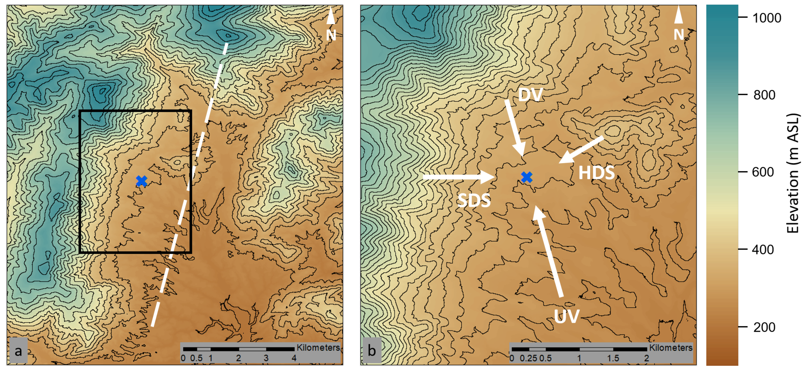
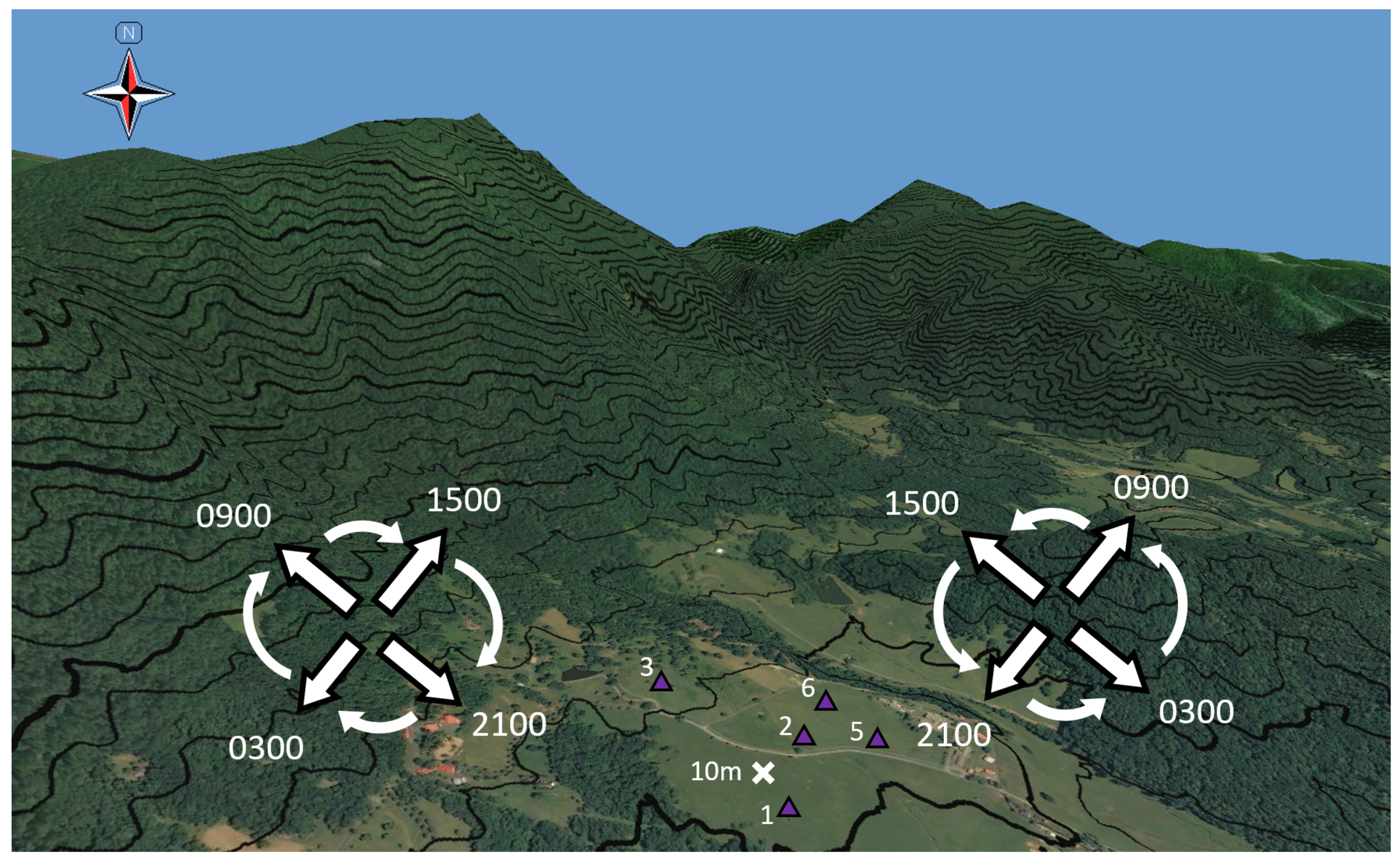
The investigation area is situated on the floor of a small valley in the foothills of the Blue Ridge Mountains, ∼25 km northwest of Charlottesville, Virginia at an altitude of 312 m above mean sea level (ASL). The topography in the valley is complex. On a larger scale, the valley is several kilometers wide and several tens of kilometers long, oriented north to south (Figure 1a). Ridges to the east are ∼700 m ASL, and ridges to the west are ∼850 m ASL. On a smaller scale more local to the investigation area, the north–south oriented valley wind system is deflected by the presence of a small hill reaching ∼100 m above the valley floor (Figure 1b). Hence, the valley wind system is oriented southeast (upvalley) to northwest (downvalley) in the investigation area—see figure 6 in [23]. Previous observations have also revealed that downslope winds can reach the investigation area from both the small hill and the western valley sidewall. In the analysis of wind direction below, hill downslope (HDS) wind refers to downslope wind from the northeast, and sidewall downslope (SDS) wind refers to downslope wind from the west (Figure 1b). Instrumentation was placed in farm fields that were mowed several weeks prior to installation. Vegetation surrounding the towers was predominantly grass at heights ranging from 10–40 cm.

2.1. Eclipse Characteristics

The investigation area was ∼500 km northeast of the path of totality of the 21 August solar eclipse. Eclipse literature separates a total solar eclipse into four phases. First, contact occurs when the moon first moves between the earth and the sun. Second contact refers to the time that totality begins (i.e., the sun is entirely obscured by the moon), and third contact is when totality ends. Fourth (or final, last) contact occurs when the moon no longer obscures the sun. During a partial solar eclipse, only first and final contact occur. A partial eclipse with a maximum solar obscuration of 85.7% occurred over the investigation area. First contact occurred at 13:14 EDT (local time; UTC-04:00), maximum eclipse at 14:41 EDT, and final contact at 16:01 EDT, for a total duration of 2 h 45 min. Local sunrise at the investigation area was 07:01 EDT and local sunset was 18:50 EDT.

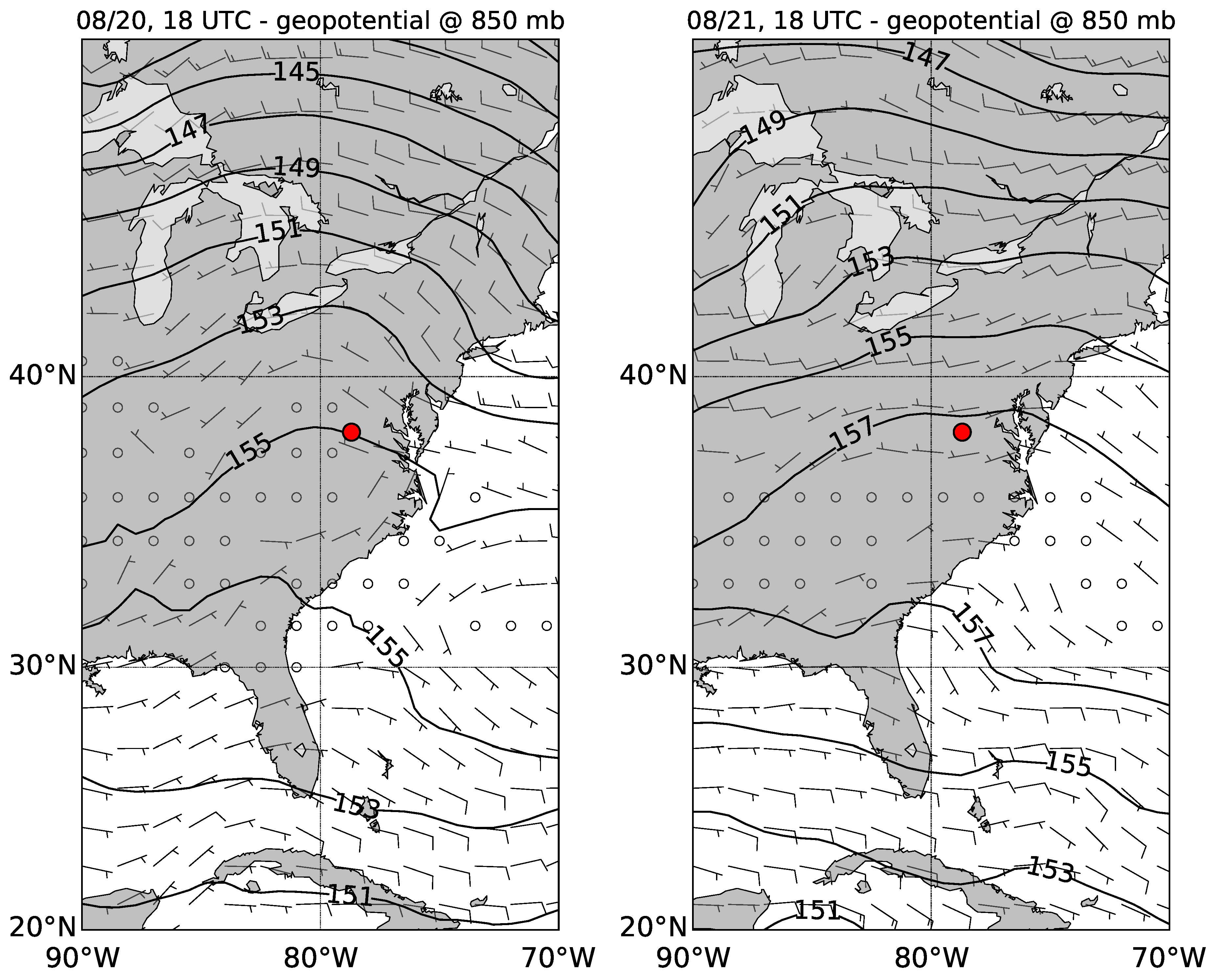
2.2. Synoptic Conditions

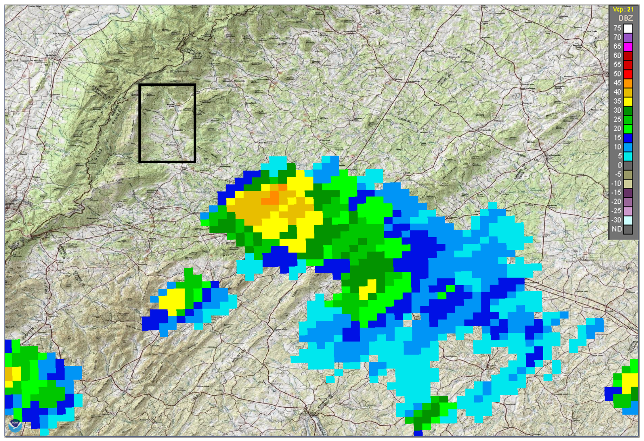
The investigation area was under the influence of high pressure during 20 and 21 August, with westerly winds of about 5 m s${}^{-1}$ at 850 hPa (Figure 2). In the early afternoon hours of 21 August, several small thunderstorm systems were present in the region (Figure 3), with precipitation recorded several kilometers to the south of the investigation area during the eclipse event. The eclipse was not obstructed by thunderstorm clouds at the actual investigation area, and no precipitation was recorded over the area on 21 August. Timelapse photos of cloud cover at the investigation area during the eclipse are provided in the online Supplementary Material.

3. Instrumentation and Data Collection

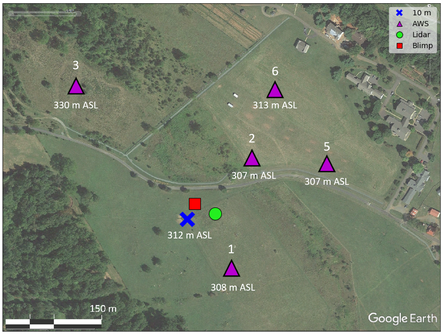
The platforms and instrumentation used in this study included a 10 m meteorological tower, a Doppler lidar, a tethered balloon system (or ‘blimp’), five automated weather stations (AWS), and three radiosondes. Figure 4 shows the layout of instrumentation at the investigation area. Descriptions of each instrument are provided below, with a summary of the details in

Table 1. Instrumentation at the investigation area on 21 August 2017. Abbreviations: temperature (T), relative humidity ($RH$), surface temperature ($T_{skin}$), infrared (IR), shortwave/longwave radiation ($SW$ and $LW$; incoming and outgoing components indicated with up and down arrows, respectively), three-dimensional wind components ($u,\upsilon ,w$), sonic temperature ($T_S$).

	Instrument	Variable	Meas. Height [m AGL]	Samp. Rate [Hz]
Main tower	Apogee ST110 thermistor	T	2.0, 9.4	1.0
	Onset S-THB-M002 thermohygrometer	$RH$	2.0, 9.4	1.0
	Apogee SIF-111 IR radiometer	$T_{skin}$	3.5	0.2
	Apogee SN500 net radiometer	$S{W}^{\downarrow },S{W}^{\uparrow },L{W}^{\downarrow },L{W}^{\uparrow }$	7.0	0.2
	Gill Windmaster 3D sonic anemometer	$u,\upsilon ,w,T_S$	10.0	20
AWS	Decagon DS-2 2D sonic anemometer	$u,\upsilon$	2.3	1.0
	Sensirion SHT15 thermohygrometer	$T,RH$	1.8	0.2
	Bosch BMP180 barometric pressure sensor	P	1.0	1.0
	HALO Photonics StreamLine XR Doppler wind lidar	$WS,WD$	100+	varied
	Kestrel 4500 Weather Tracker (tethered balloon)	$T,RH,P,WS,WD$	0–100	0.5
	Graw DFM-09 radiosonde	$T,RH,P,WS,WD$	0–6000	0.2

.

3.1. Main Tower

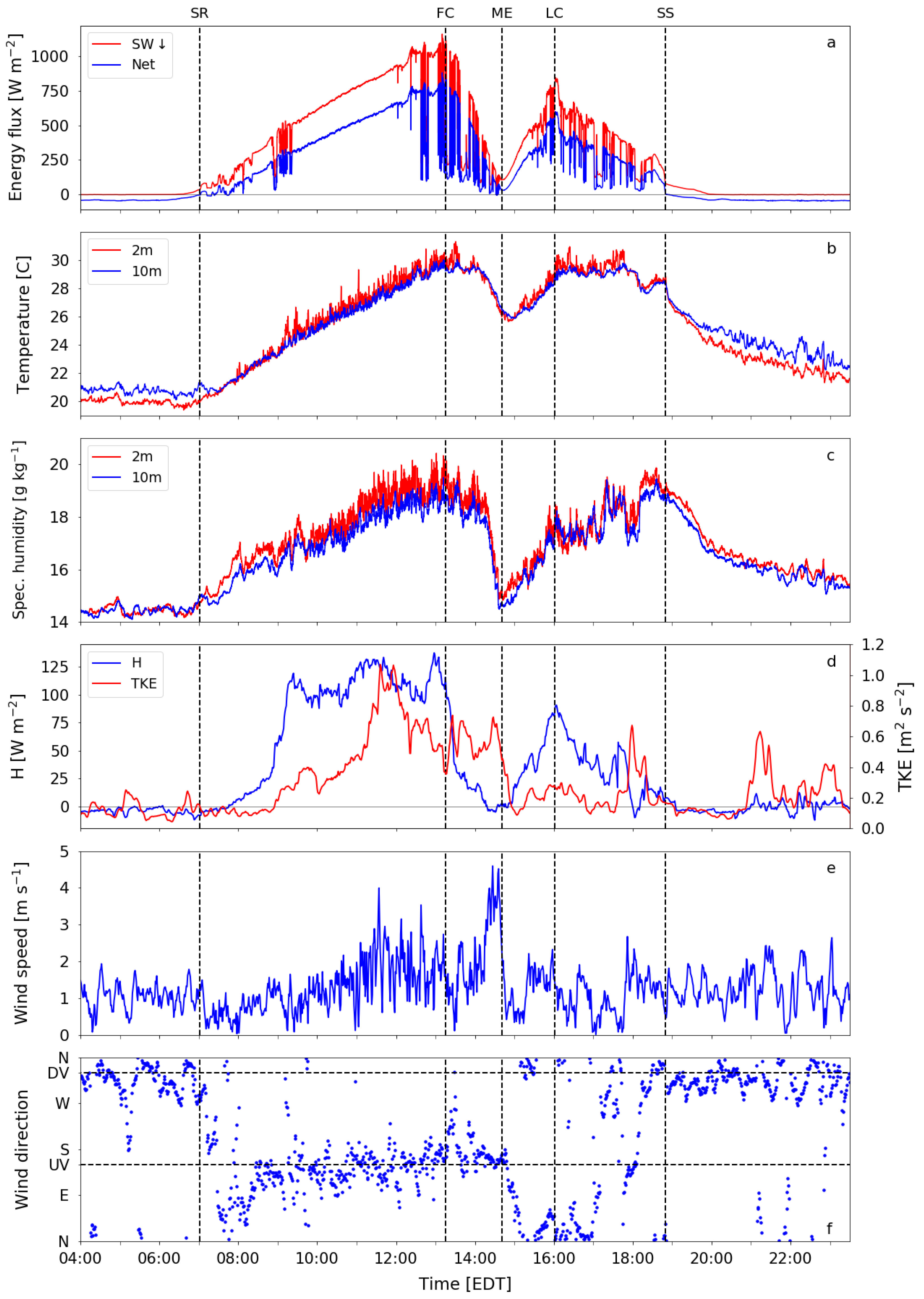
The 10 m main tower is centrally located in the investigation area (Figure 1). The instrumentation includes two shielded, mechanically aspirated thermistors at 2.0 and 9.4 m above ground level (AGL); two shielded, naturally ventilated thermohygrometers at 2.0 and 9.4 m AGL (only humidity observations from these instruments were used for analysis); a four-component net radiometer; a downward-facing infrared radiometer to measure surface temperature mounted at 3.5 m AGL; and a three-dimensional, sonic anemometer at 10 m AGL. The sampling rates for these instruments during the observation period ranged from 0.2 Hz for the net radiometer to 20 Hz for the sonic anemometer (see Table 1). The raw 20 Hz sonic anemometer data are block-averaged to 10 Hz to reduce aliasing effects [24]. Post-processing of the raw sonic anemometer data includes removal of questionable data and associated outliers, rotation of the measured wind speed components into the direction of the mean wind using the double rotation procedure [24,25] and linear detrending to obtain the perturbations of the longitudinal velocity $u^{\prime }$, lateral velocity $v^{\prime }$, vertical velocity $w^{\prime }$ and sonic temperature $T_S^{\prime }$. The sonic anemometer data are also used to calculate sensible heat flux H and turbulent kinetic energy (TKE). For these variables, standard block averages of 30 min do not provide the level of detail necessary to see changes during the eclipse. We present observations of H and TKE every minute, with each observation calculated as a 30-min average that considers the 15 min before and after a given observation.

3.2. AWS

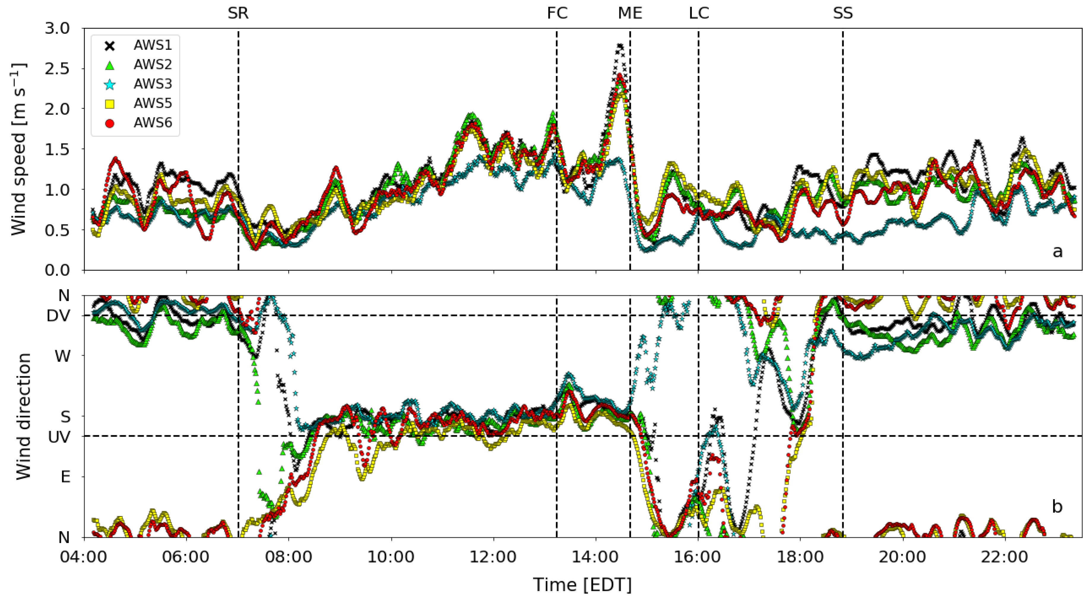
Five Automated Weather Stations (AWS) were deployed at distances ranging from 100 to 300 m from the main tower site to monitor the impact of the solar eclipse on local surface meteorological properties at a high spatial and temporal resolution. These AWS were previously described by van den Bossche and De Wekker [26], and consisted of a 2D sonic anemometer to record wind speed and direction at 1 Hz, and sensors to monitor air temperature and humidity at 0.2 Hz and barometric pressure at 1 Hz, all at a height of 2 m AGL. 1 Hz measurements of wind speed and direction were block-averaged into 1 min periods for analysis.

3.3. Doppler Lidar

To supplement the ground-based observations, we used a scanning Doppler wind lidar (StreamLine XR, Halo Photonics Ltd., Worcestershire, UK), located approximately 20 m east of the main tower (Figure 1b). The lidar was running from 05:39 to 22:30 EDT with only a few gaps due to some power supply issues (from 10:40 to 11:51 EDT and from 17:00 to 17:25 EDT). The lidar was configured to provide vertical profiles of horizontal wind speed and direction every 80 s at a vertical resolution of 29 m, starting at a height of 100 m AGL. We calculated the horizontal wind speed and direction by applying the Velocity Azimuth Display (VAD) algorithm to the radial velocities at each range gate [27]. Similar to Päschke et al. [28], we used n = 12 azimuthal points with an elevation angle of 75 degrees. At each azimuthal point, 30,000 pulsed laser beams of 1.5 μm wavelength were fired, resulting in a dwelling time of approximately 5 s. After each VAD scan pattern, a vertical stare was obtained, which provided vertical wind speed.

3.4. Tethered Balloon Profiles

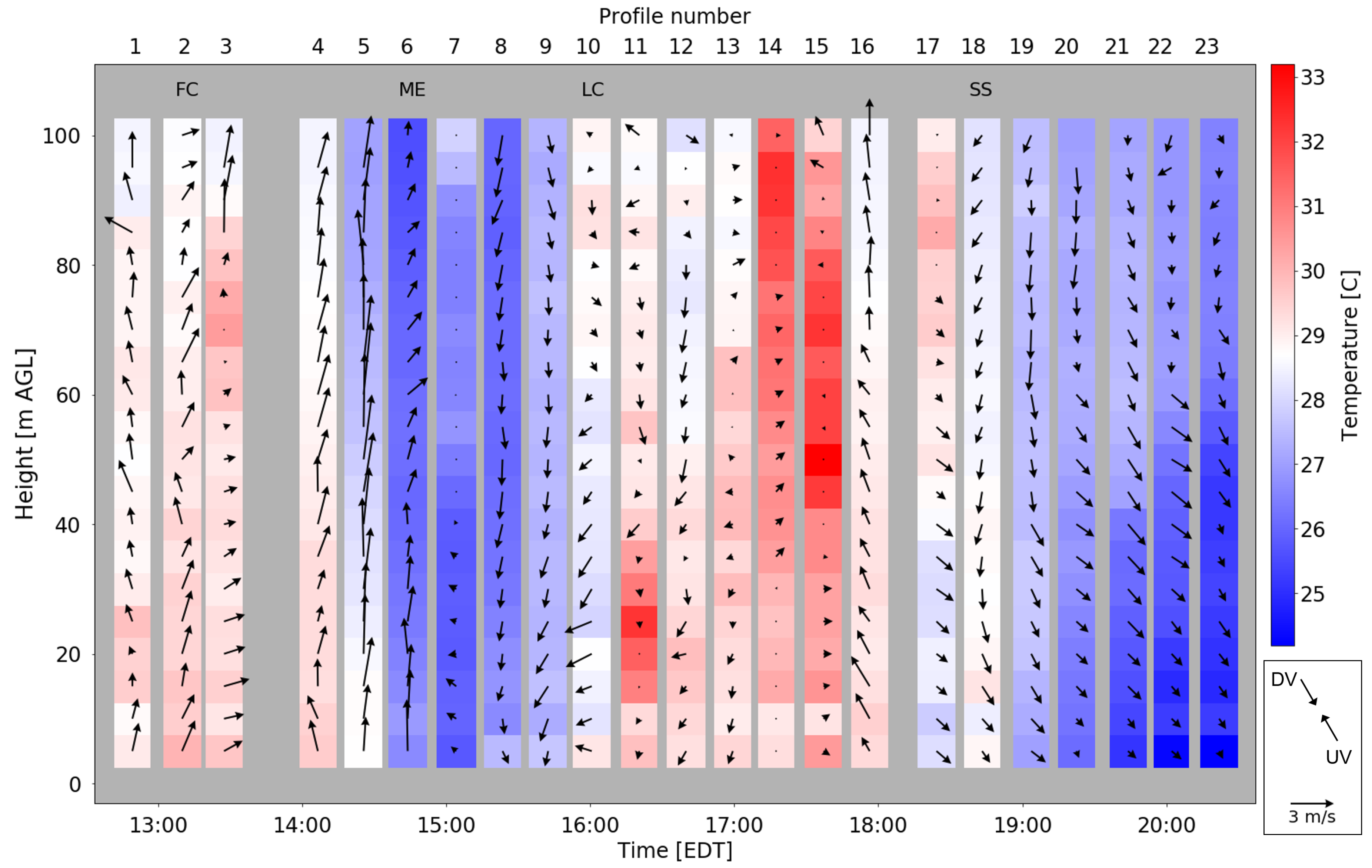
Vertical profiles of temperature, humidity, pressure, and winds from the surface to 100 m AGL were captured using a tethered balloon system during the afternoon and evening hours on 21 August. The system used in this project included a handheld weather meter (Nielsen–Kellerman Kestrel 4500 Pocket Weather Tracker), a wind vane, and a 4 m long helium blimp, similar to the setup used by McKendry et al. [29] and Phelps [30]. Attached to one horizontal end of the cross-shaped wind vane was a large plastic tail which allows the vane to point into the prevailing wind.

To collect the vertical profiles, 100 m of rope was unwound from the winch at a rate of 10 m every 90 s, which allowed the blimp to carry the wind vane and weather meter up from the surface. The sampling rate of the weather meter was 0.5 Hz. Each ascent lasted 15 min, and data collected during the descents were discarded. For analysis, we bin the ascending data by height, with each bin representing the average over 5 m of altitude. During some profiles, the temperature sensor was not well aspirated in the first 5–10 m. Therefore, we exclude the first 10 m of temperature measurements in all profiles from our analysis, and instead use observations from the main tower in the vertical profiles. For each profile, temperature measured at 2 m and 10 m is time-averaged over the duration of the ascent, and these values are used in the first and second bins, respectively.

3.5. Radiosondes

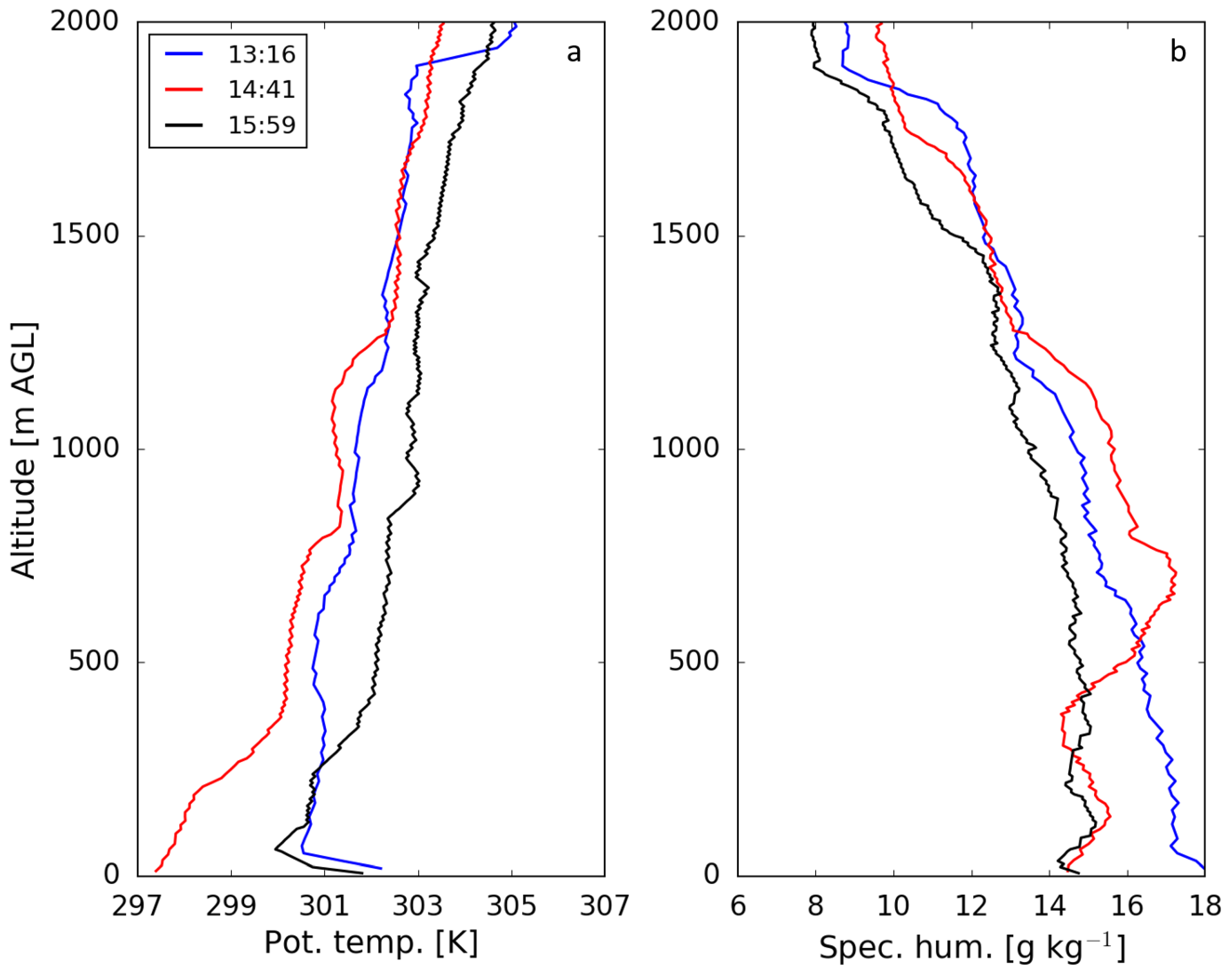
Three Graw DFM-09 radiosondes were launched during the eclipse on 21 August: one close to first contact (actual launch time 13:16 EDT), the second at maximum eclipse (14:41 EDT), and the third close to final contact (15:59 EDT). The radiosondes provided vertical profiles of potential temperature and specific humidity that extend beyond the tethered balloon profiles near the surface. The first two soundings were terminated at an altitude of 5–6 km in order to prepare for subsequent launches. In the following discussion, we focus on the temperature and humidity profiles below 2 km in order to provide finer detail of the atmospheric boundary layer sampled by the lidar.

4. Observations from 13:00–18:00 EDT

4.1. Surface Observations

4.1.1. Surface Temperature and Humidity

First, contact occurred in the early afternoon hours (13:14 EDT) during the presence of a convective boundary layer (CBL). Satellite imagery around this time (not shown) shows convective clouds over much of the southern Appalachian Mountains, an indication of convective instability in the presence of thermally-driven upslope and upvalley flows on a regional scale. Convective cloud cover over the investigation area is apparent in the observations of incoming radiation beginning around 12:00 EDT (Figure 5a). During the eclipse event, incoming shortwave radiation decreased from ∼1000 W m${}^{-2}$ at first contact (13:14 EDT) to a minimum of 105 W m${}^{-2}$ at maximum eclipse (14:41 EDT). Cloud cover over the investigation area persisted throughout the first half of the eclipse, but disappeared at 14:40 EDT. Cloud cover returned again at 15:27 EDT (46 min after maximum eclipse), and persisted throughout the remainder of the afternoon until sunset. Incoming radiation rose to ∼700 W m${}^{-2}$ at final contact. Regional cloud cover showed similar behavior during this period. Hence, a decrease in incoming solar radiation during the eclipse was sufficient to temporarily suppress convection on a regional scale. This effect can be seen on a local scale in the timelapse photos of cloud cover provided in the online Supplementary Material.

An unstable layer existed at the surface in the minutes leading up to first contact, with temperature and specific humidity both decreasing with height at the main tower (Figure 5b,c). A time lag between radiation changes and temperature response is visible in the main tower observations, with temperature decreasing following the decrease in radiation. The vertical temperature gradient at the main tower reversed at 14:06 EDT (35 min before maximum eclipse), indicating the formation of a stable layer at the surface. The timing of this gradient reversal corresponds closely with a change from positive to negative sensible heat flux H (Figure 5d). A sharp drop in specific humidity was observed between 14:15 and 14:40 EDT.

The minimum temperature of 25.6 ${}^{\circ }$C (25.9 ${}^{\circ }$C) at 2 m (10 m) occurred at 14:51 (14:55) EDT, 10 (14) min after maximum eclipse. Temperature at 2 m (10 m) dropped a total of 5.0 ${}^{\circ }$C (3.7 ${}^{\circ }$C) during the eclipse. This decrease is relatively large compared to cooling during other eclipse events. Eugster et al. [20] compiled 130 historical observations of air temperature during solar eclipses dating back to 1834. The majority of these observations were taken within the paths of totality of total solar eclipses. Including the results of the 190 surface weather stations from their study, the average temperature decrease due to a solar eclipse was $1.9\pm 1.4$ ${}^{\circ }$C. The 5.0 ${}^{\circ }$C decrease at 2 m during the partial eclipse at our investigation area is more than two standard deviations larger than average. We note that this average value is based on both partial and total solar eclipse events that occurred at various times throughout the day. Eugster et al. [20] reported that the temperature reduction showed no dependence on eclipse type (partial vs. total), geographic location and several other factors. Additionally, the 5.0 ${}^{\circ }$C recorded decrease is in line with other temperature measurements made across the continental United States by weather stations in the U.S. Climate Reference Network [31].

The vertical temperature gradient at the main tower reversed at 15:00 EDT, 19 min after maximum eclipse. The reversal again corresponded closely to a sign change in H, this time from negative to positive. This reversal indicates that a second CBL formed after maximum eclipse, breaking up the stable boundary layer that formed during the first half.

4.1.2. Surface Winds

Winds at the main tower before first contact were upvalley with speeds around 2 m s${}^{-1}$ (Figure 5e,f). Similar winds were recorded at this time by the five AWS (Figure 6). Winds remained generally upvalley throughout the first half of the eclipse, with a brief rotation towards westerly between 13:20–13:40 EDT recorded at the main tower and four of the five AWS. Wind speeds increased between 14:15–14:40 EDT, with sustained wind speeds at the main tower of 3.5 m s${}^{-1}$ peaking at 4.6 m s${}^{-1}$, the strongest winds recorded throughout the day. The timing of the wind speed increase corresponds with the sharp drop in specific humidity.

Almost immediately after maximum eclipse, winds in the valley changed. At the main tower, the sustained increase in wind speed that began at 14:15 EDT subsided at the exact moment of maximum eclipse, accompanied by a sharp decrease in turbulent kinetic energy (TKE). Winds over the next hour were weak and variable, with 10 m wind speeds peaking below 2 m s${}^{-1}$ and falling below 1 m s${}^{-1}$ in some periods. Southeasterly upvalley winds at 14:41 EDT rotated to north-northeasterly by 15:34 EDT, 27 min before final contact. These north-northeasterly winds persisted until 17:00 EDT (one hour after final contact), then changed to westerly between 17:00 and 17:11 EDT. After a brief period of westerly winds, an abrupt shift back to upvalley winds occurred between 17:44 and 17:49 EDT, accompanied by an increase in wind speed and TKE. Upvalley winds remained until 18:00 EDT. The five AWS also recorded multiple shifts in surface winds in this late afternoon transitional period, ultimately returning to upvalley wind shortly before 18:00 EDT, then rotating quickly to downvalley winds during the evening transition at 18:10 EDT. The timing and direction of the shifts varied between the stations (Figure 6). We examine these wind shifts in more detail in Section 5.

4.2. Boundary Layer Structure and Evolution

Vertical profiles of temperature and wind confirm the presence of an unstable layer at the surface in the minutes leading up to first contact at 13:14 EDT. Profiles collected with the tethered balloon show temperature decreasing with height in the first 100 m AGL, with upvalley winds of 1–3 m s${}^{-1}$ throughout this layer (Figure 7, profile 2). The radiosounding from 13:16 EDT shows an unstable layer at the surface and a capping inversion at approximately 1900 m AGL (Figure 8). Lidar observations show that the layer of upvalley winds visible in the tethered balloon profiles extended to a depth of 400 m AGL at the time of first contact, increasing to 700–800 m AGL at maximum eclipse (Figure 9). Large and fluctuating values of vertical velocity indicate vigorous turbulence in this layer.

After first contact, tethered balloon profiles show a cooling trend throughout the lowest 100 m AGL, with a surface-based stable layer fully established in profile 6 (collected during maximum eclipse). Winds in this layer remained generally upvalley during the first half of the eclipse, and the depth of the upvalley wind layer had extended to the maximum height of the tethered balloon (∼100 m AGL) by maximum eclipse. The radiosonde launched at 14:41 EDT confirms the presence of the stable layer in the tethered balloon profiles, and shows significant cooling during the first half of the eclipse from the surface to approximately 800 m AGL (Figure 8a). Above this developing stable layer was an elevated residual layer of the pre-eclipse CBL. Lidar measurements of vertical wind speed (Figure 9a) still show upward motions above 100 m AGL from 13:14–14:41 EDT that decrease slightly in intensity throughout this period.

The cooling in the atmospheric boundary layer and at the surface during the first half of the eclipse was likely enhanced by factors other than the decrease in solar radiation, including cold air advection associated with the wind speed increase recorded at the main tower between 14:15–14:40 EDT. We hypothesize that the wind speed increase was related to a gust front caused by the downdraft from convective cells 15 km south of the investigation area (Figure 3). The air associated with this gust front, cooled by strong evaporation during the downdraft and channeled by the local topography, undercut the relatively warm and humid air at the investigation area. This caused additional cooling during the eclipse, as well as the sharp drop in specific humidity between 14:15 and 14:40 EDT. The wind speed increase also appears in the lidar data beginning at 14:15 EDT (Figure 9b). Wind speeds of about 4 m s${}^{-1}$ were first observed at the lowest vertical levels (100–150 m AGL). Between 14:40 and 15:00 EDT, this layer of winds lifts off the surface and extends in depth afterwards. This observation corresponds with the conceptual model of a gust front passing over an area [32] (their Figure 3).

During the second half of the eclipse, tethered balloon profiles 7–9 (Figure 8) continue to show a mostly stable boundary layer. Surface warming is visible by profile 10, which began shortly before final contact. By this time, winds in the column had changed from northerly to east-northeasterly. Further aloft, lidar observations show suppressed vertical motion (Figure 9a) and the formation of a downvalley wind layer up to ∼300 m AGL beginning around 15:00 EDT (Figure 9c). Winds in the layer from 300–1000 m AGL began as upvalley during this period, then weakened and changed to westerly synoptic winds.

Warming is apparent throughout the lower atmosphere in the final radiosounding, which was launched at 15:59 EDT. Increasing solar radiation caused near-surface temperatures to almost reach pre-eclipse values. Calculations indicate that heating due to sensible heat flux convergence was not sufficient to account for all the heating that occurred in the boundary layer during this period. Surface weather stations west of the Blue Ridge Mountains (not shown) indicated temperatures that were 1–2 ${}^{\circ }$C warmer than at the investigation area at the time of first contact. During the second half of the eclipse, as the layer of upvalley winds eroded and westerly synoptic winds became the dominant flow above the investigation area (Figure 9c), the relatively warm boundary layer air was transported over the mountains and contributed to the warming of the boundary layer in the investigation area.

After final contact, the second CBL continued to develop at the surface as incoming radiation returned to typical afternoon levels and temperature increased in the CBL (Figure 7, profiles 11–13). Strong vertical motions were again initiated near the surface (Figure 9a), but were not re-established above an altitude of 600 m AGL. Hence, although the increased radiation after 14:41 EDT was enough to break up the surface stable layer that formed during the eclipse, it was not enough for the CBL to attain a depth typical of a warm summer day.

Measurements in the lower atmosphere show that the period of transitional winds after final contact was not limited to the surface. Winds were light with a highly variable direction during profiles 11–15 recorded by the tethered balloon (Figure 7). In profile 16, the final profile of the late afternoon hours, southeasterly upvalley winds were re-established below 60 m AGL. In the lidar observations, a gap in the data exists between 17:00 and 17:40 EDT. When observations came back online at 17:40 EDT, winds above the valley floor had changed back to upvalley up to a height of 400 m AGL.

5. Wind Rotations during Transition Periods

Winds in and above the investigation area changed direction several times during and after the solar eclipse. Winds from the upvalley, downvalley, and downslope directions were all recorded at the main tower and the five AWS during the daytime hours of 21 August. However, significant differences in the timing and magnitude of wind direction changes existed between the various towers. Specifically, we note several periods of changing winds when the rotational direction of the change (i.e., a clockwise or counterclockwise rotation) varied between the towers.

Hawkes [33] was the first to describe the daily rotation of wind direction over valley sidewalls due to the interaction of thermally-driven slope and valley winds. An observer on the valley floor looking toward the head of the valley would see a daily clockwise (CW) rotation over the left sidewall and a counterclockwise (CCW) rotation over the right sidewall (Figure 10). Such rotations have been confirmed in previous observational and modeling studies [12,34,35]. We now use this conceptual model as a framework to explain the wind rotations observed during and after the solar eclipse.

The idealized valley shape in Hawkes’ conceptual model [33] results in a rotational pattern where one sidewall exactly mirrors the other, so that the same component of slope or valley wind exists simultaneously over both sidewalls. During a typical morning transition in our investigation area, the eastern face of the valley sidewall is heated for several hours after sunrise before the southwestern face of the hill receives any direct radiation. Therefore, we expect upslope winds to start over the sidewall before they begin over the hill. During the evening transition, the last rays of the afternoon sun illuminate the southwestern face of the hill. Meanwhile, the valley sidewall to the west has been shaded for some time. We expect that downslope winds will also develop earlier over the sidewall than over the hill. In addition to this temporal offset, the hill and the sidewall do not face each other directly. Downslope winds from the sidewall are westerly, whereas downslope winds from the hill are northeasterly. Hence, daily wind rotations with opposing directions are still expected over the sidewall and hill, but the rotations are not expected to be as symmetrical as those depicted in Hawkes’ model. Looking toward the head of the valley in our investigation area, the conceptual model predicts a CW rotation over the sidewall and a CCW rotation over the hill.

Observations from the main tower and five AWS provide evidence that wind rotations also exist at locations along the valley floor. These rotations occur in different directions (CW vs. CCW) and at different times of day depending on the locations of the towers. The rotational direction at the various locations is influenced by the proximity of the location to the two main topographic features in the investigation area, the sidewall and the hill. Additionally, differences in solar altitude and azimuth angles between the eclipse and the morning and evening transition periods resulted in different wind patterns during those three events. We separate the patterns of wind rotation into three groups: sidewall-influenced, hill-influenced, and hybrid-influenced rotations. In the final category, both topographic features influenced the wind patterns at various points throughout the day.

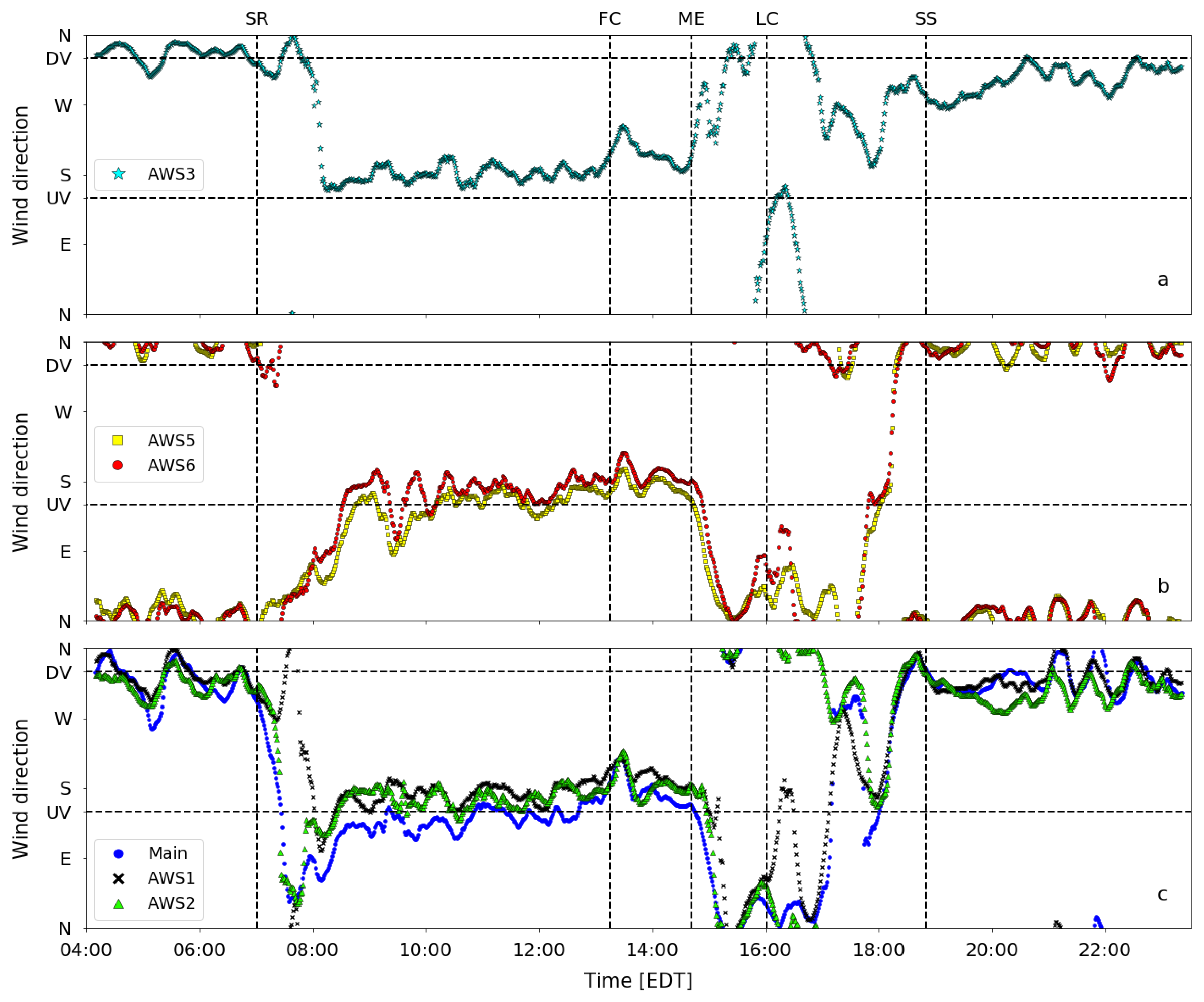
5.1. Sidewall-Influenced Towers: AWS3

AWS3 was the station installed closest to the western sidewall (Figure 1 and Figure 4). Winds before sunrise on 21 August were steadily downvalley (Figure 11). During the morning transition, winds rotated CCW from downvalley to upvalley in less than 10 min. This CCW rotation is in the opposite direction of what is predicted when applying Hawkes’ conceptual model [33] to the topography in the investigation area. We note that AWS3 was installed on the valley floor near the sidewall, and not actually on the slope itself. Therefore, we expect upslope flows over the sidewall to have minimal influence on wind observations made by AWS3. Additionally, wind speeds of less than 1 m s${}^{-1}$ during the morning transition indicate that extremely localized flows, possibly influenced by microterrain features or vegetation, may have affected wind observations during this period.

Upvalley winds established at AWS3 after the morning transition remained until maximum eclipse at 14:41 EDT, then began a CW rotation toward downvalley winds. This rotation occurred in the direction predicted by the conceptual model. The decrease in radiation during the first half of the eclipse caused the atmosphere over the sidewall to cool and southeasterly upvalley winds to change to westerly downslope winds. For more than an hour after final contact, AWS3 continued to observe rotating winds in both the CW and CCW directions. Similarly to the morning transition, wind speeds during this late afternoon period were very low, sometimes falling below 0.5 m s${}^{-1}$. Again, extremely local effects contributed to these anomalous rotations.

Winds at AWS3 briefly returned to upvalley around 17:50 EDT, only a few minutes before the evening transition began. Winds then rotated CW to downvalley, again in less than 10 min. This rotation again aligns with the conceptual model, with a brief influence of sidewall downslope winds before downvalley winds dominate at the station. However, wind speeds recorded during this period and into the nighttime hours were still relatively low at less than 1 m s${}^{-1}$. Downvalley winds persisted at AWS3 throughout the rest of the night.

5.2. Hill-Influenced Towers: AWS5, AWS6

AWS5 and AWS6 were the two stations in closest proximity to the hill (Figure 4). Nighttime winds at these two stations were northeasterly or northerly instead of the expected northwesterly downvalley direction. We suspect that this is a result of north-northeasterly downvalley winds in the larger valley moving over the hill and mixing down into the investigation area (see Figure 1). Shortly after sunrise at 07:01 EDT, winds began a CW rotation toward upvalley winds, which were established around 09:00 EDT. This CW rotation during the morning transition is in the opposite rotational direction of what is predicted when applying Hawkes’ conceptual model [33] to the topography in the investigation area. In theory, southwesterly upslope flows over the hill should rotate CCW and change to southeasterly upvalley flows during the morning transition (Figure 10). However, because our stations were installed on the valley floor near the hill (instead of on the actual slopes of the hill), we expect minimal influence of upslope flows on wind observations at AWS5 and AWS6.

Similarly to observations at AWS3, upvalley winds established at AWS5 and AWS6 after the morning transition remained until maximum eclipse at 14:41 EDT. Shortly afterwards, winds near the two stations began a CCW rotation toward northeasterly winds. This rotation aligns with expectations from the conceptual model. As incoming radiation decreased during the first half of the eclipse, the atmosphere over the hill cooled at the same time as the atmosphere over the sidewall. At AWS5 and AWS6, southeasterly upvalley winds gave way to northeasterly hill downslope winds. However, both stations observed two additional CW wind rotations in the late afternoon hours. The first was a CW rotation from northerly/northeasterly to upvalley winds, similar to the rotation that occurred during the morning transition. This rotation was followed closely by a second CW rotation from upvalley back to northerly/northeasterly winds during the evening transition. This second rotation can be explained by the hill’s aspect. The last rays of the afternoon sun were incident upon the southwestern face of the hill while the valley sidewall to the west had been shaded for some time. Downslope winds developed earlier over the sidewall than over the hill, and these westerly downslope winds were able to reach AWS5 and AWS6 and cause the CW rotation to typical northerly/northeasterly nighttime winds at these stations.

5.3. Hybrid-Influenced Towers: Main Tower, AWS1, AWS2

The main 10 m tower, AWS1, and AWS2 were centrally located on the valley floor (Figure 4) and recorded wind observations influenced by both the hill and the sidewall at different points during the day. All three stations recorded downvalley winds in the early morning hours before sunrise, which rotated CCW during the morning transition. Again, low wind speeds indicate that a strong thermally-driven component was not present during the morning transition. Shortly before 08:00 EDT, the main tower and AWS2 recorded northeasterly wind that gradually rotated CW toward upvalley. This is similar to the pattern recorded by AWS5 and AWS6, the towers in close proximity to the hill. Meanwhile, the initial CCW rotation recorded at AWS1 settled at upvalley winds without a period of northeasterly wind. This pattern is closer to the one recorded by AWS3, the tower nearest the sidewall.

The main tower, AWS1, and AWS2 all recorded CCW rotations from upvalley to northeasterly winds during the second half of the eclipse, aligning closely with the observations recorded by AWS5 and AWS6. This is a result of the relative size of the two main terrain features at the observation site. The atmosphere over the hill cooled more quickly than the atmosphere over the sidewall, resulting in an earlier onset of hill downslope winds from the northeast. Later, the main tower, AWS1, and AWS2 recorded a period of westerly winds between 17:00 and 17:45 EDT. This suggests that sidewall downslope winds from the west became strong enough to overpower the hill downslope winds from the northeast at these stations. However, during this transitional period of low wind speeds, microterrain or vegetation features can complicate the wind patterns.

As at the other stations, winds at the main tower, AWS1, and AWS2 returned to upvalley shortly before 18:00 EDT. The three stations recorded a CW rotation to downvalley winds, providing additional evidence that sidewall downslope winds were strong enough to reach all stations in the observation area. Downvalley winds remained throughout the nighttime hours.

6. Summary, Conclusions, and Future Work

The focus of this study was the observation of boundary layer structure and thermally-driven orographic winds during the 21 August 2017 solar eclipse. We observed these winds in a small valley to determine if eclipse-induced changes in radiation and temperature were sufficient to disrupt the normal diurnal cycle of slope and valley winds. Our analysis of the observations provided the following results:

• Surface cooling was more than two standard deviations larger than average compared to previous solar eclipse events, but was similar to other temperature decreases recorded across the continental U.S. during the 21 August eclipse. This cooling in the presence of negative daytime sensible heat flux caused the formation of a stable layer at the surface.
• Vertical temperature profiles from tethered balloons and radiosondes indicate that cooling during the first half of the eclipse extended to 800 m AGL, and warming during the second half extended above 2000 m AGL. The daytime sensible heat flux was not sufficient to explain the cooling and warming of the lower atmosphere, and temperature advection likely played an important role.
• Surface weather stations recorded multiple rotations in wind direction during and after the eclipse. These rotations can be explained by the interaction between slope and valley flows. The size and direction of the rotations were strongly influenced by the proximity of the stations to local terrain features. Rotations recorded during the eclipse generally aligned with expectations from a conceptual model [33], but rotations during the morning and evening transitions did not always occur in the expected directions. The high solar elevation angle and low azimuth angle during the eclipse caused different slope heating and cooling patterns to develop than what would typically occur during the transition periods.
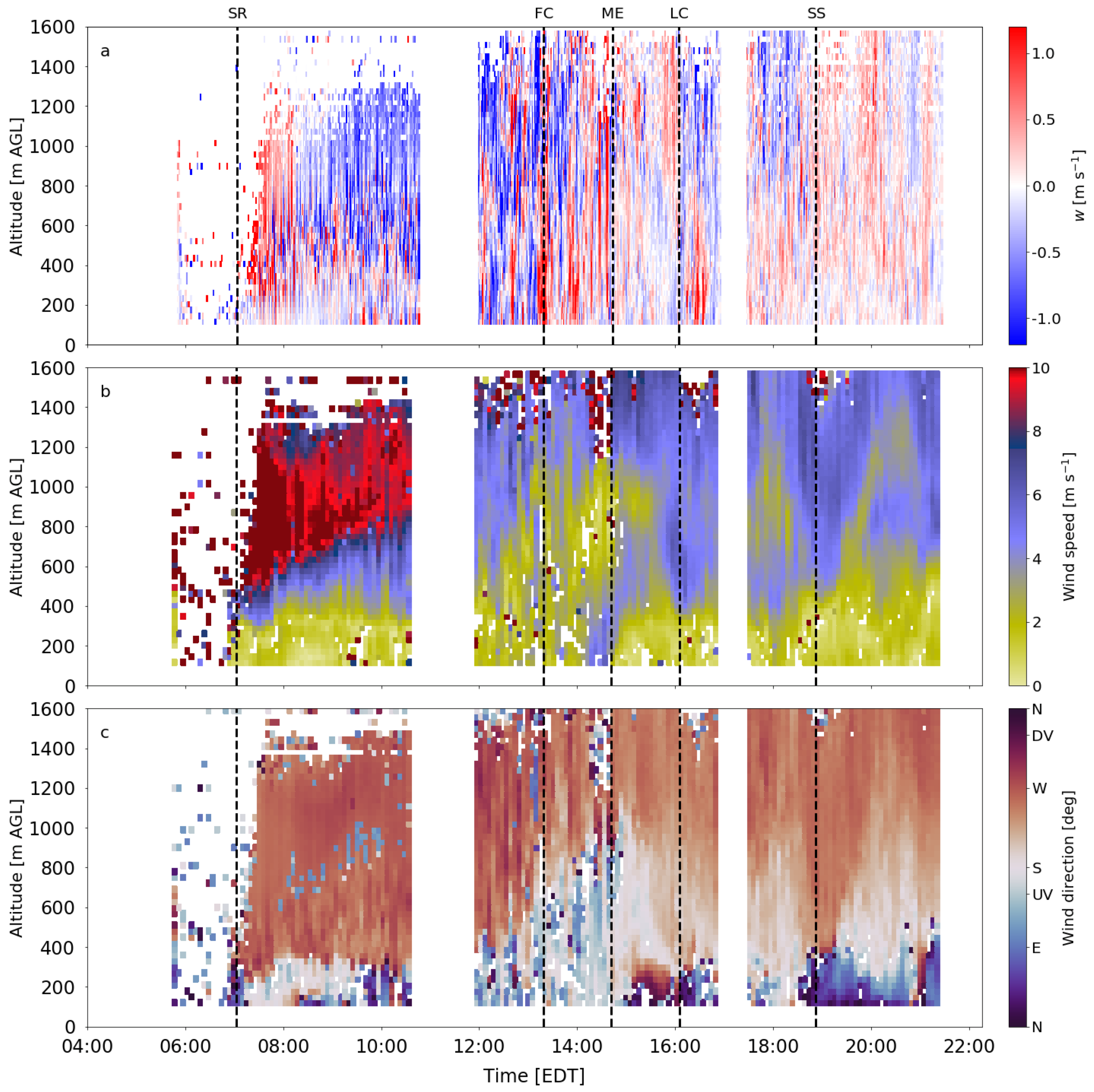
• Tethered balloon and lidar observations showed that wind shifts and rotations were not limited to the surface. A layer of downvalley winds formed between the surface and ∼300 m AGL during the second half of the eclipse. Winds above this layer remained upvalley or westerly. The timing of the appearance of this wind layering relative to the solar eclipse indicates a time lag between decreased radiation during the eclipse and the reversal of the valley wind system. Downvalley wind at the surface was not initiated until ∼80 min after the start of the eclipse. This downvalley wind layer existed for ∼70 min and dissipated shortly after final contact.

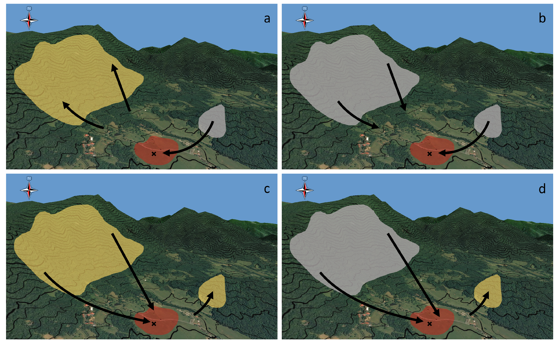
We conclude that the decreased radiation and associated cooling during the solar eclipse altered the expected cycle of thermally-driven winds in the valley. With regard to incoming solar radiation, the first and second halves of the eclipse are similar to the evening and morning transitions, respectively, but with important differences caused by the orientation of the topographic features relative to the position of the sun. A revised conceptual diagram summarizes the interactions between solar radiation, topography, and winds that occurred on 21 August (Figure 12). Incoming solar radiation shortly after sunrise was incident on the east-facing sidewall, resulting in upslope winds over the sidewall while downslope winds persisted over the west-facing hill (Figure 12a). The sidewall and hill experienced simultaneous cooling during the first half of the eclipse, and downslope winds formed first over the hill due to its smaller size relative to the sidewall (Figure 12b). The two topographic features were simultaneously heated during the second half of the eclipse, and upslope winds formed over the hill while downslope winds were still present over the sidewall (Figure 12c). Finally, during the evening transition, downslope winds began over the shaded sidewall while the hill continued to receive late afternoon solar radiation (Figure 12d).

The interaction between the phases of the slope and valley wind systems causes a daily wind direction rotation on the valley sidewalls [11,33]. The observations from 21 August in the present study indicate that the explanation of the nature of rotations over sidewalls can be extended to locations at and above the valley floor. The magnitude and direction of rotation at various locations over the valley floor appear to vary between the morning and evening transitions, and are also dependent on interactions between incoming solar radiation and local terrain features. These rotations can impact e.g., the dispersion of air pollutants from emission sources in different parts of the valley, and therefore can have important implications for air quality studies.

This study focused on the observations collected only on the day of the eclipse. We were fortunate that calm synoptic conditions prevailed at the investigation area on 21 August, and that precipitation from the thunderstorm system south of the site did not disrupt our measurement campaign. Future work will include an analysis of one year of data from the main tower. We will characterize ‘typical’ wind and temperature changes during morning and evening transitions at our site, and interpret the deviation of the wind patterns during the solar eclipse in more detail. We will pay special attention to the climatology of wind rotations on the valley floor.

References

1. Birt, W. Meteorological Observations Made during the Solar Eclipse of May 15, 1836, at Greenwich. Lond. Edinb. Phil. Mag. 1836, 9, 393–394. [Google Scholar]
2. Aplin, K.L.; Scott, C.J.; Gray, S.L. Atmospheric Changes from Solar Eclipses. Phil. Trans. R. Soc. A 2016, 374, 20150217. [Google Scholar] [CrossRef] [PubMed]
3. Clayton, H.H. The Eclipse Cyclone and the Diurnal Cyclones. Ann. Astron. Obs. Harv. Coll. 1901, 43, 5–31. [Google Scholar]
4. Bigelow, F.H. Eclipse Meteorology and Allied Problems; U.S. Department of Agriculture Weather Bureau Bulletin I 267; U.S. Department of Agriculture: Washington, DC, USA, 1902.
5. Gross, P.; Hense, A. Effects of a Total Solar Eclipse on the Mesoscale Atmospheric Circulation over Europe—A Model Experiment. Meteorol. Atmos. Phys. 1999, 71, 229–242. [Google Scholar] [CrossRef]
6. Prenosil, T. The Influence of the 11 August 1999 Total Solar Eclipse on the Weather over Central Europe. Meteorologische Zeitschrift 2000, 9, 351–359. [Google Scholar] [CrossRef]
7. Piriou, J.; Lamboley, P. Prévision Numérique Des Effets Météorologiques d’une Éclipse de Soleil. La Météorologie 1999, 8, 52–56. [Google Scholar] [CrossRef]
8. Founda, D.; Melas, D.; Lykoudis, S.; Lisaridis, I.; Gerasopoulos, E.; Kouvarakis, G.; Petrakis, M.; Zerefos, C. The Effect of the Total Solar Eclipse of 29 March 2006 on Meteorological Variables in Greece. Atmos. Chem. Phys. 2007, 7, 5543–5553. [Google Scholar] [CrossRef]
9. Gray, S.L.; Harrison, R.G. Diagnosing Eclipse-Induced Wind Changes. Proc. R. Soc. A 2012, 468, 1839–1850. [Google Scholar] [CrossRef]
10. Bala Subrahamanyam, D.; Anurose, T.J. Solar Eclipse Induced Impacts on Sea/Land Breeze Circulation over Thumba: A Case Study. J. Atmos. Sol.-Terr. Phys. 2011, 73, 703–708. [Google Scholar] [CrossRef]
11. Whiteman, C.D. Mountain Meteorology: Fundamentals and Applications; Oxford University Press: New York, NY, USA, 2000; p. 355. [Google Scholar]
12. Whiteman, C.D.; Allwine, K.J.; Fritschen, L.J.; Orgill, M.M.; Simpson, J.R. Deep Valley Radiation and Surface Energy Budget Microclimates. Part II: Energy Budget. J. Appl. Meteorol. 1989, 28, 427–437. [Google Scholar] [CrossRef] [Green Version]
13. Pardyjak, E.R.; Fernando, H.J.S.; Hunt, J.C.; Grachev, A.A.; Anderson, J. A Case Study of the Development of Nocturnal Slope Flows in a Wide Open Valley and Associated Air Quality Implications. Meteorologische Zeitschrift 2009, 18, 85–100. [Google Scholar] [CrossRef] [PubMed]
14. Zardi, D.; Whiteman, C.D. Diurnal Mountain Wind Systems. In Mountain Weather Research and Forecasting; Chow, F.K., De Wekker, S.F.J., Snyder, B.J., Eds.; Springer Atmospheric Sciences; Springer: Dordrecht, The Netherlands, 2013; pp. 35–119. [Google Scholar] [CrossRef]
15. Nadeau, D.F.; Pardyjak, E.R.; Higgins, C.W.; Huwald, H.; Parlange, M.B. Flow during the Evening Transition over Steep Alpine Slopes. Q. J. R. Meteorol. Soc. 2013, 139, 607–624. [Google Scholar] [CrossRef]
16. Duine, G.J.; Hedde, T.; Roubin, P.; Durand, P.; Lothon, M.; Lohou, F.; Augustin, P.; Fourmentin, M. Characterization of Valley Flows within Two Confluent Valleys under Stable Conditions: Observations from the KASCADE Field Experiment. Q. J. R. Meteorol. Soc. 2017, 143, 1886–1902. [Google Scholar] [CrossRef]
17. Fernández, W.; Castro, V.; Hildago, H. Air Temperature and Wind Changes in Costa Rica during the Total Solar Eclipse of July 11, 1991. Earth Moon Planets 1993, 63, 133–147. [Google Scholar] [CrossRef]
18. Vogel, B.; Baldauf, M.; Fiedler, F. The Influence of a Solar Eclipse on Temperature and Wind in the Upper-Rhine Valley—A Numerical Case Study. Meteorologische Zeitschrift 2001, 10, 207–214. [Google Scholar] [CrossRef]
19. Anderson, J. Meteorological Changes during a Solar Eclipse. Weather 1999, 54, 207–215. [Google Scholar] [CrossRef]
20. Eugster, W.; Emmel, C.; Wolf, S.; Buchmann, N.; McFadden, J.P.; Whiteman, C.D. Effects of Vernal Equinox Solar Eclipse on Temperature and Wind Direction in Switzerland. Atmos. Chem. Phys. 2017, 17, 14887–14904. [Google Scholar] [CrossRef]
21. Lothon, M.; Lohou, F.; Pino, D.; Couvreux, F.; Pardyjak, E.R.; Reuder, J.; Vilà-Guerau de Arellano, J.; Durand, P.; Hartogensis, O.; Legain, D.; et al. The BLLAST Field Experiment: Boundary-Layer Late Afternoon and Sunset Turbulence. Atmos. Chem. Phys. 2014, 14, 10931–10960. [Google Scholar] [CrossRef]
22. NASA. Total Solar Eclipse—August 21, 2017. 2017. Available online: https://eclipse2017.nasa.gov (accessed on 11 July 2019).
23. Pal, S.; Lee, T.R.; Phelps, S.; De Wekker, S.F.J. Impact of Atmospheric Boundary Layer Depth Variability and Wind Reversal on the Diurnal Variability of Aerosol Concentration at a Valley Site. Sci. Total. Environ. 2014, 496, 424–434. [Google Scholar] [CrossRef]
24. Kaimal, J.C.; Finnigan, J.J. Atmospheric Boundary Layer Flows: Their Structure and Measurement; Oxford University Press: Oxford, UK, 1994. [Google Scholar]
25. Wilczak, J.M.; Oncley, S.P.; Stage, S.A. Sonic anemometer tilt correction algorithms. Bound.-Layer Meteorol. 2001, 99, 127–150. [Google Scholar] [CrossRef]
26. van den Bossche, M.; De Wekker, S.F.J. Spatiotemporal Variability of Surface Meteorological Variables during Fog and No-fog Events in the Heber Valley, UT; Selected Case Studies from MATERHORN-Fog. Pure Appl. Geophys. 2016, 9, 3031–3048. [Google Scholar] [CrossRef]
27. Browning, K.; Wexler, R. The determination of kinematic properties of a wind field using Doppler radar. J. Appl. Meteorol. 1968, 7, 105–113. [Google Scholar] [CrossRef]
28. Päschke, E.; Leinweber, R.; Lehmann, V. An assessment of the performance of a 1.5 μm Doppler lidar for operational vertical wind profiling based on a 1-year trial. Atmos. Meas. Tech. 2015, 8, 2251. [Google Scholar] [CrossRef]
29. McKendry, I.G.; van der Kamp, D.; Strawbridge, K.B.; Christen, A.; Crawford, B. Simultaneous Observations of Boundary-Layer Aerosol Layers with CL31 Ceilometer and 1064/532 Nm Lidar. Atmos. Environ. 2009, 43, 5847–5852. [Google Scholar] [CrossRef]
30. Phelps, S. Representativeness of Wind Measurements in a Complex Terrain Region in Southern Virginia. Master’s Thesis, University of Virginia, Charlottesville, VA, USA, 2014. [Google Scholar]
31. Lee, T.R.; Buban, M.; Palecki, M.A.; Leeper, R.D.; Diamond, H.J.; Dumas, E.; Meyers, T.; Baker, C. Great American Eclipse Data May Fine-Tune Weather Forecasts. Eos 2018, 99. [Google Scholar] [CrossRef]
32. Browning, K.; Frankhauser, J.; Chalon, J.P.; Eccles, P.; Strauch, R.; Merrem, F.; Musil, D.; May, E.; Sand, W. Structure of an Evolving Hailstorm Part V: Synthesis and Implications for Hail Growth and Hail Suppression. Mon. Weather Rev. 1976, 104, 603–610. [Google Scholar] [CrossRef]
33. Hawkes, H. Mountain and Valley Winds with Special Reference to the Diurnal Mountain Winds of the Great Salt Lake Region. Ph.D. Dissertation, Ohio State University, Columbus, OH, USA, 1947. [Google Scholar]
34. Li, J.G.; Atkinson, B.W. Transition Regimes in Valley Airflows. Bound.-Layer Meteorol. 1999, 91, 385–411. [Google Scholar] [CrossRef]
35. Whiteman, C.D.; Bian, X.; Zhong, S. Wintertime Evolution of the Temperature Inversion in the Colorado Plateau Basin. J. Appl. Meteorol. 1999, 38, 1103–1117. [Google Scholar] [CrossRef]
Figure 1. (a) the investigation area in the context of the larger valley. The location of main tower in the investigation area is marked with a blue X. The main valley axis is marked by the white dashed line. The black box denotes the area shown in panel b. Shading indicates elevation in meters above mean sea level; (b) a closer view of the topography surrounding the investigation area. Orographic wind components are indicated by white arrows. Abbreviations: upvalley (UV), downvalley (DV), sidewall downslope (SDS), hill downslope (HDS).
Atmosphere 10 00389 g001
Figure 2. Synoptic weather conditions on 20 and 21 August 2017. Geopotential heights are given in decameters above mean sea level. The location of the main tower is marked by the red dot; data are from ECMWF reanalysis.
Atmosphere 10 00389 g002
Figure 3. Composite radar reflectivity from NWS radar in Sterling, VA at 14:38 EDT on 21 August (3 min before maximum eclipse at the investigation area). The black box denotes the area shown in Figure 1a. Map background is the USGS 1:24,000 topographic map. Figure created using the NOAA Weather and Climate Toolkit, version 4.1.0.
Atmosphere 10 00389 g003
Figure 4. Locations of instruments at the investigation area, with elevations given at each station. More details about the instruments are provided in Table 1. Background image ©Google Earth Pro 2018, Image Landsat/Copernicus.
Atmosphere 10 00389 g004
Figure 5. (a) net and incoming shortwave radiation; (b) temperature; (c) specific humidity; (d) sensible heat flux H and turbulent kinetic energy (TKE); (e) wind speed; and (f) wind direction collected at the main tower from 04:00–23:30 EDT on 21 August. (a), (b), and (c) display raw 0.2 Hz data; (d) H and TKE are shown every minute, with each point representing a 30 min average that is centered on the observation; (e) displays 1 min block averages of the 20 Hz sonic anemometer data (see Section 3.1); In (f), each data point displayed is a 20-min moving average that is centered on the observation. UV and DV represent upvalley and downvalley wind directions, respectively. The five dashed black lines in each panel denote sunrise (SR), first contact (FC), maximum eclipse (ME), last contact (LC), and sunset (SS), respectively.
Atmosphere 10 00389 g005
Figure 6. (a) wind speed and (b) wind direction from all AWS from 04:00–23:30 EDT on 21 August. In both panels, each data point displayed is a 20-min moving average that is centered on the observation. UV and DV represent upvalley and downvalley wind directions, respectively. Locations of the individual stations are noted in Figure 4; dashed black lines as in Figure 5.
Atmosphere 10 00389 g006
Figure 7. Vertical profiles of temperature (shading) and horizontal winds (vectors) collected by the tethered balloon on 21 August. The first profile begins at 12:42 EDT and the final profile begins at 20:14. Ascent rate of the balloon was 10 m every 90 s. Temperature and wind data collected by the Kestrel 4500 were bin-averaged every 5 m for this figure. FC, ME, LC, and SS denote the profiles where first contact, maximum eclipse, last contact, and sunset took place. The orientation of the wind vectors is such that a vector pointing to the top of the page indicates a southerly wind.
Atmosphere 10 00389 g007
Figure 8. Vertical profiles of (a) potential temperature and (b) specific humidity from three Graw DFM-09 radiosondes launched during the eclipse. Launch times were at first contact (13:16), maximum eclipse (14:41), and last contact (15:59 EDT).
Atmosphere 10 00389 g008
Figure 9. (a) vertical wind speed; (b) horizontal wind speed; and (c) horizontal wind direction derived from lidar observations from 04:00–23:30 EDT on 21 August. White squares mark missing data or periods of power outage; dashed black lines as in Figure 5.
Atmosphere 10 00389 g009
Figure 10. Hawkes’ (1947) idealized conceptual model of daily wind rotations applied to the terrain surrounding the investigation area, with elevation contours drawn every 20 m. Thickly-outlined arrows indicate the primary thermally-driven wind component at a given hour of the day. The 10 m tower is marked by the white X, and purple triangles mark locations of the five AWS.
Atmosphere 10 00389 g010
Figure 11. Observations of wind direction from the main 10 m tower and five AWS separated by topographic influences; (a) towers (AWS3) that recorded wind patterns influenced primarily by the sidewall; (b) towers (AWS5, AWS6) that recorded winds influenced primarily by the hill; (c) towers (main 10 m tower, AWS1, AWS2) that recorded winds influenced by both the sidewall and hill at various times during the day. In all panels, each data point displayed is a 20-min moving average that is centered on the observation.
Atmosphere 10 00389 g011
Figure 12. Conceptual diagram of the terrain-driven winds and their interactions at the investigation area. Slopes are either in direct sun (yellow shading) or shaded (gray shading). The wind convergence zone on the valley floor is shaded red, with the black X marking the approximate location of the main tower. Arrows denote the general direction of slope flows over the two terrain features. Contour interval is 20 m. The four panels show the conditions during (a) the morning transition; (b) the first half of the eclipse; (c) the second half of the eclipse; (d) the evening transition.
Atmosphere 10 00389 g012