Generalized Electric Field Equations of a Time-Varying Current Distribution Based on the Electromagnetic Fields of Moving and Accelerating Charges

Abstract

In several studies conducted recently, it was shown that equations pertinent to the electric and magnetic fields produced by electrical charges in motion can be used to calculate the electromagnetic fields produced by current pulses propagating along linearly restricted paths. An example includes the case of current pulses propagating along conductors and conducting channels such as lightning. In this paper, it is shown how the technique can be applied to estimate the electromagnetic fields generated by current and charge distributions moving in arbitrary directions in space. The analysis shows that, depending on the way the problem is formulated using the field equations pertinent to accelerating charges, one procedure leads to the generalized dipole equations, which are independent of the velocity of propagation of the current, and the other procedure leads to a set of equations that depend on the velocity. Using the well-tested transmission line model of lightning return strokes as an example, it is shown that both sets of field equations give rise to the same total electromagnetic field.

1. Introduction

In the literature, three techniques have been used to calculate the electromagnetic fields from lightning return strokes [1,2]. In the first of these techniques, called the dipole technique, the source is described only in terms of the current density, and the fields are expressed entirely in terms of the return stroke current. In the second technique, called the monopole technique, the sources are expressed in terms of the current and the charge density, and the fields are expressed in terms of both the current and the charge density. In the third technique, the fields are expressed in terms of the apparent charge density. In all these techniques, the fields are connected to the source terms through vector and scalar potentials.

More recently, a fourth technique was introduced by Cooray and Cooray [3]. In this technique, the standard equations for the electromagnetic fields generated by moving and accelerating charges were utilized to evaluate the electromagnetic fields from lightning return strokes. Cooray and Cooray [4] used these equations to illustrate the physical reasons behind the fact that the electromagnetic fields generated by a current pulse along a horizontal conductor located over a perfectly conducting ground have a TEM (transverse electromagnetic) structure. Cooray and Cooray [5] showed that in the case of a current pulse propagating along a short current channel, the electromagnetic field equations obtained using the accelerating charge technique reduce to those for dipole fields when the length of the channel becomes infinitesimal. Recently, Cooray and Cooray [6] illustrated how this technique could be used to calculate the electric fields generated by currents flowing along arbitrarily shaped conductors during lightning strikes. This technique has several advantages over other conventional methods of electromagnetic field calculations, when the system under consideration can be reduced to a set of straight conductors, through which current pulses of arbitrary temporal characteristics propagate with different velocities. If the speed of propagation and the shape of the current pulse along any straight segment of the conductor remain constant, the radiation field (not to be confused with the total field) generated by the system can be reduced to a sum of the radiation fields generated by the changes in the magnitude and the velocity of propagation of currents taking place at the bends and the end points of the conductors. If the velocity of propagation is equal to the speed of light, then the total field (not only the radiation field) generated by the system can be fully determined by analyzing what is happening at the bends and terminations of the conductors. In this case, the complete electromagnetic field can be reduced to a sum of electromagnetic fields generated by the changes in the magnitude of the currents and the velocity of propagation taking place at the bends and end points of the conductors. For these reasons, this technique may reduce the computational time necessary for field calculations, and, at the same time, it gives a clearer physical picture of the events that are responsible for the various components of electromagnetic fields. Cooray et al. [7] applied this technique to calculate the electromagnetic fields generated by relativistic avalanches. In a more recent study, Cooray and Cooray [8] illustrated how, starting from the field expressions of moving and accelerating charges, the electromagnetic fields generated by dipoles and return strokes can be separated into field terms created by stationary charges, moving charges, and accelerating charges. They also illustrated that the sum of these field terms reduces to the field expressions derived using the standard dipole technique. However, the analysis conducted so far using the charge accelerating technique is limited to the problems involving wire antennas and lightning return strokes, where the currents propagate along well-defined linear paths. The goal of this paper is to generalize this technique to calculate electromagnetic fields when the current densities and velocities of propagation are specified in a given arbitrary volume in space.

2. Theory and Generalization

Let us consider a volume $V$ where the current density and the velocity of propagation of the current are defined at every point located inside the volume. Let us denote the current density and the velocity of propagation by $J(x,y,z,t)$ and $u(x,y,z,t)$, respectively, where $x$, $y$, and $z$ are the spatial coordinates, and $t$ is the time. In order to write the equations in compact form, in the mathematical expressions to follow, the quantities $J(x,y,z,t)$ and $u(x,y,z,t)$ are written simply as $J(t)$ and $u$. It is important to point out here that these two quantities are not independent. Indeed, if the current density is defined as a function of space and time at every point inside the volume, one can calculate the speed of propagation from the given information.

Observe that the speed of propagation need not be the speed of propagation of actual charges. For example, in the case of current pulses propagating along conductors and in good conducting media such as lightning channels, it refers to the speed of propagation of equivalent current pulses [3]. In this case the speed of propagation could actually be the speed of light. However, the equations to be derived are equally valid in the case of moving current pulses caused by the drift of actual charges as, for example, in the case of relativistic and nonrelativistic electron avalanches [7].

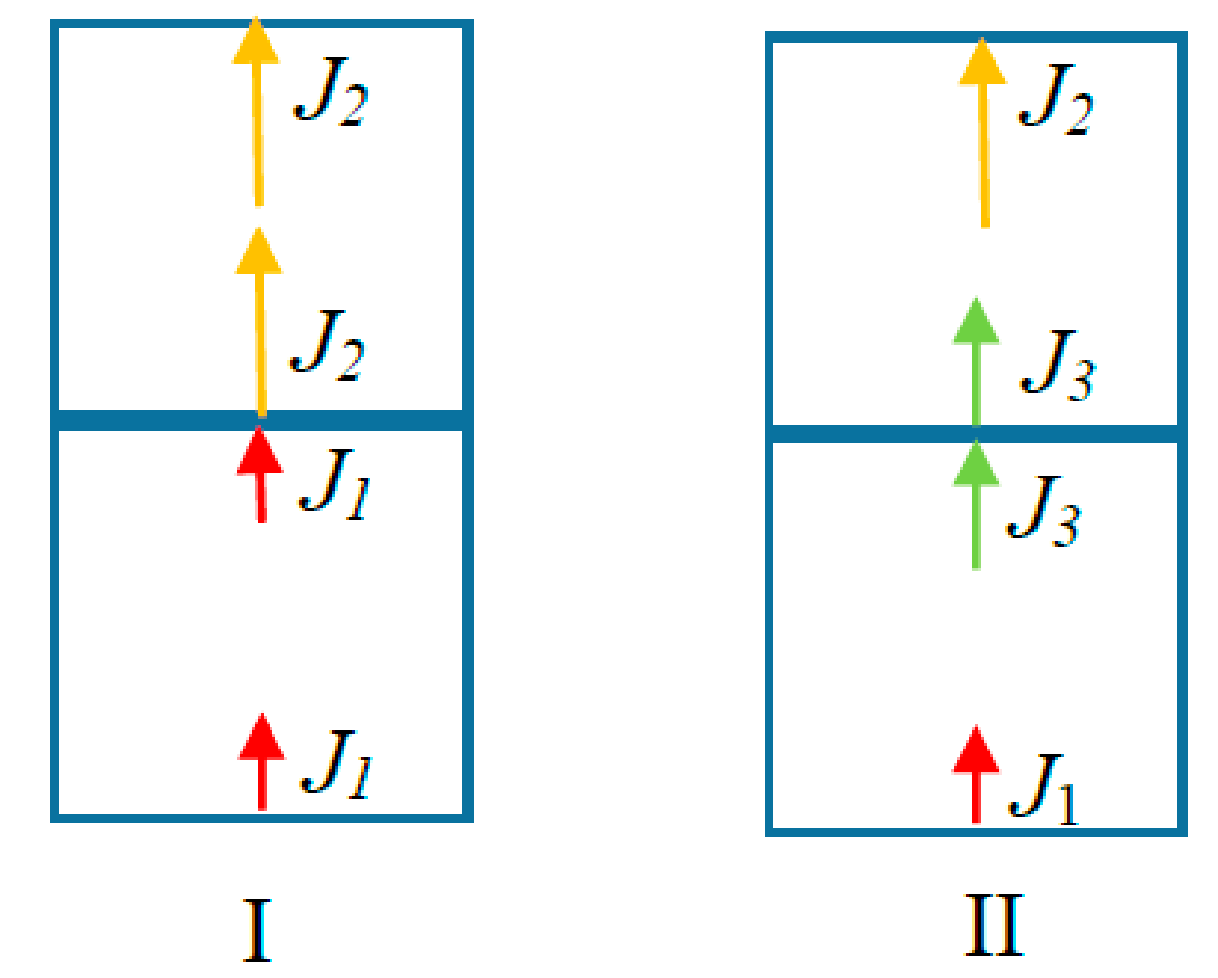
The temporal variation of currents and their movement in the volume $V$ under consideration give rise to an electromagnetic field, and there are two ways to write down the equations pertinent to it. In both procedures, the volume where the current density and the speed of propagation are defined is divided into a matrix of small cubical volumes. In the first procedure, the current and velocity are assumed not to change within a given elementary volume. The changes take place at the boundary where the elementary volumes are connected to each other. That is, if the current is changing in space, then charges will accumulate at the boundary of the elements. In the second procedure, the changes take place inside the elementary volume, but the current and the speed remain continuous across the boundary. Thus, no charges accumulate at the boundary. Of course, if there are conducting bodies inside the volume of space, they have to be taken care of using correct boundary conditions. This concept is outlined in Figure 1, where the events taking place across two elementary volumes are depicted for clarity. Of course, the final equations resulting from the two procedures may appear different, but they both give rise to the same total field.

2.1. Generalization Based on Current Discontinuity at the Boundary—Procedure I

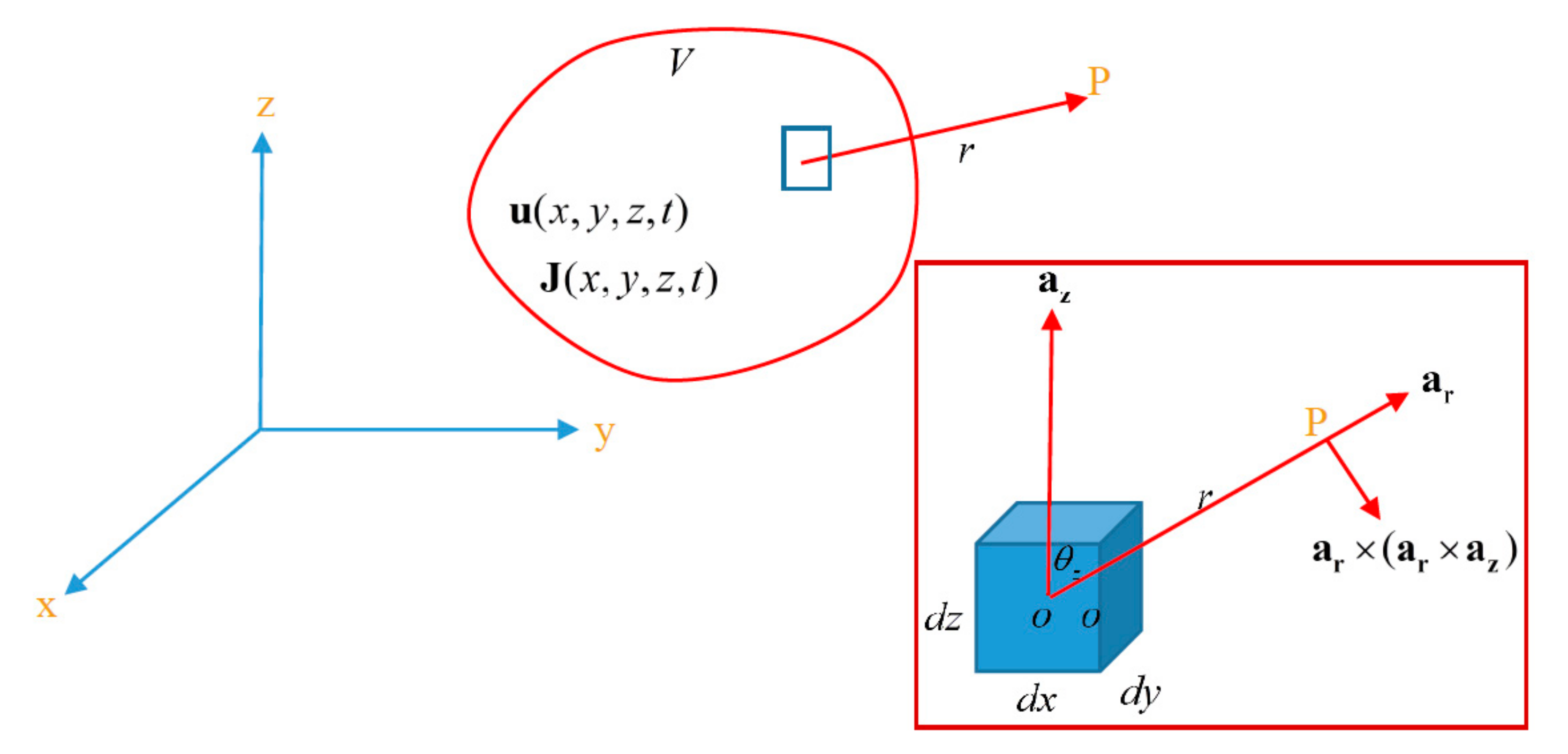
Let us consider a small cubical volume element $dv$ located inside the volume $V$ where the current density and velocity of propagation are defined. The relevant geometry is defined in Figure 2. In the analysis to follow, we will first write down the expressions for the electric field produced by the currents flowing along the z-axis inside the elementary volume. The total electric field produced by the z-directed currents is then obtained by summing up the contributions from all the elementary volumes. Once this is done, the expressions for the electric fields produced by the x and y-directed currents are written down directly using the derived results as an analogy.

Let us consider the electric field produced by the currents propagating along the z-axis inside the volume element. We assume that the current is initiated at the bottom of the cubical element (i.e., at the surface $z-dz/2$), propagates without any change across the element, and terminates at the top of the element (i.e., at the surface $z+dz/2$). The contribution to the electric field due to this current flow across the cubical element has three components: radiation, static, and velocity fields. The radiation field is produced by the acceleration of charges at the ends of the cubical element. The static field and the velocity field are different forms of the Coulomb field produced by charges. The static field is the Coulomb field produced by the stationary charges that will accumulate at the ends of the current element as the current continues to flow. The velocity field is the modified Coulomb field that incorporates the effect of the movement of charges. This field term reduces to the static field when the velocity of the charge goes to zero. Thus, in principle, the total field is given by the sum of the Coulomb fields and the radiation fields. The expressions for the field terms pertinent to the propagation of currents along a given axis were previously obtained by Cooray and Cooray [3,5,8], and those results are utilized here.

The initiation of the z-directed current at one end of the current element (i.e., at the surface $z-dz/2$) and its termination at the other end (i.e., at the surface $z+dz/2$) give rise to acceleration and deceleration of charges resulting in a radiation field. The radiation field at point P generated by the acceleration and deceleration of charges at the ends of the current element is given by Cooray and Cooray [8], and it is given below. Note that, as stated earlier, for brevity in writing down the corresponding equations, we have suppressed the explicit mention of the spatial dependence in the current density by writing $J_x(x,y,z,t)\Rightarrow J_x(t)$).

$$\begin{gathered} d{E}_{r,z}(t)=\frac{dv }{4\pi {\epsilon }_o{c}^{2}r} \\ \left\{\frac{\partial J_z(t-r/c)}{\partial t}-\frac{2u_z\cos {\theta }_z}{r(1-\frac{u_z}{c}\cos {\theta }_z)}z{J}_z(t-r/c)+\frac{u_z^2{\sin }^2{\theta }_z}{rc{(1-\frac{u_z}{c}\cos {\theta }_z)}^2}{J}_z(t-r/c)\right\}\left(a_z\times a_r\right)\times a_r \end{gathered}$$

(1)

In the above equations, $dv=dz.dx.dy$ (i.e., the volume of the current element). Remember that $a_z$ is the unit vector directed along the z-direction. In this case it coincides with the unit vector $a_u$ directed along the direction of propagation of the current. Note that $a_r$ is defined locally, with origin at the current element, and not at the origin of a global coordinate system. As the current flows along the z-axis of the element, charges accumulate at the two ends of the channel element. The static field component generated by the charges accumulated at the ends of the current channel is given by [8]:

$$\begin{gathered} d{E}_{s,z}(t)=\frac{dv}{4\pi {\epsilon }_o{r}_{}^2}\left\{\frac{\cos {\theta }_z}{c}{J}_z(t-r/c)-\frac{1}{u}{J}_z(t-r/c)+\frac{2\cos {\theta }_z}{ r}{\displaystyle \underset{0}{\overset{t}{\int }}{J}_z(\tau -r/c)d\tau }\right\}{a}_r \\ +\frac{dv}{4\pi {\epsilon }_o{r}_{}^2}\left\{\frac{1}{r}{\displaystyle \underset{0}{\overset{t}{\int }}{J}_z(\tau -r/c)d\tau }\right\}\left(a_z\times a_r\right)\times a_r. \end{gathered}$$

(2)

The component of the electric field attributable to the velocity field generated as the current pulse propagates along the current element can be written as [8]:

$$d{E}_{v,z}=\frac{J_z(t-r/c)\left\{1-\frac{u_z^2}{c^2}\right\}}{4\pi {\epsilon }_o{r}^2{\left[1-\frac{u_z}{c}\cos {\theta }_z\right]}^2}\left[\frac{a_r}{u}-\frac{a_z}{c}\right]dv.$$

(3)

In references [5,8] it was shown that the sum of these field components will add up to the field expressions corresponding to a time domain infinitesimal dipole of length $dz$. That is, the sum of these field expressions leads to:

$$\begin{array}{c}d{E}^z=\frac{dv}{4\pi {\epsilon }_0}\left[\frac{1}{c^{2}r}\frac{d{J}_z(t-r/c)}{dt}+\frac{1}{c{r}^2}{J}_z(t-r/c)\right.\left.+\frac{1}{r^3}{\displaystyle \underset{0}{\overset{t}{\int }}{J}_z(\tau -r/c)d\tau }\right]\hspace{0.17em}\left(a_z\times a_r\right)\times a_r\\ +\frac{\cos {\theta }_{z}dv}{4\pi {\epsilon }_{0}c}\left[\frac{2}{r^2}{J}_z(t-r/c)+\frac{2c}{r^3}{\displaystyle \underset{0}{\overset{t}{\int }}{J}_z(\tau -r/c)d\tau }\right]\hspace{0.17em}{a}_r.\end{array}$$

(4)

As pointed out in references [5] and [8], note that the field expressions given above correspond to the field expressions of an infinitesimal dipole directed along the z-direction in the time domain. The field term that varies as $1/r$ is the dipole-radiation field, the field term that varies as $1/r^2$ is the dipole-induction field, and the field term that varies as $1/r^3$ is the dipole-static field. It is also pointed out in the above references that Equations (1), (2), and (3) describe the fields associated with the state of the charge that gives rise to the fields. The field term given by Equation (1) is produced by acceleration of charges, the field term given by Equation (2) is produced by stationary charges, and the field term given by Equation (3) is produced by moving charges. Once they are combined to produce Equation (4), this physical association disappears. Note also that the field expressions given by Equations (1) to (3) depend explicitly on the speed of propagation of the current pulse, whereas Equation (4) does not depend explicitly on the speed of propagation.

As noted above there are two ways to express the electric field produced by the z-component of the current in volume V. The electric field can be separated into the components produced by the various physics processes that give rise to electromagnetic fields (Equations (1), (2), and (3)), or it can be written in terms of the dipole fields (Equation (4)).

2.1.1. Field Expressions Pertinent to the Physical Processes Associated with the Generation of Electromagnetic Fields

The total electric field, separated into the components produced by accelerating charges, stationary charges, and moving charges, produced by the z-component of the current located inside the volume V is given by:

$$\begin{gathered} E_r^z(t)={\displaystyle \underset{V}{\iiint }\frac{dv }{4\pi {\epsilon }_o{c}^{2}r}} \\ \left\{\frac{\partial J_z(t-r/c)}{\partial t}-\frac{2u_z\cos {\theta }_z}{r(1-\frac{u_z}{c}\cos {\theta }_z)}{J}_z(t-r/c)+\frac{u_z^2{\sin }^2{\theta }_z}{rc{(1-\frac{u_z}{c}\cos {\theta }_z)}^2}{J}_z(t-r/c)\right\}\left(a_z\times a_r\right)\times a_r; \end{gathered}$$

(5)

$$\begin{gathered} E_s^z(t)={\displaystyle \underset{V}{\iiint }\frac{dv}{4\pi {\epsilon }_o{r}_{}^2}}\left\{\frac{\cos {\theta }_z}{c}{J}_z(t-r/c)-\frac{1}{u_z}{J}_z(t-r/c)+\frac{2\cos {\theta }_z}{ r}{\displaystyle \underset{0}{\overset{t}{\int }}{J}_z(\tau -r/c)d\tau }\right\}{a}_r \\ +{\displaystyle \underset{V}{\iiint }\frac{dv}{4\pi {\epsilon }_o{r}_{}^2}}\left\{\frac{1}{r}{\displaystyle \underset{0}{\overset{t}{\int }}{J}_z(\tau -r/c)d\tau }\right\}\left(a_z\times a_r\right)\times a_r; \end{gathered}$$

(6)

$$E_v^z={\displaystyle \underset{V}{\iiint }\frac{J_z(t-r/c)\left\{1-\frac{u_z^2}{c^2}\right\}}{4\pi {\epsilon }_o{r}^2{\left[1-\frac{u_z}{c}\cos {\theta }_z\right]}^2}\left[\frac{a_r}{u_z}-\frac{a_z}{c}\right]dv}.$$

(7)

Equations (5), (6), and (7) express the fields produced by accelerating charges, static charges, and moving charges, respectively, associated with the z-component of the current in the volume V. In an analogous manner, the field components generated by the x-component of the current are given by:

$$\begin{gathered} E_r^x(t)={\displaystyle \underset{V}{\iiint }\frac{dv }{4\pi {\epsilon }_o{c}^{2}r}} \\ \left\{\frac{\partial J_x(t-r/c)}{\partial t}-\frac{2u_x\cos {\theta }_x}{r(1-\frac{u_x}{c}\cos {\theta }_x)}{J}_x(t-r/c)+\frac{u_x^2{\sin }^2{\theta }_x}{rc{(1-\frac{u_x}{c}\cos {\theta }_x)}^2}{J}_x(t-r/c)\right\}\left(a_x\times a_r\right)\times a_r; \end{gathered}$$

(8)

$$\begin{gathered} E_s^x(t)={\displaystyle \underset{V}{\iiint }\frac{dv}{4\pi {\epsilon }_o{r}_{}^2}}\left\{\frac{\cos {\theta }_x}{c}{J}_x(t-r/c)-\frac{1}{u_x}{J}_x(t-r/c)+\frac{2\cos {\theta }_x}{ r}{\displaystyle \underset{0}{\overset{t}{\int }}{J}_x(\tau -r/c)d\tau }\right\}{a}_r \\ +{\displaystyle \underset{V}{\iiint }\frac{dv}{4\pi {\epsilon }_o{r}_{}^2}}\left\{\frac{1}{r}{\displaystyle \underset{0}{\overset{t}{\int }}{J}_x(\tau -r/c)d\tau }\right\}\left(a_x\times a_r\right)\times a_r; \end{gathered}$$

(9)

$$E_v^x={\displaystyle \underset{V}{\iiint }\frac{J_x(t-r/c)\left\{1-\frac{u_x^2}{c^2}\right\}}{4\pi {\epsilon }_o{r}^2{\left[1-\frac{u_x}{c}\cos {\theta }_z\right]}^2}\left[\frac{a_r}{u_x}-\frac{a_x}{c}\right]dv}.$$

(10)

Similarly, the field components generated by the y-component of the current are given by:

$$\begin{gathered} E_r^y(t)={\displaystyle \underset{V}{\iiint }\frac{dv }{4\pi {\epsilon }_o{c}^{2}r}} \\ \left\{\frac{\partial J_y(t-r/c)}{\partial t}-\frac{2u_y\cos {\theta }_y}{r(1-\frac{u_y}{c}\cos {\theta }_y)}{J}_y(t-r/c)+\frac{u_y^2{\sin }^2{\theta }_y}{rc{(1-\frac{u_y}{c}\cos {\theta }_y)}^2}{J}_y(t-r/c)\right\}\left(a_y\times a_r\right)\times a_r; \end{gathered}$$

(11)

$$\begin{gathered} E_s^y(t)={\displaystyle \underset{V}{\iiint }\frac{dv}{4\pi {\epsilon }_o{r}_{}^2}}\left\{\frac{\cos {\theta }_y}{c}{J}_y(t-r/c)-\frac{1}{u_y}{J}_y(t-r/c)+\frac{2\cos {\theta }_y}{ r}{\displaystyle \underset{0}{\overset{t}{\int }}{J}_y(\tau -r/c)d\tau }\right\}{a}_r \\ +{\displaystyle \underset{V}{\iiint }\frac{dv}{4\pi {\epsilon }_o{r}_{}^2}}\left\{\frac{1}{r}{\displaystyle \underset{0}{\overset{t}{\int }}{J}_y(\tau -r/c)d\tau }\right\}\left(a_y\times a_r\right)\times a_r; \end{gathered}$$

(12)

$$E_v^y={\displaystyle \underset{V}{\iiint }\frac{J_y(t-r/c)\left\{1-\frac{u_y^2}{c^2}\right\}}{4\pi {\epsilon }_o{r}^2{\left[1-\frac{u_y}{c}\cos {\theta }_y\right]}^2}\left[\frac{a_r}{u_y}-\frac{a_y}{c}\right]dv}.$$

(13)

These field components can be combined into a single vector equation as follows (note that $J=J_x{a}_x+J_y{a}_y+J_z{a}_z$ and $u=u\cdot a_u$).

$$\begin{gathered} E_r^{}(t)={\displaystyle \underset{V}{\iiint }\frac{dv }{4\pi {\epsilon }_o{c}^{2}r}} \\ \left\{\frac{\partial J(t-r/c)}{\partial t}\times a_r-\frac{2u\cdot a_r}{r(1-\frac{u\cdot a_r}{c})}J(t-r/c)\times a_r+\frac{{\left|u\times a_r\right|}^2}{rc{(1-\frac{u\cdot a_r}{c})}^2}J(t-r/c)\times a_r\right\}\times a_r; \end{gathered}$$

(14)

$$\begin{gathered} E_s^{}(t)={\displaystyle \underset{V}{\iiint }\frac{dv}{4\pi {\epsilon }_o{r}_{}^2}} \\ \left\{\frac{a_u\cdot a_r}{c}J(t-r/c)\cdot a_u-\frac{1}{u\cdot a_u}J(t-r/c)\cdot a_u+\frac{2a_u\cdot a_r}{ r}{\displaystyle \underset{0}{\overset{t}{\int }}J(t-r/c)\cdot a_{u}d\tau }\right\}{a}_r+{\displaystyle \underset{V}{\iiint }\frac{dv}{4\pi {\epsilon }_o{r}_{}^2}} \\ \left\{\frac{1}{r}{\displaystyle \underset{0}{\overset{t}{\int }}\left(J(\tau -r/c)\times a_r\right)\times a_{r}d\tau }\right\}; \end{gathered}$$

(15)

$$E_v^{}={\displaystyle \underset{V}{\iiint }\frac{J(t-r/c)\cdot a_u\left\{1-\frac{u\cdot a_u}{c^2}\right\}}{4\pi {\epsilon }_o{r}^2{\left[1-\frac{u\cdot a_r}{c}\right]}^2}\left[\frac{a_r}{u_y}-\frac{a_u}{c}\right]dv},$$

(16)

The total electric field separated into radiation, static, and velocity terms is then given by:

$$E(x,y,z,t)=E_r^{}(x,y,z,t)+E_s^{}(x,y,z,t)+E_v^{}(x,y,z,t).$$

(17)

If a charge density that does not vary with time is located inside the volume (for example, the static charges in a thundercloud that do not take part in a lightning discharge), then a static field equal to the one given below (i.e., Equation (18)) has to be added to the above equations.

$$E_{s0}(x,y,z)={\displaystyle \underset{v}{\int }\frac{\rho dv}{4\pi {\epsilon }_0{r}^2}}{a}_r.$$

(18)

That is, the total field in this case is given by:

$$E(x,y,z,t)=E_r(x,y,z,t)+E_s(x,y,z,t)+E_v(x,y,z,t)+E_{s0}(x,y,z).$$

(19)

2.1.2. Dipole Representation

If the dipole field expressions in Equation (4) are used to represent the electric fields, the total electric field produced by the z-current distribution located inside the volume $V$ is then given by:

$$\begin{array}{c}{E}^z={\displaystyle \underset{V}{\iiint }\frac{dv}{4\pi {\epsilon }_0}\left[\frac{1}{c^{2}r}\frac{d{j}_z(t-r/c)}{dt}+\frac{1}{c{r}^2}{j}_z(t-r/c)\right.\left.+\frac{1}{r^3}{\displaystyle \underset{0}{\overset{t}{\int }}{j}_z(\tau -r/c)d\tau }\right]\hspace{0.17em}(a_z\times a_r)\times a_r}\\ \hspace{1em}+{\displaystyle \underset{V}{\iiint }\frac{\cos {\theta }_{z}dv}{4\pi {\epsilon }_{0}c}\left[\frac{2}{r^2}{j}_z(t-r/c)+\frac{2c}{r^3}{\displaystyle \underset{0}{\overset{t}{\int }}{j}_z(\tau -r/c)d\tau }\right]\hspace{0.17em}{a}_r}.\end{array}$$

(20)

Following the same procedure, the electric fields produced by the x- and y-directed currents in the volume can be written as:

$$\begin{array}{c}{E}^x={\displaystyle \underset{V}{\iiint }\frac{dv}{4\pi {\epsilon }_0}\left[\frac{1}{c^{2}r}\frac{d{j}_x(t-r/c)}{dt}+\frac{1}{c{r}^2}{j}_x(t-r/c)\right.\left.+\frac{1}{r^3}{\displaystyle \underset{0}{\overset{t}{\int }}{j}_x(\tau -r/c)d\tau }\right]\hspace{0.17em}(a_x\times a_r)\times a_r}\\ \hspace{1em}+{\displaystyle \underset{V}{\iiint }\frac{\cos {\theta }_{x}dv}{4\pi {\epsilon }_{0}c}\left[\frac{2}{r^2}{j}_x(t-r/c)+\frac{2c}{r^3}{\displaystyle \underset{0}{\overset{t}{\int }}{j}_x(\tau -r/c)d\tau }\right]\hspace{0.17em}{a}_r};\end{array}$$

(21)

$$\begin{array}{l}{E}^y={\displaystyle \underset{V}{\iiint }\frac{dv}{4\pi {\epsilon }_0}\left[\frac{1}{c^{2}r}\frac{d{j}_y(t-r/c)}{dt}+\frac{1}{c{r}^2}{j}_y(t-r/c)\right.\left.+\frac{1}{r^3}{\displaystyle \underset{0}{\overset{t}{\int }}{j}_y(\tau -r/c)d\tau }\right]\hspace{0.17em}(a_y\times a_r)\times a_r}\\ \end{array}$$

(22)

$\hspace{1em}+{\displaystyle \underset{V}{\iiint }\frac{\cos {\theta }_{y}dv}{4\pi {\epsilon }_{0}c}\left[\frac{2}{r^2}{j}_y(t-r/c)+\frac{2c}{r^3}{\displaystyle \underset{0}{\overset{t}{\int }}{j}_y(\tau -r/c)d\tau }\right]\hspace{0.17em}{a}_r}$.

As before, if a charge density that does not vary with time is located inside the volume, then a static field equal to the one given by Equation (18) has to be added to the above equations. That is, the total field is given by:

$$E(x,y,z,t)=E^x(x,y,z,t)+E^y(x,y,z,t)+E^z(x,y,z,t)+E_{s0}(x,y,z).$$

(23)

One can see immediately that the field components given by Equations (20), (21), and (22) are nothing but the generalized dipole fields.

One can combine Equations (20), (21), and (22) into a single vector equation, resulting in:

$$\begin{gathered} E(x,y,z,t)=\frac{1}{4\pi {\epsilon }_0}{\displaystyle \underset{v}{\int }dv{\displaystyle \underset{0}{\overset{t}{\int }}\frac{2(J(\tau -r/c)\cdot a_r)a_r+(J(\tau -r/c)\times a_r)\times a_r}{r^3}}}d\tau \\ +\frac{1}{4\pi {\epsilon }_0}{\displaystyle \underset{v}{\int }\left\{\frac{2(J(t-r/c)\cdot a_r)a_r+(J(t-r/c)\times a_r)\times a_r}{c{r}^2}\right\}}dv \\ +\frac{1}{4\pi {\epsilon }_0}{\displaystyle \underset{v}{\int }\left\{\frac{\partial J(t-r/c)/\partial t\times a_r)\times a_r}{c^{2}r}\right\}dv}+\frac{1}{4\pi {\epsilon }_0}{\displaystyle \underset{v}{\int }\frac{\rho a_r}{r^2}dv}. \end{gathered}$$

(24)

It is of interest to note that the above expressions are identical to those derived by Shao [9]. In reference [8], using a lightning return stroke as an example, it was shown that the sum of the expressions given by Equations (14), (15), and (16) gives the same total field as the expression given by Equation (24).

2.2. Generalization Based on Current Continuity at the Boundary—Procedure II

We will consider the same volume of space where the current densities and the velocity of propagation are given as a function of space and time. As described earlier, we will divide the volume where the current densities and velocities are specified into elementary cubical volumes. Consider a cubical volume element located at any arbitrary point (x,y,z). As in the previous case, we will derive the field equations pertinent to the current flow along the z-direction, and the corresponding equations pertinent to current flow along the x- and y-directions will be given directly using the z-direction analogy. Recall that in this procedure we assume that currents and speeds change inside the volume element but remain continuous across boundaries between elements. As the current propagates across the volume element, a certain fraction of the current is reduced or gained. The amount of current lost or gained by the elementary cubicle volume as the current propagates along the element along the z-direction is given by:

$$\frac{d{I}_z(t)}{dz}=dxdy\left[\frac{\partial J_z(t)}{\partial z}+\frac{1}{u_z}\frac{\partial J_z(t)}{\partial t}\right].$$

(25)

Observe that this is the same expression used to estimate the current that is being lost into the corona sheath (i.e., corona current) in the Modified Transmission Line with Exponential Decay (MTLE) and the Modified Transmission Line with Linear Decay (MTLL) return stroke models [10,11]. The total current lost within the elementary volume is then given by:

$$d{I}_z(t)=dv\left[\frac{\partial J_z(t)}{\partial z}+\frac{1}{u_z}\frac{\partial J_z(t)}{\partial t}\right].$$

(26)

As the current propagates along the volume element, a fraction of the velocity of propagation is also changed, and the amount of velocity reduction is given by:

$$d{u}_z=dz\frac{\partial u_z}{\partial z}.$$

(27)

We are now in a position to write down the electric fields produced by the volume element. First note that the loss (or gain) of charge and the reduction (or increase) in the velocity of propagation within the volume will give rise to radiation fields. The radiation field produced by the change in current in the volume element is given by [3,5,8]:

$$d{E}_{r,i}^z=\frac{\Delta I_z(t-r/c)u_z}{4\pi {\epsilon }_o{c}^{2}r}\frac{1}{\left[1-\frac{u_z\cos {\theta }_z}{c}\right]}(a_z\times a_r)\times a_r.$$

(28)

The radiation field produced by the change in velocity is given by:

$$d{E}_{r,v}^z=\frac{\Delta u_z{J}_z(t-r/c)dxdy}{4\pi {\epsilon }_o{c}^{2}r}\frac{1}{\left[1-\frac{u_z\cos {\theta }_z}{c}\right]}(a_z\times a_r)\times a_r.$$

(29)

Combining these two equations we will find the total radiation produced by the volume element as:

$$\begin{array}{l}d{E}_r^z=\frac{dv}{4\pi {\epsilon }_o{c}^{2}r\left[1-\frac{u_z\cos {\theta }_z}{c}\right]}\\ \left[u_z\frac{\partial J_z(t-r/c)}{\partial z}+\frac{\partial J_z(t-r/c)}{\partial t}+J_z(t-r/c)\frac{\partial u_u}{\partial z}\right](a_z\times a_r)\times a_r\end{array}$$

(30)

Due to the loss (or gain) of current, a certain amount of charge is gained (or lost) by the volume element. This charge as a function of time is given by:

$$d{Q}_z(t)=dv{\displaystyle \underset{0}{\overset{t}{\int }}\left[\frac{\partial J_z}{\partial z}+\frac{1}{u_z}\frac{\partial J_z}{\partial t}\right]}d\tau .$$

(31)

The static field produced by this charge at the point of observation is:

$$d{E}_s^z=\frac{dv{\displaystyle \underset{0}{\overset{t}{\int }}\left[\frac{\partial J_z(t-r/c)}{\partial z}+\frac{1}{u_z}\frac{\partial J_z(t-r/c)}{\partial t}\right]}d\tau }{4\pi {\epsilon }_o{r}_{}^2}\hspace{0.17em}{a}_r.$$

(32)

The velocity field produced by the propagation of current across the element is identical to the one obtained for the elementary volume in procedure I. That is, the velocity field produced by the volume element is:

$$d{E}_v^z=\frac{J_z(t-r/c)\left\{1-\frac{u_z^2}{c^2}\right\}}{4\pi {\epsilon }_o{r}^2{\left[1-\frac{u_z}{c}\cos {\theta }_z\right]}^2}\left[\frac{a_r}{u_z}-\frac{a_z}{c}\right]dv.$$

(33)

Thus, the total electric field produced by the volume element is

$$\begin{gathered} d{E}_{}^z=\frac{dv}{4\pi {\epsilon }_o{c}^{2}r\left[1-\frac{u_z\cos {\theta }_z}{c}\right]}\left[u_z\frac{\partial J_z(t-r/c)}{\partial z}+\frac{\partial J_z(t-r/c)}{\partial t}+J_z(t-r/c)\frac{\partial u_u}{\partial z}\right](a_z\times a_r)\times a_r \\ +\frac{dv{\displaystyle \underset{0}{\overset{t}{\int }}\left[\frac{\partial J_z(t-r/c)}{\partial z}+\frac{1}{u_z}\frac{\partial J_z(t-r/c)}{\partial t}\right]}d\tau }{4\pi {\epsilon }_o{r}_{}^2}\hspace{0.17em}{a}_r \\ +\frac{dv\hspace{0.17em}{J}_z(t-r/c)\left\{1-\frac{u_z^2}{c^2}\right\}}{4\pi {\epsilon }_o{r}^2{\left[1-\frac{u_z}{c}\cos {\theta }_z\right]}^2}\left[\frac{a_r}{u_z}-\frac{a_z}{c}\right]. \end{gathered}$$

(34)

The total electric field produced by the total volume V is then given by:

$$\begin{gathered} E_{}^z={\displaystyle \underset{V}{\iiint }}\frac{dv}{4\pi {\epsilon }_o{c}^{2}r\left[1-\frac{u_z\cos {\theta }_z}{c}\right]}\frac{\left[u_z\frac{\partial J_z(t-r/c)}{\partial z}+\frac{\partial J_z(t-r/c)}{\partial t}+J_z(t-r/c)\frac{\partial u_u}{\partial z}\right]}{4\pi {\epsilon }_o{c}^{2}r}(a_z\times a_r)\times a_r \\ +{\displaystyle \underset{V}{\iiint }}\frac{dv{\displaystyle \underset{0}{\overset{t}{\int }}\left[\frac{\partial J_z(t-r/c)}{\partial z}+\frac{1}{u_z}\frac{\partial J_z(t-r/c)}{\partial t}\right]}d\tau }{4\pi {\epsilon }_o{r}_{}^2}\hspace{0.17em}{a}_r \\ +{\displaystyle \underset{V}{\iiint }}\frac{dv\hspace{0.17em}{J}_z(t-r/c)\left\{1-\frac{u_z^2}{c^2}\right\}}{4\pi {\epsilon }_o{r}^2{\left[1-\frac{u_z}{c}\cos {\theta }_z\right]}^2}\left[\frac{a_r}{u_z}-\frac{a_z}{c}\right]. \end{gathered}$$

(35)

Using the same analogy, the electric fields produced by the currents propagating along the x-and y-directions are given by:

$$\begin{gathered} E_{}^x={\displaystyle \underset{V}{\iiint }}\frac{dv}{4\pi {\epsilon }_o{c}^{2}r\left[1-\frac{u_x\cos {\theta }_x}{c}\right]}\frac{\left[u_x\frac{\partial J_x(t-r/c)}{\partial z}+\frac{\partial J_x(t-r/c)}{\partial t}+J_x(t-r/c)\frac{\partial u_x}{\partial z}\right]}{4\pi {\epsilon }_o{c}^{2}r}(a_x\times a_r)\times a_r \\ +{\displaystyle \underset{V}{\iiint }}\frac{dv{\displaystyle \underset{0}{\overset{t}{\int }}\left[\frac{\partial J_x(t-r/c)}{\partial z}+\frac{1}{u_x}\frac{\partial J_x(t-r/c)}{\partial t}\right]}d\tau }{4\pi {\epsilon }_o{r}_{}^2}\hspace{0.17em}{a}_r \\ +{\displaystyle \underset{V}{\iiint }}\frac{dv\hspace{0.17em}{J}_x(t-r/c)\left\{1-\frac{u_x^2}{c^2}\right\}}{4\pi {\epsilon }_o{r}^2{\left[1-\frac{u_x}{c}\cos {\theta }_x\right]}^2}\left[\frac{a_r}{u_x}-\frac{a_x}{c}\right]; \end{gathered}$$

(36)

$$\begin{gathered} E_{}^y={\displaystyle \underset{V}{\iiint }}\frac{dv}{4\pi {\epsilon }_o{c}^{2}r\left[1-\frac{u_y\cos {\theta }_y}{c}\right]}\frac{\left[u_y\frac{\partial J_y(t-r/c)}{\partial z}+\frac{\partial J_y(t-r/c)}{\partial t}+J_y(t-r/c)\frac{\partial u_y}{\partial z}\right]}{4\pi {\epsilon }_o{c}^{2}r}(a_y\times a_r)\times a_r \\ +{\displaystyle \underset{V}{\iiint }}\frac{dv{\displaystyle \underset{0}{\overset{t}{\int }}\left[\frac{\partial J_y(t-r/c)}{\partial z}+\frac{1}{u_y}\frac{\partial J_y(t-r/c)}{\partial t}\right]}d\tau }{4\pi {\epsilon }_o{r}_{}^2}\hspace{0.17em}{a}_r \\ +{\displaystyle \underset{V}{\iiint }}\frac{dv\hspace{0.17em}{J}_y(t-r/c)\left\{1-\frac{u_y^2}{c^2}\right\}}{4\pi {\epsilon }_o{r}^2{\left[1-\frac{u_y}{c}\cos {\theta }_y\right]}^2}\left[\frac{a_r}{u_z}-\frac{a_y}{c}\right]. \end{gathered}$$

(37)

These three equations can be combined into one single vector equation, resulting in the following.

$$\begin{gathered} E={\displaystyle \underset{V}{\iiint }}\frac{dv}{4\pi {\epsilon }_o{c}^{2}r\left[1-\frac{u\cdot a_r}{c}\right]}\frac{\left[\frac{\partial J(t-r/c)\cdot u}{\partial z}+\frac{\partial J(t-r/c)\cdot a_u}{\partial t}\right]}{4\pi {\epsilon }_o{c}^{2}r}(a_u\times a_r)\times a_r \\ +{\displaystyle \underset{V}{\iiint }}\frac{dv{\displaystyle \underset{0}{\overset{t}{\int }}\left[\frac{\partial J(t-r/c)}{\partial z}+\frac{1}{u\cdot a_u}\frac{\partial J(t-r/c)}{\partial t}\right]}\cdot a_{u}d\tau }{4\pi {\epsilon }_o{r}_{}^2}\hspace{0.17em}{a}_r \\ +{\displaystyle \underset{V}{\iiint }}\frac{dv\hspace{0.17em}J(t-r/c)\left\{1-\frac{{(u\cdot a_u)}^2}{c^2}\right\}\cdot a_u}{4\pi {\epsilon }_o{r}^2{\left[1-\frac{u\cdot a_r}{c}\right]}^2}\left[\frac{a_r}{u_z}-\frac{a_u}{c}\right]. \end{gathered}$$

(38)

The first term gives the electric field produced by accelerating charges, the second term gives the electric field produced by stationary charges, and the third term gives the electric field produced by moving charges. If the volume contains a charge density that does not vary with time, then, as indicated previously, the static field produced by this charge, as given by Equation (18), has to be added to the above field equations.

3. Application of the Two Techniques to Calculate the Electromagnetic Fields from a Lightning Channel

The electric field calculation procedures presented in this paper can be used to evaluate electric fields produced by volume current distributions. The technique to adopt (i.e., Procedure I or Procedure II) depends on the way the problem is specified. For example, in problems related to electrical discharges, either in the laboratory or in the Earth’s atmosphere, where the speed of propagation of current pulses is specified, Procedure II can be adopted easily in field calculations. In cases where the speed is not specified and cannot be derived from the given current distribution easily, it is easier to use Procedure I. In the analysis to follow, we will consider the charge and current distributions associated with the transmission line model of lightning return strokes [12]. We have selected this example for two reasons. First, the electromagnetic fields produced by the transmission line model calculated using different techniques are available in the literature, and the results to be obtained can be compared and contrasted with them. Second, in this example, it is easier to visualize the differences in the two procedures of calculation presented in this paper.

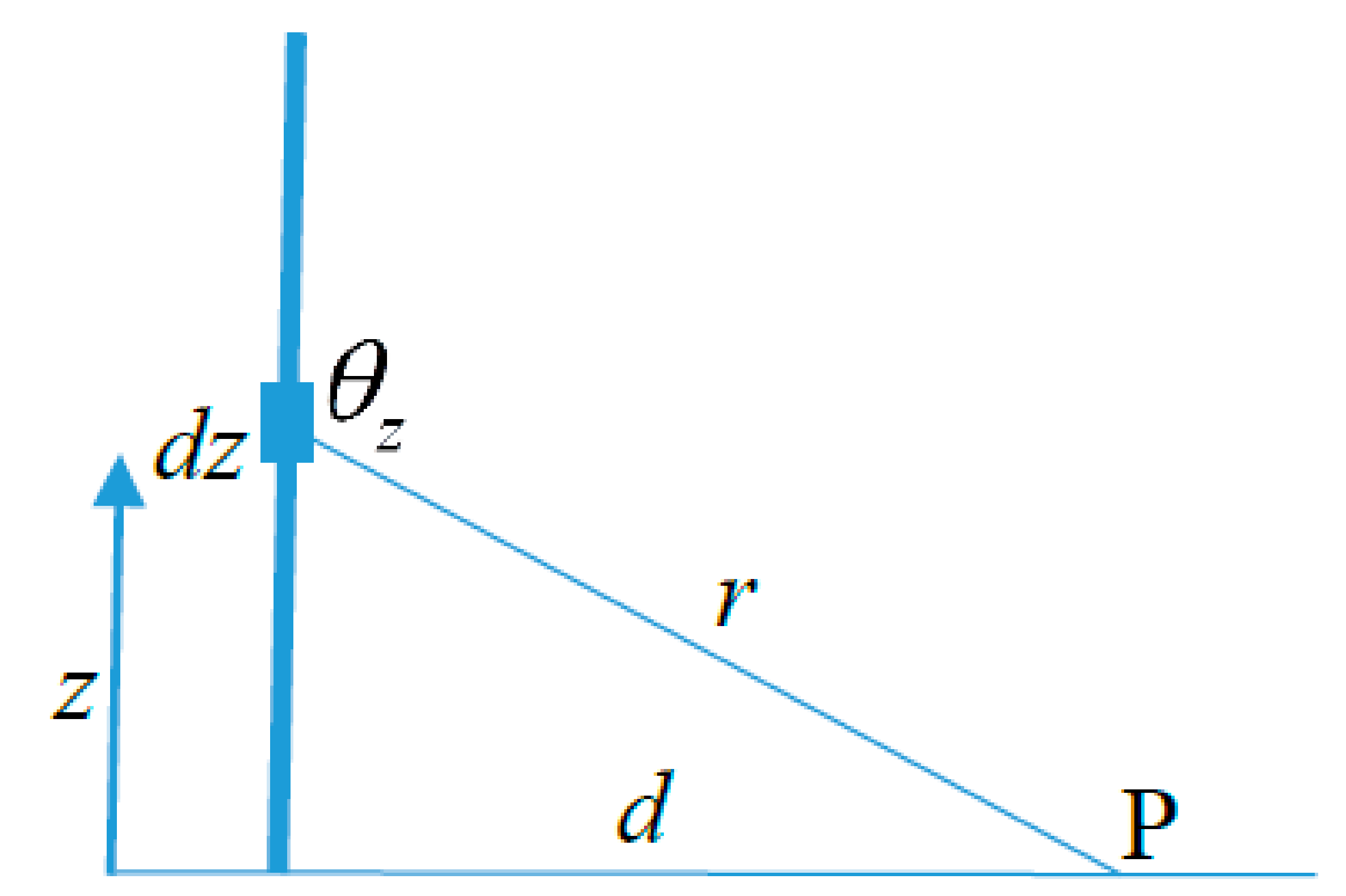
In the transmission line model, a return stroke is represented by a current pulse that propagates from the ground to the cloud with uniform speed and without attenuation. In order to simplify the analysis, it is assumed here that the return stroke speed is equal to the speed of light [13]. Moreover, the lightning channel is assumed to be straight and vertical. We also assume that once the current is initiated at the ground end, it will propagate upwards for a longer time than the duration of the fields of interest. Otherwise, the equations to be presented later have to be modified to take into account the termination of the current at the cloud end of the channel. In the present paper, the electric fields are estimated at ground level at a horizontal distance $d$ from the lightning channel. The relevant geometry is shown in Figure 3. In the analysis, the ground plane is assumed to be perfectly conducting.

In the model, the current density $J_z$(in the problem under consideration, this is only a function of $t$ and $z$) and the velocity of propagation $u_z$ of the current (which is a constant and directed along the z-axis) are given. First, let us divide the return stroke channel into a large number of elementary channel sections of length $dz$. The radius of the channel is denoted by $a$, and the current density is assumed to be distributed uniformly across the cross section of the channel. Using Procedure I, the electric field generated by the channel can be obtained by summing up the contributions to the electric field from all the channel elements. Note that while adopting Procedure I, it is assumed that inside each element the current is generated at the bottom of the element and is terminated at the top of the element. Thus, each element contributes in creating the electric field. The electric field generated by each channel element is given by Equations (20) or (24). Application of these field equations to the problem under investigation leads to the following expressions for the dipole-static, dipole-induction, and dipole-radiation field components at ground level at a distance d from the point of strike (note that the effect of the perfectly conducting ground is taken into account by replacing it with an image channel):

$$E_s(t)=\frac{a}{2\pi {\epsilon }_0}{\displaystyle \underset{0}{\overset{H}{\int }}\frac{2-3{\sin }^2{\theta }_z}{r^3}}{\displaystyle \underset{0}{\overset{t}{\int }}{J}_z(\tau -r/c)d\tau dz};$$

(39)

$$E_i(t)=\frac{a}{2\pi {\epsilon }_0}{\displaystyle \underset{0}{\overset{H}{\int }}\frac{2-3{\sin }^2{\theta }_z}{c{r}^2}}{J}_z(\tau -r/c)dz;$$

(40)

$$E_r(t)=\frac{a}{2\pi {\epsilon }_0}{\displaystyle \underset{0}{\overset{H}{\int }}\frac{{\sin }^2{\theta }_z}{c^{2}r}}\frac{\partial J_z(\tau -r/c)}{\partial t}dz.$$

(41)

The total electric field at the point of observation is given by:

$$E_{z,total}(t)=E_r(t)+E_i(t)+E_s(t).$$

(42)

In the above equations, $J_z(t)$ is the current density at height z.

Let us now apply the equations obtained using the second procedure. Since the speed of propagation of the current is equal to the speed of light, the velocity term generated by each channel element, as given by Equations (35) or (38), is equal to zero. Now, let us consider the radiation term as given by Equation (30). That is, the radiation field generated by a given element is given by:

$$\begin{array}{l}d{E}_r^z=\frac{dv}{4\pi {\epsilon }_o{c}^{2}r{u}_z\left[1-\frac{u_z\cos {\theta }_z}{c}\right]}\\ \left[u_z\frac{\partial J_z(t-r/c)}{\partial z}+\frac{\partial J_z(t-r/c)}{\partial t}+u_z{J}_z(t-r/c)\frac{\partial u_z}{\partial z}\right](a_z\times a_r)\times a_r\end{array}$$

(43)

Let us rewrite the above equation as:

$$\begin{array}{l}d{E}_r^z=\frac{dz}{4\pi {\epsilon }_o{c}^{2}r\left[1-\frac{u_z\cos {\theta }_z}{c}\right]}\\ \left[\frac{\partial I_z(t-r/c)}{\partial z}+\frac{1}{u_z}\frac{\partial I_z(t-r/c)}{\partial t}+I_z(t-r/c)\frac{\partial u_z}{\partial z}\right](a_z\times a_r)\times a_r\end{array}$$

(44)

The total radiation field is then given by:

$$\begin{array}{l}{E}_r^z={\displaystyle \underset{0}{\overset{H}{\int }}}\frac{dz}{4\pi {\epsilon }_o{c}^{2}r\left[1-\frac{u_z\cos {\theta }_z}{c}\right]}\\ \left[\frac{\partial I_z(t-r/c)}{\partial z}+\frac{1}{u_z}\frac{\partial I_z(t-r/c)}{\partial t}+I_z(t-r/c)\frac{\partial u_z}{\partial z}\right](a_z\times a_r)\times a_r\end{array}$$

(45)

In the above equation, $H$ is the height of the return stroke channel. Now, in the case of the transmission line model,

$$\frac{\partial I_z(t-r/c)}{\partial z}+\frac{1}{u_z}\frac{\partial I_z(t-r/c)}{\partial t}=0.$$

(46)

Moreover, the acceleration of the charges takes place only at $z=0$ (i.e., the speed changes from 0 to $u$). Thus, the total radiation field from the return stroke at the point of observation is given by:

$$E_r^z=\frac{u_z{I}_z(t-r/c)}{4\pi {\epsilon }_o{c}^{2}r\left[1-\frac{u_z\cos {\theta }_z}{c}\right]}(a_z\times a_r)\times a_r.$$

(47)

Resolving the field at ground level into vertical and horizontal components, and taking into account the effect of the image current, the radiation field along the z-direction at ground level reduces to:

$$E_{r,P}^z=-\frac{u_z}{2\pi {\epsilon }_o{c}^{2}r}{I}_z(t-r/c)a_z.$$

(48)

Since the speed of propagation is equal to the speed of light, we obtain:

$$E_{r,P}^z=-\frac{1}{2\pi {\epsilon }_{o}cr}{I}_z(t-r/c)a_z.$$

(49)

Note that, since the speed of propagation is equal to the speed of light, the velocity term goes to zero. As a positive current propagates along the channel, the net charge deposited at the point of initiation of the current (the bottom of the channel) cancels due to the image, and, for this reason, the static field produced by this charge goes to zero. At times longer than the time necessary for the propagation of the current all the way to the upper end of the channel, one does have to consider the static field produced by the positive charge that will accumulate at the top of the channel and its image. However, for times shorter than this propagation time, the charge accumulated at the upper end of the channel and its image is zero, and the corresponding static field associated with these charges is also equal to zero. Thus, for times less than the time necessary for propagation of the current along the channel, the net vertical electric field at ground level is given by:

$$E_{Total,P}^z=-\frac{1}{2\pi {\epsilon }_{o}cr}{I}_z(t-r/c)a_z.$$

(50)

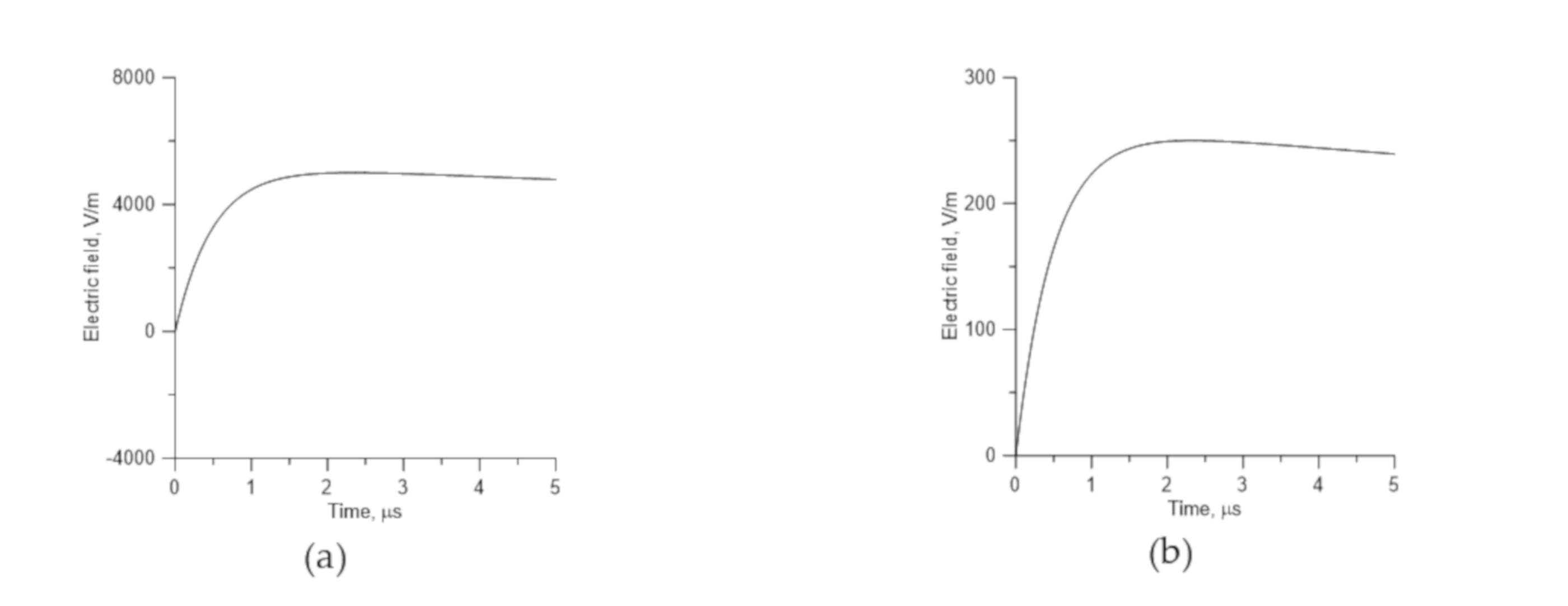
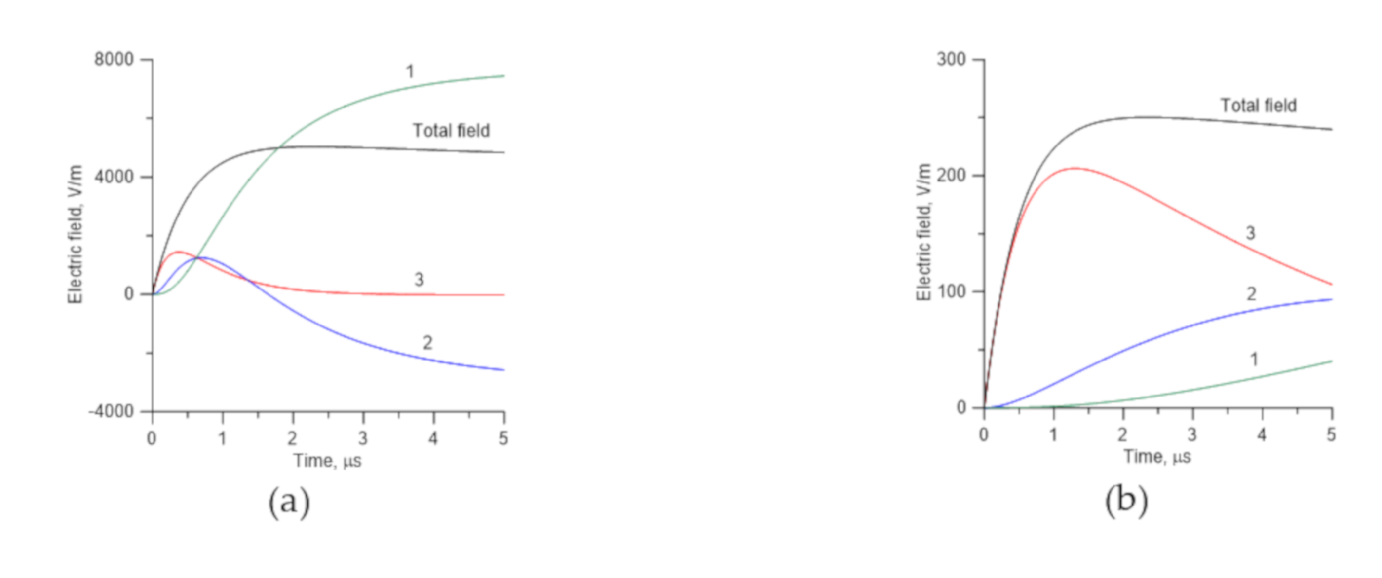
Even though the mathematical expression for the electric field given in Equation (50) is different from the field components given by Equations (39), (40), and (41), all these expressions give rise to the same total electric field. For example, the electric field at distances of 100 m and 2 km, as predicted by Equation (50), is shown in Figure 4. The total electric field and the individual components predicted by Equations (39), (40), and (41) are shown in Figure 5. Note that the sum of field terms given by Equations (39), (40), and (41) predict the same total electric field.

In the analysis presented here, it was assumed that the speed of propagation of the current pulse was equal to the speed of light. This made the analysis much simpler because the velocity field term is zero under these conditions. Of course, one can analyze the problem using a current speed that is lower than the speed of light. In that case, too, the two techniques predict the same total electric and magnetic fields, even though the signatures of the field components that add up to the total field are different.

4. Conclusions

In this paper, we derived generalized equations to calculate the electromagnetic fields of a time varying current distribution using charge acceleration equations. The final field expressions can be written either in terms of the current density and the velocity of propagation of the currents or purely in terms of the current density. In the latter case, the speed of propagation does not enter into the final field expressions, and they become identical to the ones produced by a distribution of short dipoles. Using the transmission line model of the return stroke as an example, it was demonstrated that both expressions gave rise to the same total electric field.