Article

Joint Anomalies of High-Frequency Geoacoustic Emission and Atmospheric Electric Field by the Ground–Atmosphere Boundary in a Seismically Active Region (Kamchatka)

1
Institute of Cosmophysical Research and Radio Wave Propagation Far Eastern Branch of the Russian Academy of Sciences, Paratunka 684034, Russia
2
Institute of Volcanology and Seismology Far Eastern Branch of the Russian Academy of Sciences, Petropavlovsk-Kamchatsky 683006, Russia
*
Authors to whom correspondence should be addressed.
Atmosphere 2019, 10(5), 267; https://doi.org/10.3390/atmos10050267
Submission received: 4 March 2019 / Revised: 26 April 2019 / Accepted: 6 May 2019 / Published: 13 May 2019
(This article belongs to the Special Issue Lithosphere–Atmosphere–Ionosphere Coupling (LAIC) Models)

Abstract

:
The authors generalize and analyze the investigation results of joint anomalies of high-frequency geoacoustic emission and atmospheric electric field by the ground–atmosphere boundary which were detected by them in Kamchatka. These anomalies are observed as geoacoustic emission increases in kilohertz frequency range and bay-like decreases of atmospheric electric field with the sign change which occur close in time during calm weather conditions. It is the authors’ opinion that the common nature of these anomalies is short-time stretching of the near-surface sedimentary rocks at an observation site during unstable tectono-seismic process. A scheme of the detected anomalies formation has been suggested.

1. Introduction

The boundary between the ground and the atmosphere is characterized by considerable changes of contacting medium properties, large fluxes of mass and energy, a broad list of simultaneously existing heterogeneous fields, and their interactions. At this boundary, the near-surface rocks and the near-ground atmosphere interchange various substances, pulse, and energy. Field interaction manifests in direct and indirect forms when several direct interactions connected between each other are realized. Geodynamic phenomena and processes occurring by the ground–atmosphere boundary are the subject for investigation of an intensively developing new subdiscipline “Near-surface geophysics” [1,2].
The characteristic features of the ground–atmosphere boundary and the adjacent earth crust and atmospheric layer are anomalous disturbances of different fields in seismically active regions. They are usually recorded within the interval up to one month before an earthquake with the magnitude of more than 4–5 at the distance up to the low hundreds of kilometers from an epicenter and are interpreted as precursors [3,4]. It is generally accepted that these disturbances are associated with rock deformations during earthquake preparation.
Among the preseismic anomalies of the near-surface fields, increase of high-frequency geoacoustic emission in kilohertz frequency range [5,6,7,8,9] and bay-like decrease of atmospheric electric field with sign change during calm weather conditions [10,11,12,13,14,15] are observed. Anomalies of these fields, essentially different, occur in solid and air mediums and have different polarity that indicates various mechanisms of formation. Just like precursors in other fields, they are initiated by geomechanical stress field change in a zone of earthquake preparation and are generated in the result of transformation, near-surface rocks stress—deformation.
In this case, geoacoustic emission anomalies are rock direct responses and atmospheric electric field anomalies are the indirect responses of the near-ground air electric state on deformation caused by an earthquake preparation process. Common deformation nature of these anomalies is the reason that they occur close in time.
Seismic process is a sequence of rock constant deformation under the influence of tectonic forces. Thus, anomalies of geoacoustic emission and atmospheric electric field are observed in a seismically active region not only before an earthquake but during near-surface rocks deformation intensification within seismically calm periods. It is also confirmed by the mutual interaction and significant correlation between near-surface fields variations in an aseismic region [1], where the tectonic energy inflow and rock deformation rate are significantly less. Instability of the tectono-seismic process in time and mottled hierarchic block structure of the earth crust determine the complicated spatial-time deformation of rocks, including local tension and compression which should cause different responses of high-frequency geoacoustic emission and atmospheric electric field.
Joint investigation of geoacoustic emission and atmospheric electric field has not been carried out up to the present time. It is important for understanding of the earth crust impact on the near-ground atmosphere in seismically active regions, for detection of an earthquake complex precursor and for investigation of the formation mechanisms of the near-surface fields disturbances during the tectono-seismic process.
In the paper we generalize and analyze the investigation results of the detected joint anomalies of high-frequency geoacoustic emission and atmospheric electric field by the ground–atmosphere boundary on Kamchatka peninsula. Simultaneous geoacoustic and atmospheric electric measurements were carried out at two sites during different time intervals in summer–autumn 2005–2009 and 2012. They were carried out together with the measurements of the main meteorological quantities applying the same observation method and one measuring-recording complex. In 2009 the measurements were accompanied by the observations of the earth surface deformation. In 2012 the radon and thoron volumetric activity was measured in the near-surface ground layer gas. That allowed us to obtain qualitatively new set of experimental data, discussion and analysis of which are useful for the investigation of near-surface fields interaction during the tectono-seismic process.

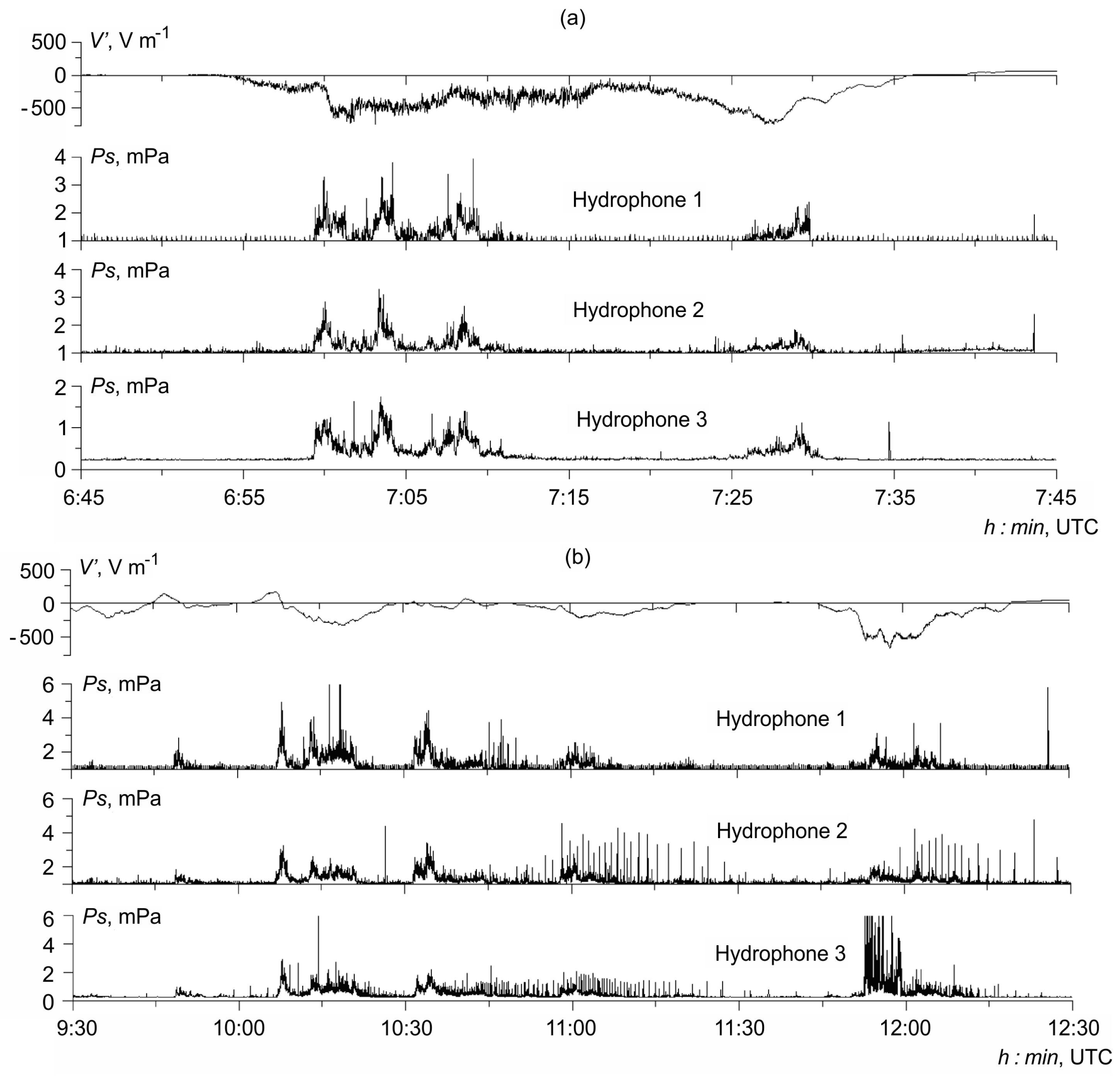
2. Observations and Results

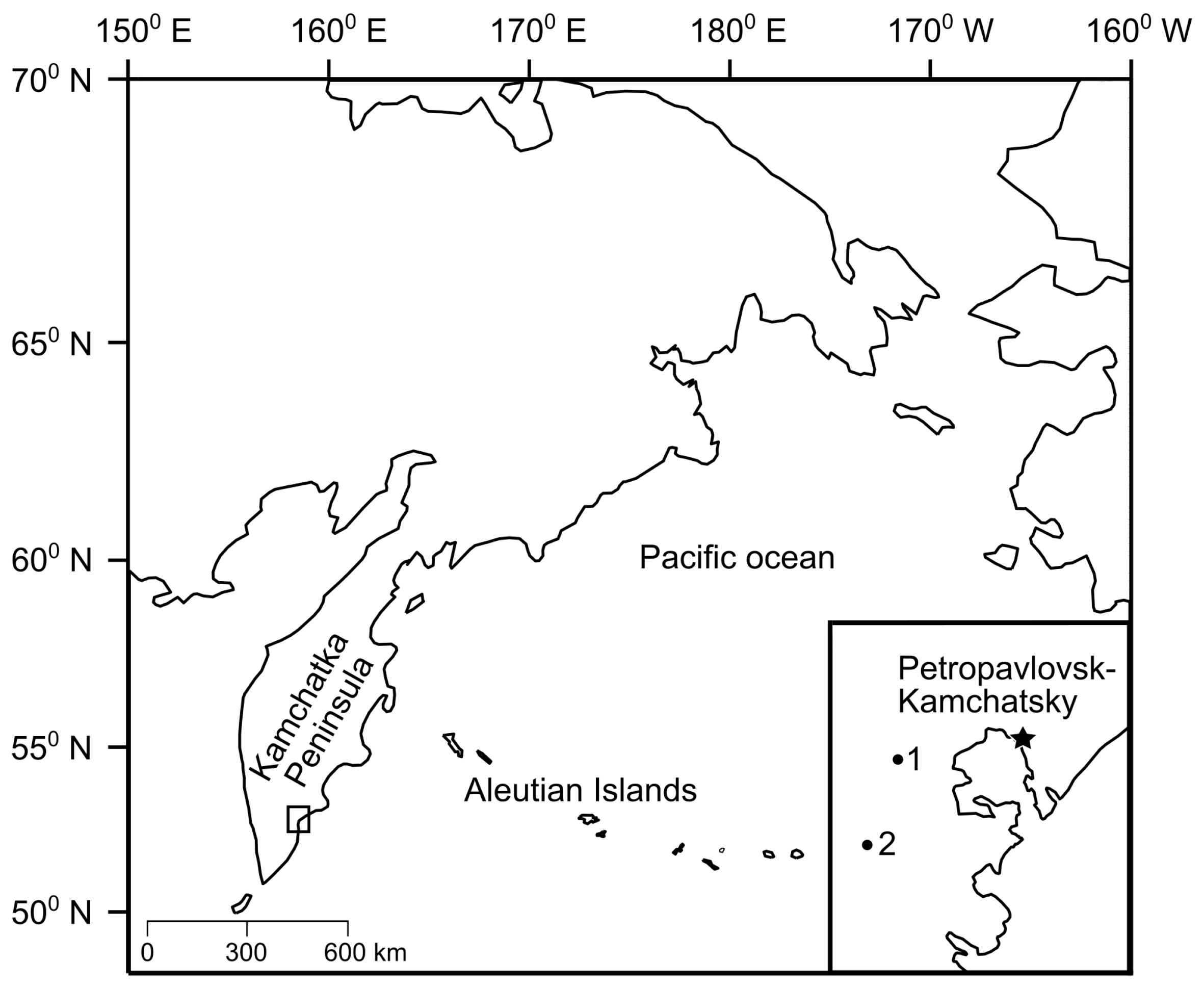
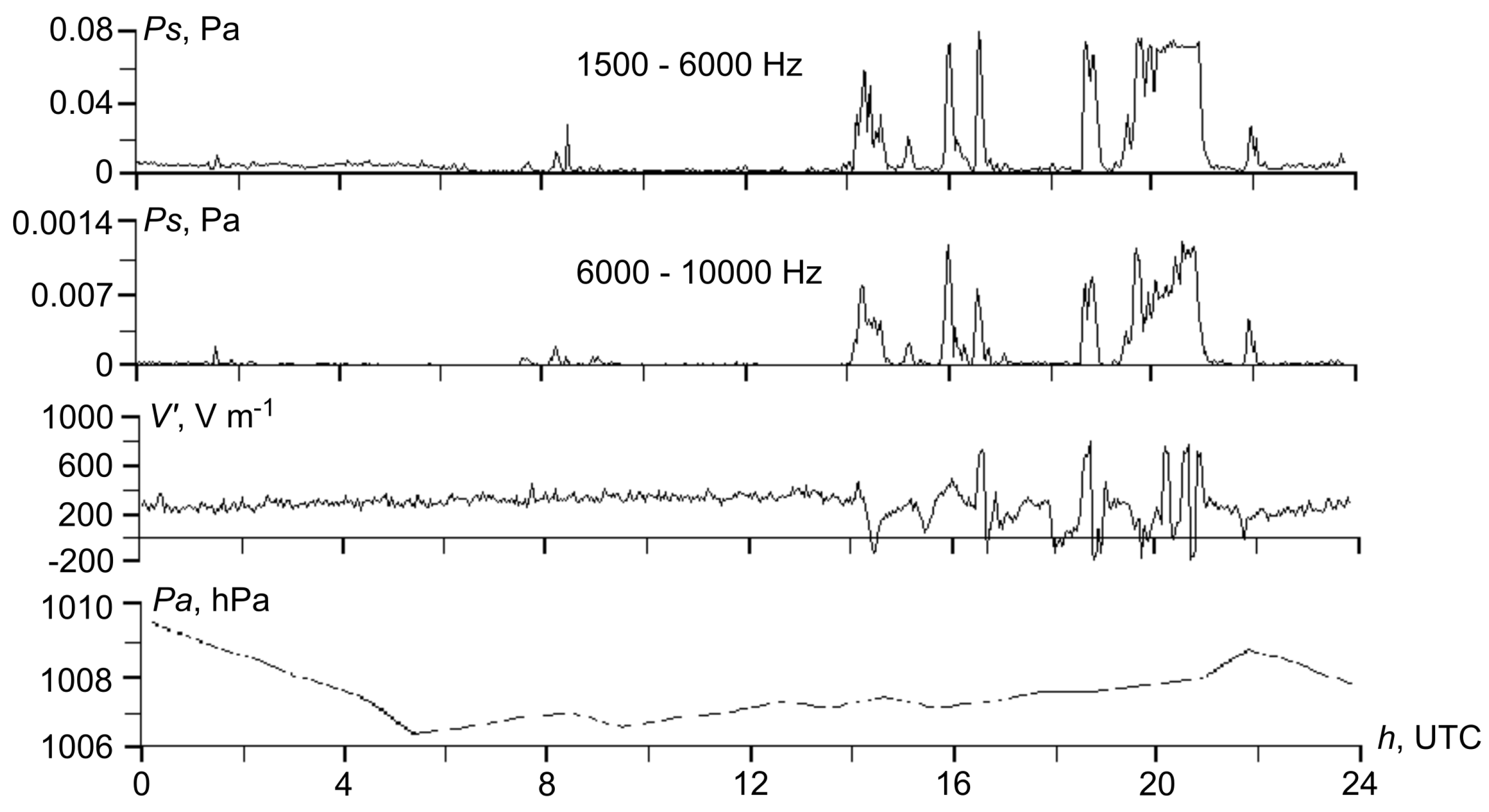
2.1. Observations at “Mikizha” Site

For the first time simultaneous measurements of geoacoustic emission and atmospheric electric field were carried out at “Mikizha” site (52.99 ° N, 158.23 ° E, Figure 1) from 23 August to 11 October 2005 (experiment 2005). They were realized in the conditions without industrial noise and airborne pollution which significantly affect the atmospheric electric field behavior by the ground. A piezoceramic hydrophone, installed at the height of 10 cm above the Mikizha lake bottom, was used as a geoacoustic emission sensor. The lake dimensions are 200 × 700 m 2 . Its inmost depth where the hydrophone is installed is 4 m. Geoacoustic signals were recorded at the frequency ranges of 0.1–10, 10–50, 50–200, 200–700, 700–1500, 1500–6000, 6000–10,000 Hz. Acoustic pressure P s accumulated over 4-s period in each range was considered [16].
Atmospheric electric field potential gradient V was measured by a rotational electrostatic fluxmeter which had sensitivity of about 3 V·m 1 and the setting time at the level of 0.9 was 1 s. The fluxmeter primary transducer was installed 130 m away from the hydrophone on the shore of Mikizha lake on an open meadow which is a part of a large flat field with low plant stand. It was partially placed in an open cavity of the size of 0.3 × 0.3 m 2 and the depth of 0.4 m. The measuring plate of the electrostatic generator was at the height of 7 cm above the ground. V was measured once in 4-s period. Air pressure, wind velocity, and rain intensity were measured 20 m away from the fluxmeter. The sensors were at the heights of 2.5, 4.9 and 4.2 m from the ground, respectively.
Applying a data acquisition digital system developed by the authors based on a PC, all the measured quantities were recorded continuously. To eliminate the mutual influence of geoacoustic and atmospheric electric data, signals from the hydrophone and the electrostatic fluxmeter arrived at different analogue-digital converters (16- and 14-bit, respectively).
During the measurements, disturbances, which are close in time, of acoustic pressure P s and of atmospheric electric field potential gradient V were recorded. They were observed in calm weather conditions (weakly changing air pressure, absence of rain and wind of more than 6 m·s 1 ) when there was no significant impact of meteorological factors on P s and V behavior. Such disturbances were recorded during seismically calm periods and before a local earthquake that indicates their tectono-seismic nature. During seismically calm periods, potential gradient V disturbances were observed during significant disturbances of acoustic pressure, with sudden commencement, occurring only in kilohertz frequency range, as a rule (Figure 2). Joint disturbances of P s and V before an earthquake are illustrated in Figure 3. This earthquake with the magnitude of 4.8 mb occurred on 9 September 2005 at 11:42 UTC at the epicentral distance of 260 km from “Mikizha” site. The hypocenter coordinates are 51.060 ° N, 156.153 ° E; the depth is 136 km (NEIC, http://earthquake.usgs.gov). To illustrate the high-frequency character of acoustic disturbance, P s behavior is represented at the frequencies of 50–200 and 6000–10,000 Hz. It is clear from Figure 3 that a sudden P s increase begins at the frequencies of 6000–10,000 Hz 21 h before the earthquake. However, there is no such an increase at the frequencies of 50–200 Hz. Potential gradient V disturbance begins almost simultaneously. Anomalous disturbances of these quantities cease 7.5 h before the earthquake. The weather turned nasty several hours after it [16].
Investigation of geoacoustic emission and atmospheric electric field was continued in summer–autumn 2006–2008. The measured quantities, the observation method, the acquisition, and record system were the same. The measurements were carried out from 27 June to 16 October 2006 (experiment 2006), from 28 June to 24 October 2007 (experiment 2007) and from 2 July to 27 October 2008 (experiment 2008) [17]. In the result of long geoacoustic measurements [7] and our measurements during the experiment 2005, it was established that anomalous geoacoustic disturbances manifest the most brightly at the frequency range of 2.0–6.5 kHz at “Mikizha” site. Thus, acoustic pressure P s accumulated over 4-s period in this range was considered.
The characteristic feature of joint anomalies of high-frequency geoacoustic emission and atmospheric electric field is the field decrease often with a sign change followed by a recovery almost to the same level. Such a bay-like decreases of potential gradient V manifest the most during significant increases of acoustic pressure P s which, as a rule, have sudden commencement and last for more than several minutes. It occurs in calm weather conditions, i.e., slightly changing air pressure without rain and strong or moderate wind [17]. Figure 4 illustrate the record fragment of joint anomalies of potential gradient V and acoustic pressure P s . There was no rain during the period represented in Figure 4. During a strong P s increase at about 15:00 UTC on 22 August 2006 (Figure 4) the potential gradient V decreased to −120 V·m 1 .
Anomalous disturbances of acoustic pressure P s and of potential gradient V have different form and usually last from the first tens of minutes to the first hours. As a rule, they cover a part of one hour, of two adjacent hours or that of the first and the last hours when lasting for several hours. Disturbances of such duration manifest in the changeability P s ¯ of V ¯ and hourly mean values which, in our case, are the averages from 900 values. Application of hourly mean values simplifies data large volume analysis and allows us to state the presence or the absence of the relation between high-frequency geoacoustic emission disturbances and those of atmospheric electric field.
To clarify the weather effect on the behavior of geoacoustic emission and atmospheric electric field, we considered the correlations between P s ¯ , V ¯ series and hourly mean values of meteorological quantities (air pressure P a ¯ , its temperature T ¯ and relative humidity F ¯ , wind velocity U ¯ , and rain intensity I ¯ ) which are the averages from 6 values. To choose an appropriate method for analysis, all the series were verified on normalcy of distribution. It turned out that P s ¯ , V ¯ , U ¯ , I ¯ , series are distributed abnormally and P a ¯ , T ¯ and F ¯ series have almost normal distribution. Thus, Spearman nonparametric correlation analysis was applied [17].
Figure 5 illustrates cross-correlation functions for the series of P s ¯ and V ¯ hourly mean values. The shifted series is V ¯ . It is clear from Figure 5 that the functions values are negative in all the experiments and their maximum values are observed during V ¯ zero shifts. Consequently, V ¯ negative disturbances occurred simultaneously with P s ¯ disturbances with the accuracy up to one hour. Thus, P s ¯ and V ¯ paired hourly mean values were considered. Scatterplots between these values are shown in Figure 6a–c.
The relations of non-meteorological origin between the disturbances of geoacoustic emission and atmospheric electric field were detected by the method suggested by the authors. To remove bad weather effects, we considered only those pairs of hourly mean values of acoustic pressure P s ¯ and potential gradient V ¯ when there was no rain ( I ¯ = 0 ), strong or moderate wind ( U ¯ < 1.5 m·s 1 ), low air pressure ( P a ¯ > 995 hPa) during the corresponding hours. Scatterplots between P s ¯ and V ¯ during such calm weather conditions are illustrated in Figure 6d–f.
In the author’s opinion [18], the relation between P s ¯ and V ¯ , represented in Figure 6d–f contains two components, they are: a background component determined by weak effect of uncounted meteorological and other factors on geoacoustic emission and atmospheric electric field and a tectonic nature component. The latter is generated by geoacoustic emission and electric field anomalies different in sign which occur during intensification of near-surface rocks deformation in the region of measurement point. Such intensification should occur multiply during unstable in time and intensive tectono-seismic process taking place by the Eastern Kamchatka.
We consider that the background component of the relation manifests when P s ¯ is less than some value P s * ¯ and the tectonic component manifests when P s ¯ is more than P s * ¯ that indicates near-surface rocks deformation intensification. Different mechanisms of formation of the relation background and tectonic components, particularly determined by different mediums in which geoacoustic and atmospheric electric anomalies (near-surface rocks and near-ground air) occur, cause a complicated dependence between P s ¯ and V ¯ . To separate the background and the tectonic components, piecewise linear regression and quasi-Newtonian method were applied to estimate its parameters. Acoustic pressure discontinuity point, which corresponds to P s * ¯ value at first approximation, was calculated by STATISTICA software package.
In the experiments 2006, 2007 and 2008, P s * ¯ was 2.66, 0.46 and 0.41 mPa, respectively. Less values of P s * ¯ in the experiments 2007 and 2008 are explained by acoustic noise level decrease after the experiment 2006 when the hydrophone was taken up for routine maintenance and reinstalled by the bottom several meters away from the previous place. In the result, the noise average level decreased. It was largely determined by inhomogeneous structure of near-bottom sedimentary rocks.
For the datasets illustrated in Figure 6d–f, the Spearman’s correlation coefficient between V ¯ and P s ¯ in the experiments 2006, 2007, and 2008 is 0.08 , 0.32 and 0.04 , respectively. For the same datasets, in case of piecewise linear regression V ¯ on P s ¯ , the multiple correlation coefficient is larger and is 0.77, 0.77 and 0.75, respectively. Consequently, the piecewise linear regression characterizes better the relation between V ¯ and P s ¯ , thus, separation of the indicated datasets into two parts and analysis of the correlation for each of them are reasonable. The parameters of the background and tectonic components of the relation between V ¯ and P s ¯ are shown in Table 1.
It is clear from Table 1 that there is a statistically highly significant component of the relation in the experiments 2006 and 2007 which is absent in the experiment 2008.
The relation between the hourly mean values of potential gradient V ¯ and acoustic pressure P s ¯ in the tectonic component were also analyzed by Kendall’s rank correlation coefficient τ , which allows one to estimate the probability of multidirectional G = ( 1 τ ) / 2 and unidirectional Q = ( 1 + τ ) / 2 changes of two variables. Estimates of the parameter values are illustrated in Table 2.
Based on it, in the experiments 2006, 2007 the correlation coefficient τ is nonzero and its significance level is p < 0.001 . Here G > Q , in other words the possibility of multidirectional changes of V ¯ and P s ¯ , which correspond to opposite in sign anomalous disturbances of atmospheric electric field and geoacoustic emission, is higher. There is no such a tectonic component of the relation between V ¯ and P s ¯ , generated by these disturbances, in experiment 2008.

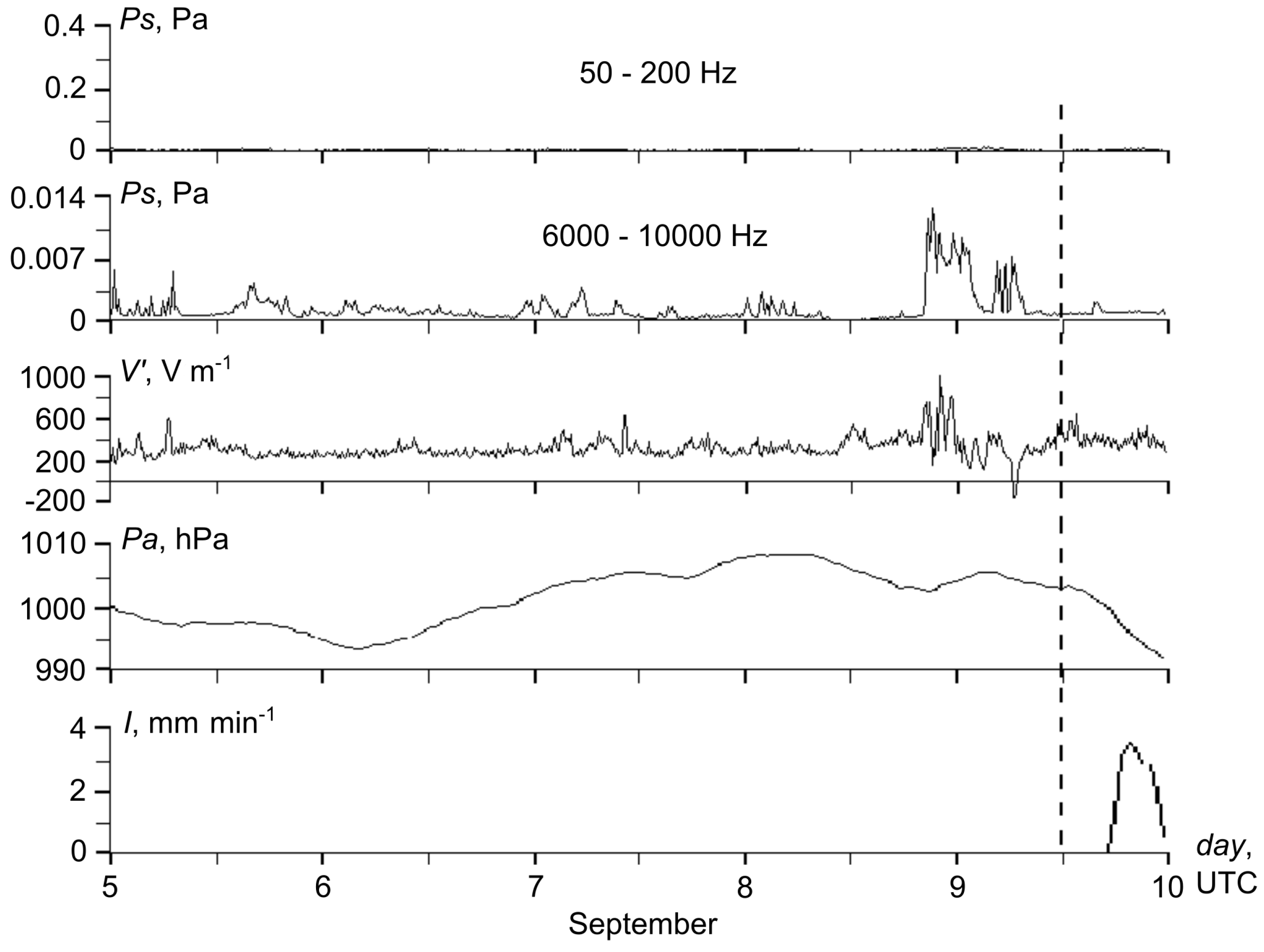
2.2. Observations at “Karymshina” Site
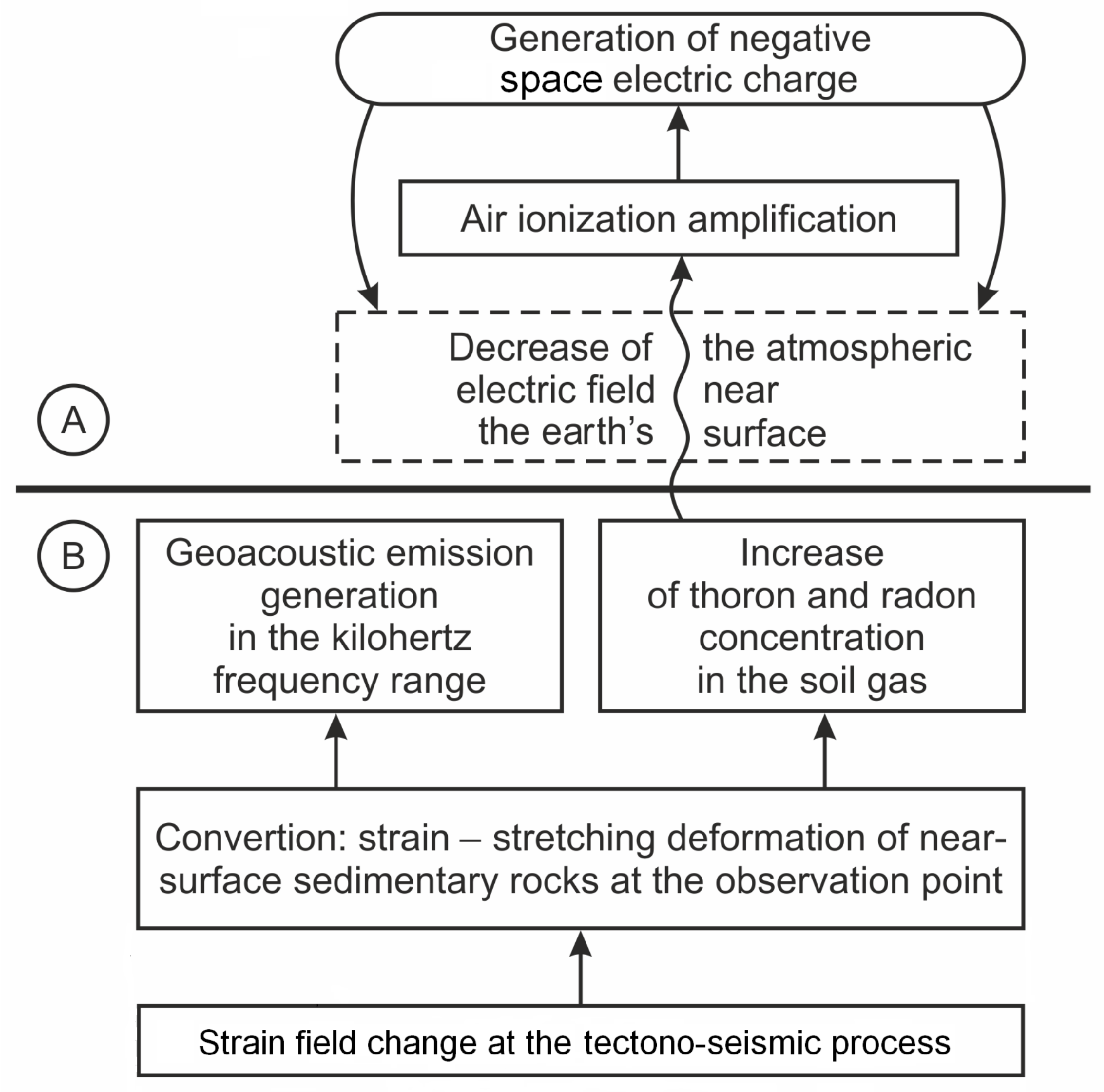
In the authors’ opinion [18], the most probable cause of the relation between the electric field and geoacoustic emission in the tectonic component is the near-surface rocks deformation intensification in the region of measurement point. To verify this fact, simultaneous measurements of ground surface deformation are required. They were carried out on 1–18 October 2009 (experiment 2009) at “Karymshina” site (52.83 ° N, 158.13 ° E, Figure 1), which is located 20 km from “Mikizha” site [19].
Geoacoustic emission was measured by a piezoceramic hydrophone similar to that used in the experiments 2005–2008. The hydrophone was installed in an artificial reservoir 1 × 1 × 1 m 3 in size and covered from rain and wind influence. It was discovered before [7,20] that at “Karymshina” site the geoacoustic emission anomalies manifest the most in the frequency range of 0.7–2.0 kHz. Thus, acoustic pressure P s accumulated in this range over 4-s period was considered.
Atmospheric electric field potential gradient V was measured by the rotational electrostatic fluxmeter which was used in the experiments 2005–2008. The primary transducer of the fluxmeter was installed just in the same way as for those experiments. It was placed 60 m from the hydrophone in the center of a flat glade 20 × 20 m 2 in size surrounded by bushes of about 3 m high. In such conditions, wind weakens near the ground surface and its influence on electric field behavior decreases.
To register the relative deformation of the ground surface ε , a laser strainmeter-interferometer was used. Its measuring base length is 18 m and the sensitivity is 10 11 m. The measurement frequency was 860 Hz, and the accuracy was not less than 10 7 taking into account the weather factors [20,21]. To analyze the ε behavior, first differences were applied. They were calculated by two adjacent values averaged on second interval. They were considered to be the estimates of rock deformation rate ε ˙ . The meteorological quantities were measured once in 10–minute interval at the height of 7 m from the surface.
During slightly changing air pressure, without rain and strong wind, five cases of joint disturbances of acoustic pressure P s and atmospheric potential gradient V were recorded. These disturbances occurred during multiple sign-variable shifts of near-surface rocks which occurred at the background of their comparatively slow tension (Figure 7a,b). Such sifts were recorded at “Karymshina” site before [20] and are clearly seen in the figure of rocks deformation rate ε ˙ graph. We should note the relation between the disturbances P s , V and ε ˙ which is the most noticeable at 18:00–19:00 UTC on 16 October (Figure 7b). It indicates the fact that occurrences of P s and V disturbances depend on near-surface rocks tension rate. Potential gradient V disturbances were recorded as a decrease with sign change followed by the recovery almost to the same level (Figure 7a) and additional increase after the recovery (Figure 7b). In the four recorded cases of rocks compression, only acoustic pressure disturbances occurred despite the same deformation rates and weather conditions [19].
Occurrences of joint anomalies of geoacoustic emission and atmospheric electric field are associated with some substance which is present during near-surface rocks tension, acoustic signal generation, and electric field decrease near the ground surface. In our understanding, this substance is radon and thoron radioactive emanations which are continuously generated in rocks and diffuse into the atmosphere everywhere [22]. When incoming into the atmosphere, they increase the ground air ionization and conductivity that is accompanied by atmospheric electric field decrease by the surface in fair weather conditions [23]. Radon and thoron content in soil gas depends, in particular, on rocks deformation and increases there and in the near-ground air before earthquakes [3,24,25,26,27].
Taking this into consideration, measurements of geoacoustic emission, atmospheric electric field, air pressure, wind velocity and rain intensity were accompanied by the measurements of radon and thoron volumetric activity from 27 August to 17 October 2012 (experiment 2012) [28]. Acoustic pressure P s was recorded in the frequency range of 0.7–2.0 kHz with 4-s data accumulation. Tree piezoceramic hydrophones similar to that used in the experiments 2005–2009 were in operation. They were arranged in the form of a triangle at the distance of 10–35 m from each other and installed in artificial water reservoirs just like in the experiment 2009.
Atmospheric electric field potential gradient V was measured by an electrostatic fluxmeter used in the experiments 2005–2009. Gas for the measurements of radon and thoron volumetric activity was extracted from an open cavity where a primary transducer was partially placed. The cavity promotes emanation accumulation that makes the measurements easier. Gas sample volume was 8% from the unconfined space in the cavity, thus we can neglect the extraction effect on radon and thoron inflow.
Radon and thoron volumetric activity was measured once in 30 min by an automated radiometer with the sensitivity of not less than 1.4 × 10 4 s 1 · Bq 1 · m 3 , 30% limit of the allowable relative error and the average level of its own background of 5 and 0.1 Bq·m 3 for radon and thoron, respectively. The radiometer and the fluxmeter were installed at the distance of 50 m from the hydrophones. Meteorological quantities were measured once in 1 minute at the distance of 8 m from the ground 140 m from the radiometer and the mill.
During the measurement period of 52 days, significant increase of radon R n and thoron T n volumetric activity was observed on 2 October. It considerably exceeded the background level. Acoustic pressure P s increase and atmospheric potential gradient V decrease with sign change were recorded almost at the same time. Variations of R n , T n , P s , V , wind velocity and air pressure on 2 October are illustrated in Figure 8. It is clear from Figure 8 that P s increase at all the measurement points and V decrease with sign change occurred about three hours after R n and then T n increased. They occurred in calm weather conditions without rain, strong or moderate wind, during weakly changing air pressure that indicates non-meteorological nature of these disturbances. Such joint increases of R n , T n , P s and decrease of V with sign change were not simultaneously observed during the measurements any more.
Figure 9 shows a detailed view of the partial time lags of potential gradient V and acoustic pressure P s from Figure 8. It is clear from Figure 9 that P s increases at the measurement points occurred almost simultaneously but differed in amplitude and form that is likely to be determined by various responses of sedimentary rocks at these points on the deformation.
Joint anomalous disturbances of radon, thoron, geoacoustic emission and atmospheric electric field on 2 October were observed 13 days before the earthquake with the magnitude of 5.6 mww. It occurred on 15 October at 01:19 UTC at the epicentral distance R = 140 km from “Karymshina” site [29]. The epicenter coordinates are 51.900 ° N, 159.379 ° E, the source depth is 21 km (NEIC, http://earthquake.usgs.gov). The radon and thoron increases which lasted for about 8 h (Figure 8) agree well with the results of the work [26], where increases of these emanations in soil gas were simultaneously observed in an active fault region before earthquakes with the magnitude M L 4.5 , R < 150 km. They usually appeared 1–20 days before an event and had the least duration of 5–7 h. Impulsive radon spikes in soil–gas before weaker earthquakes ( 1.7 M 4.5 ) were described in the work [30].

3. Discussion

During the experiment 2005, joint anomalies of high-frequency geoacoustic emission and atmospheric electric field were firstly recorded. They were observed in the seismically active region during seismically calm periods and before the local earthquake. Statistically highly significant inverse relation between the hourly average values of acoustic pressure and electric field potential gradient was determined during the experiments 2006, 2007. It has non-meteorological origin. These results indicate that such joint disturbances and their relationship with tectono-seismic process are real.
The near-surface rocks at “Mikizha” and “Karymshina” sites are sedimentary. The thickness of this layer is about 50 and 40 m [7]. There is a well No. 99-8 of 19 m depth at “Karymshina” site which is located 120 m from the electrostatic fluxmeter. Its lithologic log is represented by boulder-cobble deposits with sandy-clay filler (0–5 m), block-rubble deposits with clay filler (5–14 m) and boulder-cobble deposits with sandy filler (14–19 m). The statistic water level is 13.7 m. Based on the estimate in the work [17], geoacoustic emission sources are located not more than 37 m from a hydrophone. Thus, anomalous geoacoustic signals are generated in sedimentary rocks over which surface the atmospheric electric field is measured. We should note that sedimentary rocks are widely spread all over the Earth, about 80% of the continents surface are covered by sedimentary rocks [31].
It was discovered in the experiment 2009 that joint anomalies of high-frequency geoacoustic emission and atmospheric electric field occur as responses, which are close in time, on near-surface sedimentary rocks stretching intensification. Sedimentary rocks have complicated polydisperse fluid-saturated porous structure of low strength. During their stretching, new fragment contact surfaces are formed and emanation increases, moreover, isolated pores are opened, and existing cracks extend. In the result, radon and thoron content in the gas of ground layer grows as well as their inflow into the atmosphere. Mechanical stress between rock fragments simultaneously grows that causes local deformation change and, consequently, micro-movements during which acoustic signals are generated.
Increase of radon and thoron inflow from the soil intensifies near-ground air ionization. In fair weather conditions, it is accompanied by the formation of negative electric charge in the air layer from tens of meter fractions to several meters [32,33,34]. Its average density may be about 700 [35], and the highest reaches 1200 [36] and even 3200 pC·m 3 [37] that is comparable with the average density of a space charge in thunder clouds (300–3000 pC·m 3 ) [38]. Near such a significantly negative charge, normal atmospheric electric field decreases and even the sign changes [36,37]. We should note that these results were obtained in an aseismic region where the rocks deformation rate and emanation inflow into the atmosphere are less than that in seismically active regions. The mechanism of formation of an uncompensated negative charge in the result of near-ground air ionization by radon and submicron metal aerosols before an earthquake is considered in the paper [39]. It was shown that during weak turbulent diffusion when radioactive gas is accumulated in a thin layer by the ground surface, air increased ionization is observed in that layer. Under the effect of normal atmospheric electric field, positive ions move downwards from the region of increased ionization and negative ions move upwards. Thus, uncompensated negative charge appears at some height and local electric field of reverse direction is formed. This field is overlapped on normal atmospheric electric field and decreases locally up to the sign change. Such ion separation in space is confirmed by the measurements [40] in which it was discovered that positive volumetric charge reached +800 pC·m 3 at the level of ground surface whereas negative volumetric charge reached 160 pC·m 3 and more at the height of 1 m.
Owing to what has been said before we can state that the causes of the bay-like decreases of atmospheric electric field during tectono-seismic process are generation, dynamics and dissipation of a negative electric charge of emanation origin in the near-ground air. From this position, the relation between the anomalies of geoacoustic emission and electric field is clear. It is realized in the result of presence of radon and thoron which inflow also responds to the tectono-seismic process. It was confirmed by the joint disturbances of radon, thoron, geoacoustic emission, and atmospheric electric field before the local earthquake during the experiment 2012.
After 20-year continuous observations in China [41], negative anomalies of atmospheric electric field were recorded by the ground surface before many earthquakes. They occurred mainly at nighttime when the field was relatively calm, were observed as decreases up to 500 V·m 1 and more and lasted for several hours and more. We should note that small (about 10–20%) decrease of atmospheric electric field without sign change is observed for weak earthquakes [42]. It can be explained by weaker inflow of radon and thoron into the near-ground air and, consequently, weak negative space charge. Based on the work [43], anomalous increase of atmospheric radon before the earthquake in Japan on 17 January 1995 with the magnitude M W = 6 . 9 is associated with rocks deformations of the order 10 8 10 6 . In the experiment 2009 joint anomalies of geoacoustic emission and atmospheric electric field were observed without notable local earthquakes during near-surface sedimentary rocks stretching deformations of the order 10 6 that is two orders higher than those of tidal deformations. Such significant deformations are likely to be associated with the fact that “Karymshina” site is in the zone of different-rank tectonic fault intersection.
Thus, all the results obtained by the authors can be explained by short-time stretching of near-surface sedimentary rocks at the observation site during a tectono-seismic process, which takes place in the lithosphere and causes stress state changes of the earth crust rocks including the near-surface ones. Based on these results, we can suggest a scheme for the formation of joint anomalies of high-frequency geoacoustic emission and atmospheric electric field in the seismically active region (Figure 10). Based on this scheme, anomalies of geoacoustic emission, radon, thoron, and atmospheric electric field have a common deformation nature and common factor, which gives rise to them, is the sedimentary rock fragmentarity and, consequently, high deformability. Radon and thoron response on rocks stretching deformation and inflow into the near-ground air form an indirect relation between the anomalies of geoacoustic emission and atmospheric electric field.

4. Conclusions

Joint anomalies of high-frequency geoacoustic emission and atmospheric electric field by the ground–atmosphere boundary have been detected for the first time in the seismically active region. They are observed in calm weather conditions and are associated with short-time stretching of near-surface sedimentary rocks at the observation site during unstable tectono-seismic process. On the basis of generalization and analysis of the results of theoretical investigations and nature observations described in the literature and taking into account the results of the experiments carried out by the authors in Kamchatka, a scheme of anomalies formation has been suggested.

Author Contributions

Topicality and methodology for the realization of joint geoacoustic and atmospheric electric investigations, Y.M. and O.R.; contributed to the methods, results, analysis and discussion for the acoustic emission and deformation investigations—Y.M., for atmospheric electric and emanations investigations—O.R.; statistical analysis of the obtained data, O.R.; conceptualization of the relation scheme, Y.M. and O.R.; Y.M. and O.R. wrote the manuscript text and contributed to the graphics.

Funding

This research received no external funding.

Acknowledgments

We wish to thank the environmental scientists from Institute of Cosmophysical Research and Radio Wave Propagation Far Eastern Branch of the Russian Academy of Sciences: Mikhail Mishchenko, Igor Larionov, Alexandra Solodchuk for organization and realization of complex observations, for preparation of the data for further analysis, for their help in text editing and manuscript formatting. Yury Kuzmin, scientist from Kamchatka branch of Geophysical Service of the Russian Academy of Sciences, for realization of radon and thoron measurements.

Conflicts of Interest

The authors declare no conflict of interest.

References

  1. Adushkin, V.V.; Spivak, A.A. Near-surface geophysics: Complex investigations of the lithosphere-atmosphere interactions. Izv. Phys. Solid Earth 2012, 48, 181–198. [Google Scholar] [CrossRef]
  2. Slater, L. Near-surface geophysics: A new focus group. EOS Trans. Am. Geophys. Union 2006, 87, 248–249. [Google Scholar] [CrossRef]
  3. Cicerone, R.D.; Ebel, J.E.; Britton, J. A systematic compilation of earthquake precursors. Tectonophysics 2009, 476, 371–396. [Google Scholar] [CrossRef]
  4. Sobolev, G.A.; Ponomarev, A.V. Earthquake Physics and Precursors; Nauka: Moscow, Russia, 2003; p. 270. (In Russian) [Google Scholar]
  5. Gordienko, V.A.; Gordienko, T.V.; Kuptsov, A.V.; Larionov, I.A.; Marapulets, Y.V.; Shevtsov, B.M.; Rutenko, A.N. Geoacoustic location of earthquake preparation areas. Dokl. Earth Sci. 2006, 407, 474–477. [Google Scholar] [CrossRef]
  6. Gregori, G.P.; Poscolieri, M.; Paparo, G.; De Simone, S.; Rafanelli, C.; Ventrice, G. “Storms of crustal stress” and AE earthquake precursors. Nat. Hazards Earth Syst. Sci. 2010, 10, 319–337. [Google Scholar] [CrossRef]
  7. Kuptsov, A.V. Variations in the geoacoustic emission pattern related to earthquakes on Kamchatka. Izv. Phys. Solid Earth 2005, 41, 825–831. [Google Scholar]
  8. Marapulets, Y.V.; Shevtsov, B.M.; Larionov, I.A.; Mishchenko, M.A.; Shcherbina, A.O.; Solodchuk, A.A. Geoacoustic emission response to deformation processes activation during earthquake preparation. Russ. J. Pac. Geol. 2012, 6, 457–464. [Google Scholar] [CrossRef]
  9. Paparo, G.; Gregori, G.P.; Coppa, U.; De Ritis, R.; Taloni, A. Acoustic Emission (AE) as a diagnostic tool in geophysics. Ann. Geophys. 2002, 45, 401–416. [Google Scholar]
  10. Choudhury, A.; Guha, A.; De Kumar, B.; Roy, R. A statistical study on precursory effects of earthquakes observed through the atmospheric vertical electric field in northeast India. Ann. Geophys. 2013, 56, 331–340. [Google Scholar]
  11. Hao, J.; Tang, T.; Li, D. Progress in the research on atmospheric electric field anomaly as an index for short-impending prediction of earthquakes. J. Earthq. Predict. Res. 2000, 8, 241–255. [Google Scholar]
  12. Kachakhidze, N.; Kachakhidze, M.; Kereselidze, Z.; Ramishvili, G. Specific variations of the atmospheric electric field potential gradient as a possible precursor of Caucasus earthquakes. Nat. Hazards Earth Syst. Sci. 2009, 9, 1221–1226. [Google Scholar] [CrossRef] [Green Version]
  13. Nikiforova, N.N.; Teisseyre, K.P.; Michnowski, S.; Kubicki, M. On atmospheric electric field anomaly before the Carpathian earthquake of 30. 08. 1986 at the polish observatory Swider. In Proceedings of the 13th International Conference on Atmospheric Electricity, Beijing, China, 13–17 August 2007; pp. 37–40. [Google Scholar]
  14. Rulenko, O.P. Immediate earthquake precursors in near-ground atmospheric electricity. J. Volcanol. Seismol. 2001, 22, 435–451. [Google Scholar]
  15. Silva, H.G.; Bezzeghoud, M.; Reis, A.H.; Rosa, R.N.; Tlemçani, M.; Araújo, A.A.; Serrano, C.; Borges, J.F.; Caldeira, B.; Biagi, P.F. Atmospheric electrical field decrease during the M = 4.1 Sousel earthquake (Portugal). Nat. Hazards Earth Syst. Sci. 2011, 11, 987–991. [Google Scholar] [CrossRef] [Green Version]
  16. Kuptsov, A.V.; Marapulets, Y.V.; Mishchenko, M.A.; Rulenko, O.P.; Shevtsov, B.M.; Shcherbina, A.O. On the relation between high frequency acoustic emissions in near-surface rocks and the electric field in the near-ground atmosphere. J. Volcanol. Seismol. 2007, 1, 349–353. [Google Scholar] [CrossRef]
  17. Rulenko, O.P.; Marapulets, Y.V.; Mishchenko, M.A. An analysis of the relationships between high-frequency geoacoustic emissions and the electrical field in the atmosphere near the ground surface. J. Volcanol. Seismol. 2014, 8, 183–193. [Google Scholar] [CrossRef]
  18. Marapulets, Y.V.; Rulenko, O.P.; Mishchenko, M.A.; Shevtsov, B.M. Relationship of high-frequency geoacoustic emission and electric field in the atmosphere in seismotectonic process. Dokl. Earth Sci. 2010, 431, 361–364. [Google Scholar] [CrossRef]
  19. Marapulets, Y.V.; Rulenko, O.P.; Larionov, I.A.; Mishchenko, M.A. Simultaneous response of high-frequency geoacoustic emission and atmospheric electric field to strain of near-surface sedimentary rocks. Dokl. Earth Sci. 2011, 440, 1349–1352. [Google Scholar] [CrossRef]
  20. Dolgikh, G.I.; Shvets, V.A.; Chupin, V.A.; Yakovenko, S.V.; Kuptsov, A.V.; Larionov, I.A.; Marapulets, Y.V.; Shevtsov, B.M.; Shirokov, O.P. Deformation and acoustic precursors of earthquakes. Dokl. Earth Sci. 2007, 413, 281–285. [Google Scholar] [CrossRef]
  21. Larionov, I.A.; Marapulets, Y.V.; Shevtsov, B.M. Features of the earth surface deformations in Kamchatka peninsula and their relation to geoacoustic emission. Solid Earth 2014, 5, 1293–1300. [Google Scholar] [CrossRef]
  22. Junge, C.E. Air Chemistry and Radioactivity; Academic Press: New York, NY, USA; London, UK, 1963; 382p. [Google Scholar]
  23. Chalmers, J.A. Atmospheric Electricity, 2nd ed.; Pergamon Press: Oxford/London, UK, 1967; 515p. [Google Scholar]
  24. Virk, H.S.; Singh, B. Radon recording of Uttarkashi earthquake. Geophys. Res. Lett. 1994, 21, 737–740. [Google Scholar] [CrossRef]
  25. Rulenko, O.P.; Kuzmin, Y.D. Increased radon and thoron in the Verkhne-Paratunka hydrothermal system, Southern Kamchatka prior to the catastrophic japanese earthquake of March 11, 2011. J. Volcanol. Seismol. 2015, 9, 319–325. [Google Scholar] [CrossRef]
  26. Yang, T.F.; Walia, V.; Chyi, L.L.; Fu, C.C.; Chen, C.-H.; Liu, T.K.; Song, S.R.; Lee, C.Y.; Lee, M. Variations of soil radon and thoron concentrations in a fault zone and prospective earthquakes in SW Taiwan. Radiat. Meas. 2005, 40, 496–502. [Google Scholar] [CrossRef]
  27. Yasuoka, Y.; Igarashi, G.; Ishikawa, T.; Tokonami, S.; Shinogi, M. Evidence of precursor phenomena in the Kobe earthquake obtaind from atmospheric radon concentration. Appl. Geochem. 2006, 21, 1064–1072. [Google Scholar] [CrossRef]
  28. Rulenko, O.P.; Marapulets, Y.V.; Kuzmin, Y.D. The reason for synchronous disturbances in the atmospheric electric field and high-frequency geoacoustic emission during the seismotectonic process. Dokl. Earth Sci. 2015, 461, 307–311. [Google Scholar] [CrossRef]
  29. Rulenko, O.; Marapulets, Y.; Kuzmin, Y.; Solodchuk, A. Joint perturbation of geoacoustic, emanation, and atmospheric electric fields at the boundary of the earth’s crust and the atmosphere before an earthquake. E3S Web Conf. 2016, 11, 6. [Google Scholar] [CrossRef]
  30. Virk, H.S.; Sharma, A.K.; Walia, V. Correlation of alpha-logger radon data with microseismicity in N-W Himalaya. Curr. Sci. 1997, 72, 656–663. [Google Scholar]
  31. Garrels, R.M.; Mackenzie, F.T. Evolution of Sedimentary Rocks; Norton and Company: New York, NY, USA, 1971; p. 397. [Google Scholar]
  32. Hoppel, W.A. Theory of the electrode effect. J. Atmos. Terr. Phys. 1967, 29, 709–721. [Google Scholar] [CrossRef]
  33. Kulkarni, M.; Kamra, A.K. Vertical profiles of atmospheric electric paramemters close to ground. J. Geophys. Res. 2001, 106, 28209–28221. [Google Scholar] [CrossRef]
  34. Kupovykh, G.V.; Morozov, V.N.; Shvarts, Y.M. Theory of Electrode Effect in the Atmosphere; TRTU: Taganrog, Russia, 1998; p. 124. (In Russian) [Google Scholar]
  35. Khera, M.K.; Raina, B.N. Electrode effect at a mountain station. J. Atmos. Terr. Phys. 1978, 40, 1297–1302. [Google Scholar] [CrossRef]
  36. Pawar, S.D.; Kamra, A.K. Comparative measurements of the atmospheric electric space charge density made with the filtration and Faraday cage techniques. Atmos. Res. 2000, 54, 105–116. [Google Scholar] [CrossRef]
  37. Kamra, A.K. Fair weather space charge distribution in the lowest 2 m of the atmosphere. J. Geophys. Res. 1982, 87, 4257–4263. [Google Scholar] [CrossRef]
  38. Imyanitov, I.M.; Chubarina, Y.V.; Shvarts, Y.M. Electricity of Clouds; “Hydrometeorological” Press: Leningrad, Russia, 1971; 92p, (NASA Technical Translation from Russian, NASA TT F-718; 1972). [Google Scholar]
  39. Boyarchuk, K.A.; Lomonosov, A.M.; Pulinets, S.A. Electrode effect as an earthquake precursor. BRAS Phys./Suppl. Phys.Vibr. 1997, 61, 175–179. [Google Scholar]
  40. Crozier, W.D. Atmospheric electrical profiles below three meters. J. Geophys. Res. 1965, 70, 2785–2792. [Google Scholar] [CrossRef]
  41. Hao, J.; Tang, T.-M.; Li, D.-R. A kind of information on short-term and imminent earthquake precursors—Research on atmospheric electric field anomalies before earthquakes. Acta Seismol. Sin. 1998, 11, 121–131. [Google Scholar] [CrossRef]
  42. Kondo, G. The variation of the atmospheric electric field at the time of earthquake. Mem. Kakioka Magn. Obs. 1968, 13, 11–23. [Google Scholar]
  43. Yasuoka, Y.; Kawada, Y.; Nagahama, H.; Omori, Y.; Ishikawa, T.; Tokonami, S.; Shinogi, M. Preseismic changes in atmospheric radon concentration and crustal strain. Phys. Chem. Earth Parts A/B/C 2009, 34, 431–434. [Google Scholar] [CrossRef]
Figure 1. Location of the measurement sites “Mikizha” (1) and “Karymshina” (2) where the experiments were carried out.
Atmosphere 10 00267 g001
Figure 2. Example of a joint anomalous disturbances of acoustic pressure P s in kilohertz frequency range, atmospheric electric field potential gradient V and atmospheric pressure P a during a seismically calm period on 2 September 2005.
Atmosphere 10 00267 g002
Figure 3. Joint anomalous disturbance of acoustic pressure P s in kilohertz frequency range and atmospheric electric field potential gradient V before the earthquake with the magnitude of 4.8 mb on 9 September 2005. Vertical dashed line indicates the earthquake.
Atmosphere 10 00267 g003
Figure 4. Record fragment of atmospheric electric field potential gradient V , acoustic pressure P s , wind velocity U and air pressure P a on 22 August 2006 (a) and a developed view of the record selected interval (b). Arrows indicate the beginning of V and P s anomalies.
Atmosphere 10 00267 g004
Figure 5. Cross-correlation functions for the average hourly values of atmospheric electric field potential gradient and acoustic pressure in the experiments 2006 (solid line), 2007 (dashed line) and 2008 (dot-dash line).
Atmosphere 10 00267 g005
Figure 6. Scatterplots between the average hourly values of acoustic pressure and atmospheric electric field potential gradient V in the experiment 2006 (a), 2007 (b), 2008 (c) and for the same experiments during calm weather conditions (df), respectively. The number of P s ¯ and V ¯ pairs is shown in brackets. Vertical dashed lines are P s * ¯ values which correspond to the discontinuity points of the piecewise linear regression on P s ¯ ; g, h are the lines illustrating the regression for background and tectonic components of the relation between P s ¯ and V ¯ .
Atmosphere 10 00267 g006
Figure 7. Behavior of the near-surface rocks relative deformation ε , its rate ε ˙ , acoustic pressure P s in the frequency range of 0.7–2.0 kHz, atmospheric potential gradient V , wind velocity U, air pressure P a on 14 (a) and 16 (b) October 2009. Increase of ε corresponds to rocks stretching.
Atmosphere 10 00267 g007
Figure 8. Variations of atmospheric potential gradient V , acoustic pressure P s at three measurement points, those of volumetric activity of radon R n , thoron T n , wind velocity U and air pressure P a on 2 October 2012. 1, 2 are the record fragments of V and P s disturbances.
Atmosphere 10 00267 g008
Figure 9. Developed views of the first (a) and the second (b) record fragments of atmospheric potential gradient V and acoustic pressure P s at three measurement points from Figure 1.
Atmosphere 10 00267 g009
Figure 10. Scheme of formation of joint anomalies of high-frequency geoacoustic emission and atmospheric electric field in a seismically active region. A—near-ground air, B—near-surface sedimentary rocks.
Atmosphere 10 00267 g010
Table 1. Background ( P s ¯ < P s * ¯ ) and tectonic ( P s ¯ > P s * ¯ ) components parameters of the relation between the hourly mean values of atmospheric electric field potential gradient V ¯ and acoustic pressure P s ¯ during calm weather conditions (see the text).
ParameterExperiment 2006,Experiment 2007,Experiment 2008,
Component of Relation:Component of Relation:Component of Relation:
BackgroundTectonicBackgroundTectonicBackgroundTectonic
n9695017926531164504
r s 0.11 0.27 0.15 0.23 0.07 0.04
p<0.001<0.001<0.001<0.0010.020.35
Table 2. Estimates of Kendall’s correlation coefficient τ , its significance level p, probabilities of multidirectional G and unidirectional Q changes of V ¯ and P s ¯ in the tectonic component of the relation.
Experiment τ pGQ
2006 0.19 <0.0010.590.41
2007 0.15 <0.0010.580.42
2008 0.03 0.290.510.49

