
Amplicon-Based Microbiome Profiling: From Second- to Third-Generation Sequencing for Higher Taxonomic Resolution

 , , , and
Abstract
: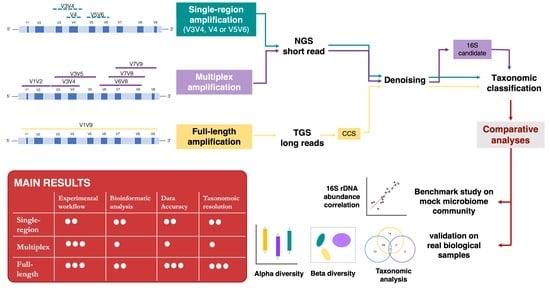
1. Introduction
2. Materials and Methods
2.1. Samples
2.2. 16S rRNA Gene Amplicon-Based Library Preparation and Sequencing
2.3. Bioinformatic Data Analysis
2.3.1. Single-Region Data Analysis
2.3.2. Multiplex Data Analysis
2.3.3. Full-Length Data Analysis
2.3.4. Statistical Analysis
3. Results
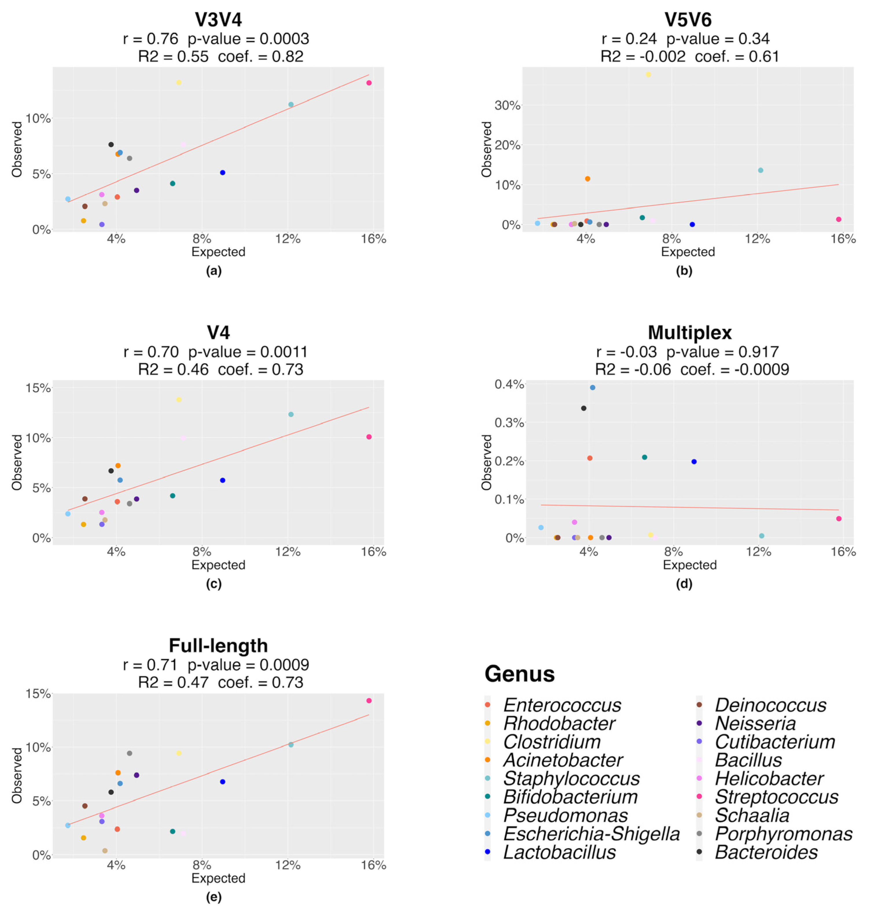
3.1. Mock Benchmark Analysis
3.2. Validation on Real Microbiome Samples
3.2.1. Sequencing Output and Data Processed
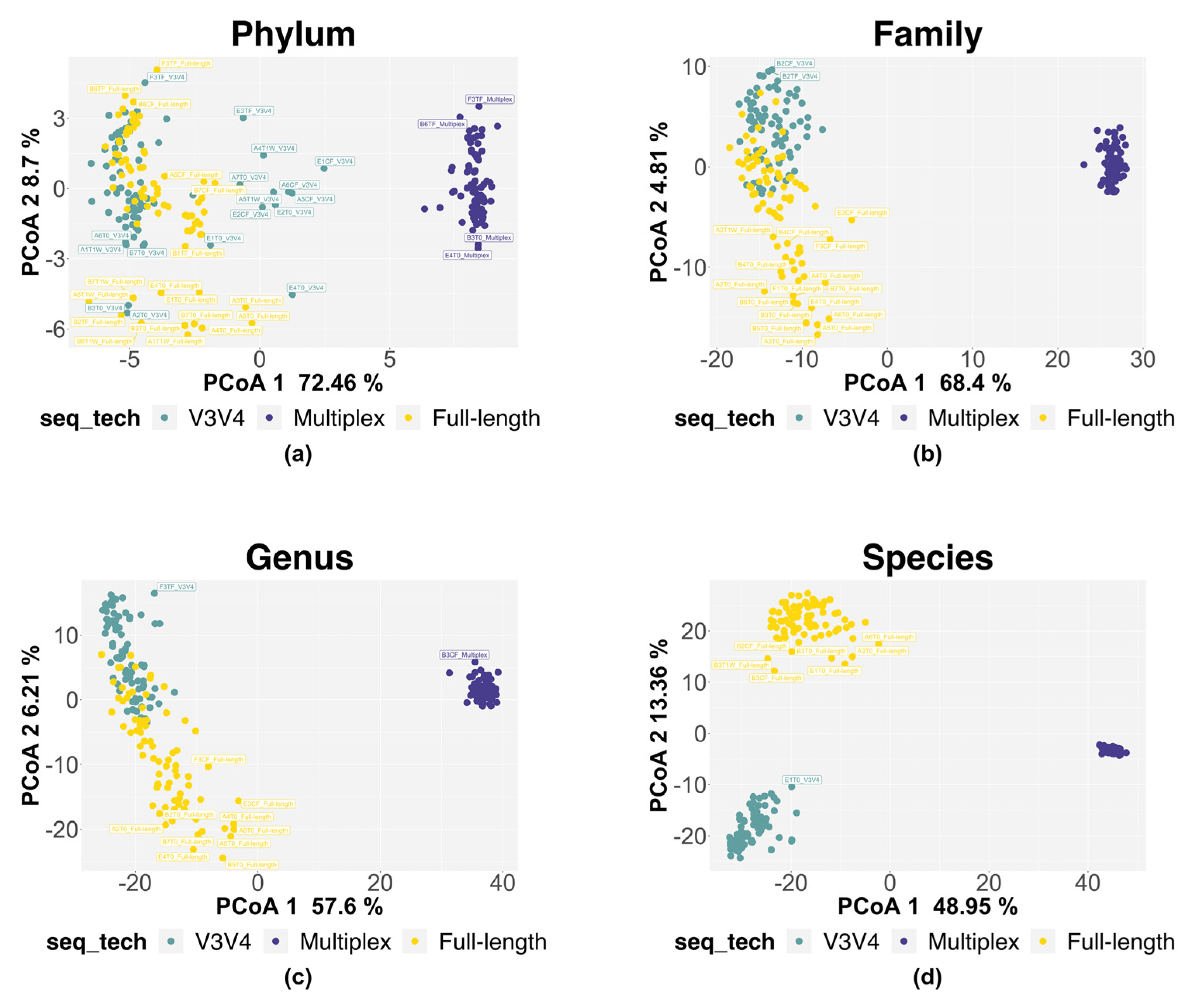
3.2.2. α and β Diversity Analysis
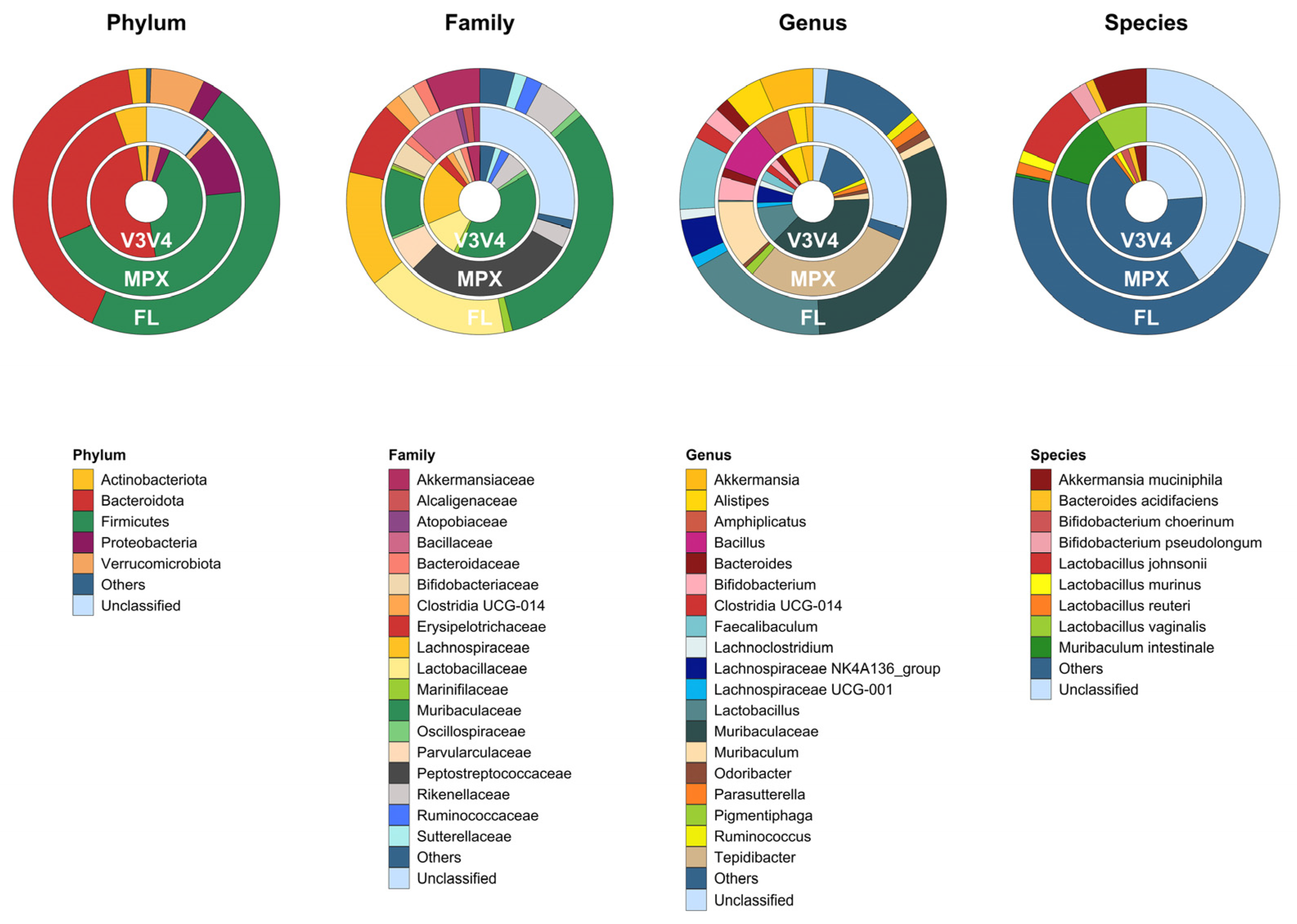
3.2.3. Taxonomic Characterization of the Microbiome
4. Discussion
5. Conclusions
Supplementary Materials
Author Contributions
Funding
Institutional Review Board Statement
Informed Consent Statement
Data Availability Statement
Acknowledgments
Conflicts of Interest
References
- Berg, G.; Rybakova, D.; Fischer, D.; Cernava, T.; Vergès, M.-C.C.; Charles, T.; Chen, X.; Cocolin, L.; Eversole, K.; Corral, G.H.; et al. Microbiome Definition Re-Visited: Old Concepts and New Challenges. Microbiome 2020, 8, 103. [Google Scholar] [CrossRef]
- Malard, F.; Dore, J.; Gaugler, B.; Mohty, M. Introduction to Host Microbiome Symbiosis in Health and Disease. Mucosal. Immunol. 2021, 14, 547–554. [Google Scholar] [CrossRef]
- Durack, J.; Lynch, S.V. The Gut Microbiome: Relationships with Disease and Opportunities for Therapy. J. Exp. Med. 2019, 216, 20–40. [Google Scholar] [CrossRef] [PubMed] [Green Version]
- Thomas, A.M.; Segata, N. Multiple Levels of the Unknown in Microbiome Research. BMC Biol. 2019, 17, 48. [Google Scholar] [CrossRef] [PubMed] [Green Version]
- Pérez-Cobas, A.E.; Gomez-Valero, L.; Buchrieser, C. Metagenomic Approaches in Microbial Ecology: An Update on Whole-Genome and Marker Gene Sequencing Analyses. Microb. Genom. 2020, 6. [Google Scholar] [CrossRef]
- Zhang, L.; Chen, F.; Zeng, Z.; Xu, M.; Sun, F.; Yang, L.; Bi, X.; Lin, Y.; Gao, Y.; Hao, H.; et al. Advances in Metagenomics and Its Application in Environmental Microorganisms. Front. Microbiol. 2021, 12, 766364. [Google Scholar] [CrossRef]
- Amarasinghe, S.L.; Su, S.; Dong, X.; Zappia, L.; Ritchie, M.E.; Gouil, Q. Opportunities and Challenges in Long-Read Sequencing Data Analysis. Genome Biol. 2020, 21, 30. [Google Scholar] [CrossRef] [Green Version]
- Earl, J.P.; Adappa, N.D.; Krol, J.; Bhat, A.S.; Balashov, S.; Ehrlich, R.L.; Palmer, J.N.; Workman, A.D.; Blasetti, M.; Sen, B.; et al. Species-Level Bacterial Community Profiling of the Healthy Sinonasal Microbiome Using Pacific Biosciences Sequencing of Full-Length 16S RRNA Genes. Microbiome 2018, 6, 190. [Google Scholar] [CrossRef] [Green Version]
- Martin, T.C.; Visconti, A.; Spector, T.D.; Falchi, M. Conducting Metagenomic Studies in Microbiology and Clinical Research. Appl. Microbiol. Biotechnol. 2018, 102, 8629–8646. [Google Scholar] [CrossRef] [Green Version]
- Nygaard, A.B.; Tunsjø, H.S.; Meisal, R.; Charnock, C. A Preliminary Study on the Potential of Nanopore MinION and Illumina MiSeq 16S RRNA Gene Sequencing to Characterize Building-Dust Microbiomes. Sci. Rep. 2020, 10, 3209. [Google Scholar] [CrossRef] [Green Version]
- Bharti, R.; Grimm, D.G. Current Challenges and Best-Practice Protocols for Microbiome Analysis. Brief. Bioinform. 2021, 22, 178–193. [Google Scholar] [CrossRef] [PubMed] [Green Version]
- Ficetola, G.F.; Taberlet, P.; Coissac, E. How to Limit False Positives in Environmental DNA and Metabarcoding? Mol. Ecol. Resour. 2016, 16, 604–607. [Google Scholar] [CrossRef] [PubMed] [Green Version]
- Garrido-Sanz, L.; Àngel Senar, M.; Piñol, J. Drastic Reduction of False Positive Species in Samples of Insects by Intersecting the Default Output of Two Popular Metagenomic Classifiers. PLoS ONE 2022, 17, e0275790. [Google Scholar] [CrossRef] [PubMed]
- Bolyen, E.; Rideout, J.R.; Dillon, M.R.; Bokulich, N.A.; Abnet, C.C.; Al-Ghalith, G.A.; Alexander, H.; Alm, E.J.; Arumugam, M.; Asnicar, F.; et al. Reproducible, Interactive, Scalable and Extensible Microbiome Data Science Using QIIME 2. Nat. Biotechnol. 2019, 37, 852–857. [Google Scholar] [CrossRef]
- Wensel, C.R.; Pluznick, J.L.; Salzberg, S.L.; Sears, C.L. Next-Generation Sequencing: Insights to Advance Clinical Investigations of the Microbiome. J. Clin. Investig. 2022, 132, e154944. [Google Scholar] [CrossRef]
- Caporaso, J.G.; Lauber, C.L.; Walters, W.A.; Berg-Lyons, D.; Lozupone, C.A.; Turnbaugh, P.J.; Fierer, N.; Knight, R. Global Patterns of 16S RRNA Diversity at a Depth of Millions of Sequences per Sample. Proc. Natl. Acad. Sci. USA 2011, 108, 4516–4522. [Google Scholar] [CrossRef]
- Liu, X.; Fan, H.; Ding, X.; Hong, Z.; Nei, Y.; Liu, Z.; Li, G.; Guo, H. Analysis of the Gut Microbiota by High-Throughput Sequencing of the V5–V6 Regions of the 16S RRNA Gene in Donkey. Curr. Microbiol. 2014, 68, 657–662. [Google Scholar] [CrossRef]
- Sinclair, L.; Osman, O.A.; Bertilsson, S.; Eiler, A. Microbial Community Composition and Diversity via 16S RRNA Gene Amplicons: Evaluating the Illumina Platform. PLoS ONE 2015, 10, e0116955. [Google Scholar] [CrossRef] [Green Version]
- Hamad, I.; Abou Abdallah, R.; Ravaux, I.; Mokhtari, S.; Tissot-Dupont, H.; Michelle, C.; Stein, A.; Lagier, J.-C.; Raoult, D.; Bittar, F. Metabarcoding Analysis of Eukaryotic Microbiota in the Gut of HIV-Infected Patients. PLoS ONE 2018, 13, e0191913. [Google Scholar] [CrossRef] [Green Version]
- Tsang, C.-C.; Teng, J.L.L.; Lau, S.K.P.; Woo, P.C.Y. Rapid Genomic Diagnosis of Fungal Infections in the Age of Next-Generation Sequencing. J. Fungi 2021, 7, 636. [Google Scholar] [CrossRef]
- Fouhy, F.; Clooney, A.G.; Stanton, C.; Claesson, M.J.; Cotter, P.D. 16S RRNA Gene Sequencing of Mock Microbial Populations- Impact of DNA Extraction Method, Primer Choice and Sequencing Platform. BMC Microbiol. 2016, 16, 123. [Google Scholar] [CrossRef]
- Palkova, L.; Tomova, A.; Repiska, G.; Babinska, K.; Bokor, B.; Mikula, I.; Minarik, G.; Ostatnikova, D.; Soltys, K. Evaluation of 16S RRNA Primer Sets for Characterisation of Microbiota in Paediatric Patients with Autism Spectrum Disorder. Sci. Rep. 2021, 11, 6781. [Google Scholar] [CrossRef] [PubMed]
- Tremblay, J.; Singh, K.; Fern, A.; Kirton, E.S.; He, S.; Woyke, T.; Lee, J.; Chen, F.; Dangl, J.L.; Tringe, S.G. Primer and Platform Effects on 16S RRNA Tag Sequencing. Front. Microbiol. 2015, 6, 771. [Google Scholar] [CrossRef] [PubMed] [Green Version]
- Johnson, J.S.; Spakowicz, D.J.; Hong, B.-Y.; Petersen, L.M.; Demkowicz, P.; Chen, L.; Leopold, S.R.; Hanson, B.M.; Agresta, H.O.; Gerstein, M.; et al. Evaluation of 16S RRNA Gene Sequencing for Species and Strain-Level Microbiome Analysis. Nat. Commun. 2019, 10, 5029. [Google Scholar] [CrossRef] [PubMed] [Green Version]
- Xiao, T.; Zhou, W. The Third Generation Sequencing: The Advanced Approach to Genetic Diseases. Transl. Pediatr. 2020, 9, 163–173. [Google Scholar] [CrossRef] [PubMed]
- Athanasopoulou, K.; Boti, M.A.; Adamopoulos, P.G.; Skourou, P.C.; Scorilas, A. Third-Generation Sequencing: The Spearhead towards the Radical Transformation of Modern Genomics. Life 2021, 12, 30. [Google Scholar] [CrossRef]
- Hoang, M.T.V.; Irinyi, L.; Hu, Y.; Schwessinger, B.; Meyer, W. Long-Reads-Based Metagenomics in Clinical Diagnosis With a Special Focus on Fungal Infections. Front. Microbiol. 2022, 12, 708550. [Google Scholar] [CrossRef]
- Lloyd-Price, J.; Mahurkar, A.; Rahnavard, G.; Crabtree, J.; Orvis, J.; Hall, A.B.; Brady, A.; Creasy, H.H.; McCracken, C.; Giglio, M.G.; et al. Strains, Functions and Dynamics in the Expanded Human Microbiome Project. Nature 2017, 550, 61–66. [Google Scholar] [CrossRef] [Green Version]
- Algieri, F.; Tanaskovic, N.; Rincon, C.C.; Notario, E.; Braga, D.; Pesole, G.; Rusconi, R.; Penna, G.; Rescigno, M. Lactobacillus Paracasei CNCM I-5220-Derived Postbiotic Protects from the Leaky-Gut. Front. Microbiol. 2023, 14, 1157164. [Google Scholar] [CrossRef] [PubMed]
- Marzano, M.; Fosso, B.; Colliva, C.; Notario, E.; Passeri, D.; Intranuovo, M.; Gioiello, A.; Adorini, L.; Pesole, G.; Pellicciari, R.; et al. Farnesoid X Receptor Activation by the Novel Agonist TC-100 (3α, 7α, 11β-Trihydroxy-6α-Ethyl-5β-Cholan-24-Oic Acid) Preserves the Intestinal Barrier Integrity and Promotes Intestinal Microbial Reshaping in a Mouse Model of Obstructed Bile Acid Flow. Biomed. Pharmacother. 2022, 153, 113380. [Google Scholar] [CrossRef]
- The Human Microbiome Project Consortium Structure. Function and Diversity of the Healthy Human Microbiome. Nature 2012, 486, 207–214. [Google Scholar] [CrossRef] [PubMed] [Green Version]
- Piancone, E.; Fosso, B.; Marzano, M.; De Robertis, M.; Notario, E.; Oranger, A.; Manzari, C.; Bruno, S.; Visci, G.; Defazio, G.; et al. Natural and after Colon Washing Fecal Samples: The Two Sides of the Coin for Investigating the Human Gut Microbiome. Sci. Rep. 2022, 12, 17909. [Google Scholar] [CrossRef] [PubMed]
- Manzari, C.; Fosso, B.; Marzano, M.; Annese, A.; Caprioli, R.; D’Erchia, A.M.; Gissi, C.; Intranuovo, M.; Picardi, E.; Santamaria, M.; et al. The Influence of Invasive Jellyfish Blooms on the Aquatic Microbiome in a Coastal Lagoon (Varano, SE Italy) Detected by an Illumina-Based Deep Sequencing Strategy. Biol. Invasions 2015, 17, 923–940. [Google Scholar] [CrossRef] [Green Version]
- Callahan, B.J.; Wong, J.; Heiner, C.; Oh, S.; Theriot, C.M.; Gulati, A.S.; McGill, S.K.; Dougherty, M.K. High-Throughput Amplicon Sequencing of the Full-Length 16S RRNA Gene with Single-Nucleotide Resolution. Nucleic Acids Res. 2019, 47, e103. [Google Scholar] [CrossRef] [Green Version]
- Martin, M. CUTADAPT Removes Adapter Sequences from High-Throughput Sequencing Reads. EMBnet.J. 2011, 17, 10–12. [Google Scholar] [CrossRef]
- Callahan, B.J.; McMurdie, P.J.; Rosen, M.J.; Han, A.W.; Johnson, A.J.A.; Holmes, S.P. DADA2: High-Resolution Sample Inference from Illumina Amplicon Data. Nat. Methods 2016, 13, 581–583. [Google Scholar] [CrossRef] [Green Version]
- Pruesse, E.; Quast, C.; Knittel, K.; Fuchs, B.M.; Ludwig, W.; Peplies, J.; Glockner, F.O. SILVA: A Comprehensive Online Resource for Quality Checked and Aligned Ribosomal RNA Sequence Data Compatible with ARB. Nucleic Acids Res. 2007, 35, 7188–7196. [Google Scholar] [CrossRef] [PubMed] [Green Version]
- Wang, Q.; Garrity, G.M.; Tiedje, J.M.; Cole, J.R. Naïve Bayesian Classifier for Rapid Assignment of RRNA Sequences into the New Bacterial Taxonomy. Appl. Environ. Microbiol. 2007, 73, 5261–5267. [Google Scholar] [CrossRef] [Green Version]
- Edgar, R.C.; Flyvbjerg, H. Error Filtering, Pair Assembly and Error Correction for next-Generation Sequencing Reads. Bioinformatics 2015, 31, 3476–3482. [Google Scholar] [CrossRef] [Green Version]
- Li, H. Minimap2: Pairwise Alignment for Nucleotide Sequences. Bioinformatics 2018, 34, 3094–3100. [Google Scholar] [CrossRef] [Green Version]
- Danecek, P.; Bonfield, J.K.; Liddle, J.; Marshall, J.; Ohan, V.; Pollard, M.O.; Whitwham, A.; Keane, T.; McCarthy, S.A.; Davies, R.M.; et al. Twelve Years of SAMtools and BCFtools. GigaScience 2021, 10, giab008. [Google Scholar] [CrossRef]
- Altschul, S.F.; Gish, W.; Miller, W.; Myers, E.W.; Lipman, D.J. Basic Local Alignment Search Tool. J. Mol. Biol. 1990, 215, 403–410. [Google Scholar] [CrossRef] [PubMed]
- Altschul, S. Gapped BLAST and PSI-BLAST: A New Generation of Protein Database Search Programs. Nucleic Acids Res. 1997, 25, 3389–3402. [Google Scholar] [CrossRef] [PubMed] [Green Version]
- McGinnis, S.; Madden, T.L. BLAST: At the Core of a Powerful and Diverse Set of Sequence Analysis Tools. Nucleic Acids Res. 2004, 32, W20–W25. [Google Scholar] [CrossRef] [PubMed]
- Pedregosa, F.; Varoquaux, G.; Gramfort, A.; Michel, V.; Thirion, B.; Grisel, O.; Blondel, M.; Prettenhofer, P.; Weiss, R.; Dubourg, V.; et al. Scikit-Learn: Machine Learning in Python. J. Mach. Learn. Res. 2012, 12, 2825–2830. [Google Scholar]
- Davis, N.M.; Proctor, D.M.; Holmes, S.P.; Relman, D.A.; Callahan, B.J. Simple Statistical Identification and Removal of Contaminant Sequences in Marker-Gene and Metagenomics Data. Microbiome 2018, 6, 226. [Google Scholar] [CrossRef] [Green Version]
- McMurdie, P.J.; Holmes, S. Phyloseq: An R Package for Reproducible Interactive Analysis and Graphics of Microbiome Census Data. PLoS ONE 2013, 8, e61217. [Google Scholar] [CrossRef] [Green Version]
- Oksanen, J.; Guillaume, F.B.; Roeland, K.; Legendre, P.; Peter, M.; O’Hara, R.B.; Gavin, S.; Peter, S.; Stevenes, M.H.H.; Helene, W. Vegan: Community Ecology Package; R Package Version 2.5-6; The R Project for Statistical Computing: Ames, IA, USA, 2015. [Google Scholar]
- Gloor, G.B.; Macklaim, J.M.; Pawlowsky-Glahn, V.; Egozcue, J.J. Microbiome Datasets Are Compositional: And This Is Not Optional. Front. Microbiol. 2017, 8, 2224. [Google Scholar] [CrossRef] [Green Version]
- Lin, H.; Peddada, S.D. Analysis of Compositions of Microbiomes with Bias Correction. Nat. Commun. 2020, 11, 3514. [Google Scholar] [CrossRef]
- Nejman, D.; Livyatan, I.; Fuks, G.; Gavert, N.; Zwang, Y.; Geller, L.T.; Rotter-Maskowitz, A.; Weiser, R.; Mallel, G.; Gigi, E.; et al. The Human Tumor Microbiome Is Composed of Tumor Type–Specific Intracellular Bacteria. Science 2020, 368, 973–980. [Google Scholar] [CrossRef]
- Ciuffreda, L.; Rodríguez-Pérez, H.; Flores, C. Nanopore Sequencing and Its Application to the Study of Microbial Communities. Comput. Struct. Biotechnol. J. 2021, 19, 1497–1511. [Google Scholar] [CrossRef] [PubMed]
- Portik, D.M.; Brown, C.T.; Pierce-Ward, N.T. Evaluation of Taxonomic Classification and Profiling Methods for Long-Read Shotgun Metagenomic Sequencing Datasets. BMC Bioinform. 2022, 23, 541. [Google Scholar] [CrossRef] [PubMed]
- Tourlousse, D.M.; Narita, K.; Miura, T.; Ohashi, A.; Matsuda, M.; Ohyama, Y.; Shimamura, M.; Furukawa, M.; Kasahara, K.; Kameyama, K.; et al. Characterization and Demonstration of Mock Communities as Control Reagents for Accurate Human Microbiome Community Measurements. Microbiol. Spectr. 2022, 10, e01915-21. [Google Scholar] [CrossRef] [PubMed]
- Liu, P.-Y.; Wu, W.-K.; Chen, C.-C.; Panyod, S.; Sheen, L.-Y.; Wu, M.-S. Evaluation of Compatibility of 16S RRNA V3V4 and V4 Amplicon Libraries for Clinical Microbiome Profiling. BioRxiv 2020. [Google Scholar] [CrossRef]
- Hsieh, Y.-P.; Hung, Y.-M.; Tsai, M.-H.; Lai, L.-C.; Chuang, E.Y. 16S-ITGDB: An Integrated Database for Improving Species Classification of Prokaryotic 16S Ribosomal RNA Sequences. Front. Bioinform. 2022, 2, 905489. [Google Scholar] [CrossRef]
- Quast, C.; Pruesse, E.; Yilmaz, P.; Gerken, J.; Schweer, T.; Yarza, P.; Peplies, J.; Glöckner, F.O. The SILVA Ribosomal RNA Gene Database Project: Improved Data Processing and Web-Based Tools. Nucleic Acids Res. 2012, 41, D590–D596. [Google Scholar] [CrossRef] [PubMed]
- Maidak, B.L.; Cole, J.R.; Parker, C.T.; Garrity, G.M.; Larsen, N.; Li, B.; Lilburn, T.G.; McCaughey, M.J.; Olsen, G.J.; Overbeek, R.; et al. A New Version of the RDP (Ribosomal Database Project). Nucleic Acids Res. 1999, 27, 171–173. [Google Scholar] [CrossRef] [PubMed] [Green Version]
- DeSantis, T.Z.; Hugenholtz, P.; Larsen, N.; Rojas, M.; Brodie, E.L.; Keller, K.; Huber, T.; Dalevi, D.; Hu, P.; Andersen, G.L. Greengenes, a Chimera-Checked 16S RRNA Gene Database and Workbench Compatible with ARB. Appl. Environ. Microbiol. 2006, 72, 5069–5072. [Google Scholar] [CrossRef] [Green Version]
- Hiergeist, A.; Ruelle, J.; Emler, S.; Gessner, A. Reliability of Species Detection in 16S Microbiome Analysis: Comparison of Five Widely Used Pipelines and Recommendations for a More Standardized Approach. PLoS ONE 2023, 18, e0280870. [Google Scholar] [CrossRef]
- Finotello, F.; Trajanoski, Z. Quantifying Tumor-Infiltrating Immune Cells from Transcriptomics Data. Cancer Immunol. Immunother. 2018, 67, 1031–1040. [Google Scholar] [CrossRef]
- Hou, K.; Wu, Z.-X.; Chen, X.-Y.; Wang, J.-Q.; Zhang, D.; Xiao, C.; Zhu, D.; Koya, J.B.; Wei, L.; Li, J.; et al. Microbiota in Health and Diseases. Sig. Transduct. Target Ther. 2022, 7, 135. [Google Scholar] [CrossRef] [PubMed]


| Expected Genera | Observed Genera | ||||
|---|---|---|---|---|---|
| V3V4 | V5V6 | V4 | Multiplex | Full-Length | |
| Enterococcus | |||||
| Rhodobacter | |||||
| Clostridium § | |||||
| Acinetobacter | |||||
| Staphylococcus | |||||
| Bifidobacterium | |||||
| Pseudomonas | |||||
| Escherichia-Shigella | |||||
| Lactobacillus | |||||
| Deinococcus | |||||
| Neisseria | |||||
| Cutibacterium | |||||
| Bacillus | |||||
| Helicobacter | |||||
| Streptococcus | |||||
| Schaalia §§ | |||||
| Porphyromonas | |||||
| Bacteroides | |||||
| Total observed/expected | 18/18 | 10/18 | 18/18 | 10/18 | 18/18 |
| Expected Species | Observed Species | ||||
|---|---|---|---|---|---|
| V3V4 | V5V6 | V4 | Multiplex | Full-Length | |
| Acinetobacter baumannii | |||||
| Bacillus pacificus | |||||
| Bacteroides vulgatus | |||||
| Bifidobacterium adolescentis | |||||
| Clostridium beijerinckii | |||||
| Cutibacterium acnes | |||||
| Deinococcus radiodurans | |||||
| Enterococcus faecalis | |||||
| Escherichia coli | |||||
| Helicobacter pylori | |||||
| Lactobacillus gasseri | |||||
| Neisseria meningitidis | |||||
| Porphyromonas gingivalis | |||||
| Pseudomonas aeruginosa | |||||
| Rhodobacter sphaeroides | |||||
| Schaalia odontolytica | |||||
| Staphylococcus aureus | |||||
| Staphylococcus epidermidis | |||||
| Streptococcus agalactiae | |||||
| Streptococcus mutans | |||||
| Total observed | 12/20 | 4/20 | 9/20 | 4/20 | 15/20 |
| Genus | Species | |||||
|---|---|---|---|---|---|---|
| Precision (%) | Accuracy (%) | Recall (%) | Precision (%) | Accuracy (%) | Recall (%) | |
| V3V4 | 77.11 | 77.14 | 100 | 99.71 | 54.93 | 54.77 |
| V5V6 | 33.63 | 29.84 | 71.16 | 1.49 | 1.49 | 4.20 |
| V4 | 78.39 | 78.42 | 100 | 99.44 | 33.20 | 33.10 |
| Multiplex | 11.16 | 74.13 | 1.20 | 2.96 | 73.91 | 0.32 |
| Full-length | 83.50 | 83.50 | 100 | 99.95 | 78.10 | 78.11 |
| V3V4 | Multiplex | Full-Length | |
|---|---|---|---|
| Sequencing Platform | Illumina MiSeq | Illumina MiSeq | PacBio Sequel II System |
| Final Output (n° reads) | 28,200,000 | 13,520,000 | 2,529,947 |
| Mean read number/sample | 180,769 ± 39,538 | 146,153 ± 57,231 | 28,263 ± 12,487 |
| Mean reads length (bp) | 275 | 250 | 1500 |
| Phylum-Level Data | Family-Level Data | Genus-Level Data | Species-Level Data | |||||
|---|---|---|---|---|---|---|---|---|
| Pairwise Comparison | R2 (%) | p-Value | R2 (%) | p-Value | R2 (%) | p-Value | R2 (%) | p-Value |
| V3V4 vs. FL | 12.20 | <0.001 | 11.80 | <0.001 | 12.54 | <0.001 | 27.65 | <0.001 |
| Residuals | 87.80 | 88.20 | 87.46 | 72.35 | ||||
| V3V4 vs. MPX | 78.18 | <0.001 | 78.23 | <0.001 | 71.49 | <0.001 | 71.35 | <0.001 |
| Residuals | 21.82 | 21.77 | 28.51 | 28.65 | ||||
| MPX vs. FL | 74.80 | <0.001 | 71.47 | <0.001 | 60.63 | <0.001 | 59.64 | <0.001 |
| Residuals | 25.20 | 28.53 | 39.37 | 40.36 | ||||
Disclaimer/Publisher’s Note: The statements, opinions and data contained in all publications are solely those of the individual author(s) and contributor(s) and not of MDPI and/or the editor(s). MDPI and/or the editor(s) disclaim responsibility for any injury to people or property resulting from any ideas, methods, instructions or products referred to in the content. |
© 2023 by the authors. Licensee MDPI, Basel, Switzerland. This article is an open access article distributed under the terms and conditions of the Creative Commons Attribution (CC BY) license (https://creativecommons.org/licenses/by/4.0/).
Share and Cite
Notario, E.; Visci, G.; Fosso, B.; Gissi, C.; Tanaskovic, N.; Rescigno, M.; Marzano, M.; Pesole, G. Amplicon-Based Microbiome Profiling: From Second- to Third-Generation Sequencing for Higher Taxonomic Resolution. Genes 2023, 14, 1567. https://doi.org/10.3390/genes14081567
Notario E, Visci G, Fosso B, Gissi C, Tanaskovic N, Rescigno M, Marzano M, Pesole G. Amplicon-Based Microbiome Profiling: From Second- to Third-Generation Sequencing for Higher Taxonomic Resolution. Genes. 2023; 14(8):1567. https://doi.org/10.3390/genes14081567
Chicago/Turabian StyleNotario, Elisabetta, Grazia Visci, Bruno Fosso, Carmela Gissi, Nina Tanaskovic, Maria Rescigno, Marinella Marzano, and Graziano Pesole. 2023. "Amplicon-Based Microbiome Profiling: From Second- to Third-Generation Sequencing for Higher Taxonomic Resolution" Genes 14, no. 8: 1567. https://doi.org/10.3390/genes14081567